Determining the distribution of probes between different subcellular locations through automated unmixing of subcellular patterns

Abstract

Many proteins or other biological macromolecules are localized to more than one subcellular structure. The fraction of a protein in different cellular compartments is often measured by colocalization with organelle-specific fluorescent markers, requiring availability of fluorescent probes for each compartment and acquisition of images for each in conjunction with the macromolecule of interest. Alternatively, tailored algorithms allow finding particular regions in images and quantifying the amount of fluorescence they contain. Unfortunately, this approach requires extensive hand-tuning of algorithms and is often cell type-dependent. Here we describe a machine-learning approach for estimating the amount of fluorescent signal in different subcellular compartments without hand tuning, requiring only the acquisition of separate training images of markers for each compartment. In testing on images of cells stained with mixtures of probes for different organelles, we achieved a 93% correlation between estimated and expected amounts of probes in each compartment. We also demonstrated that the method can be used to quantify drug-dependent protein translocations. The method enables automated and unbiased determination of the distributions of protein across cellular compartments, and will significantly improve imaging-based high-throughput assays and facilitate proteome-scale localization efforts.

Eukaryotic cells are organized into a number of distinct subcellular compartments and structures that play critical roles in cellular functions. Therefore, protein localization is a tightly regulated process whose failure may lead to severe pathologies (1). Nuclear translocation is well-known example of a regulated subcellular compartmentalization event, and it has been the subject of many studies uncovering its association to human pathologies, such as cancer (1 –4). Because the nucleus is a large and easily distinguishable structure, such translocation can readily be measured in an automated fashion. Unfortunately, detecting and quantifying the amount of macromolecules in smaller organelles are much harder tasks to perform using traditional techniques, and they are not readily automated. The problem is made more difficult by the fact that proteins (and other macromolecules) are often found in more than one subcellular structure.

The traditional approach to determining the amount of a macromolecule in specific compartments is measuring colocalization of that molecule with organelle-specific markers labeled with a different fluorophore. This approach is often used for one or a few proteins whose possible locations are known a priori, and recent work has described methods for automatically measuring the fraction of colocalization (5, 6); however, it is difficult to apply on a proteome-wide basis because it requires the availability of probes for all possible compartments and the collection of separate images of each protein in combination with each marker. An exciting automated approach that builds on the basic colocalization method is the MELK technology, which uses robotics to carry out successive rounds of staining for different macromolecules on a given cell sample or tissue (7). However, this approach is restricted to fixed samples and cannot be used for analysis of dynamic pattern changes in living cells. Hand-tuned algorithms for distinguishing particular subcellular regions are also widely used as an alternative to colocalization in high-content screening (8), but they typically are only able to distinguish major cellular regions and are not easily transferred to the analysis of other regions or cell types.

Beginning with the demonstration that automated recognition of subcellular patterns was feasible (9, 10), our group and others have created systems that are able to classify all major subcellular location patterns, and to do so with a higher accuracy than visual analysis (11 –14). Automated systems can also learn what subcellular patterns are present in large collections of images without prior knowledge of the possible patterns (13, 15). However, such pattern-clustering approaches have two major limitations. First, they treat each unique combination of major, fundamental patterns as a new pattern because they cannot readily identify the fundamental patterns of which it is composed. Second, they are not designed to handle cases where the fraction of mixing between two patterns can vary continuously, because such continua are either considered as one large pattern or arbitrarily divided into subpatterns.

Thus, we sought to develop tools to quantify the amount of fluorescence in each compartment for images containing a mixture of fundamental patterns, assuming that sets of images containing each fundamental pattern are available. We have previously proposed an object-based approach (16) to this problem that consisted of two learning stages: learning what object types are present in the fundamental patterns, and learning how much fluorescence is present in each object type in each pattern. The fraction of fluorescence in each fundamental pattern for a mixed image was then estimated by determining the mixture coefficients that were most likely to have given rise to that image. This method was tested on synthetic images created from known amounts of many patterns, which permitted the accuracy of unmixing of a given image to be determined by comparison with the mixture coefficients used to synthesize it. However, the effectiveness of this approach on real images with multiple patterns was not determined because of the lack of availability of real images for which mixture fractions were known. In this study, we used high-throughput automated microscopy to create an image dataset for cells labeled with varying mixtures of fluorescent mitochondrial and lysosomal probes containing essentially the same fluorophore. This controlled experiment mimics typical cases, such as a protein that distributes among different organelles or that changes its location upon drug stimulation. Therefore, these data offer the perfect conditions to test our algorithm in the context of automated image acquisition. We were able to unmix the two different patterns and quantify the relative amount of probes in the two organelles. We were also able to show that the method can identify objects and patterns that are distinct from those used for training. This work should therefore open the door to a more comprehensive approach to subcellular pattern analysis for automated microscopy. In part, the strategy described here should help quantify subtle translocation and localization defects that could not be readily measured previously. To assess the usefulness of this methodology in automated screening, we applied our algorithms to quantify autophagocytosis by monitoring the distribution of microtubule associated protein light chain 3 (LC3) into autophagosomes upon Bafilomycin A1 (BAF) treatment.

Results

In this article, a “pattern” designates the subcellular distribution of a protein, or of a set of proteins whose distributions are statistically indistinguishable. We define a “fundamental pattern” as a pattern that cannot be represented as the sum of the patterns of other proteins, while a “mixed pattern” refers to a distribution consisting of two or more fundamental patterns. A pattern is characterized by a collection of fluorescent objects whose shape, size, and intensity vary within cells. For example, nuclei are typically large ellipsoidal objects, while lysosomes are small and generally have spherical shapes. The method we describe here seeks to estimate the components in a given mixed image based on two assumptions. The first is that the set of discrete object types resulting from segmentation of images containing a mixed pattern is essentially the same as the union of the sets of object types found in images of each of its fundamental patterns (i.e., that any new object types that might be found only in mixed images do not contain a significant amount of fluorescence and can be safely ignored). The second is that the amount of fluorescence in each object type in a mixed image is approximately the sum over all fundamental patterns of the product of the fraction of total protein in that pattern and the number of objects of that type in images of that pattern (i.e., that any differences between the actual and expected sums are sufficiently small and uncorrelated with the mixture fractions that they do not systematically affect estimates of the fractions). The approach is illustrated in Fig. 1 for mixtures of two patterns, but it generalizes to any number of patterns. The details for each step of this process are described in Materials and Methods. We assume that we are provided with a collection of images of cells containing varying combinations of fluorescent probes, such as for the multiwell plate of pure and mixed samples depicted in Fig. 1A. The two probes are assumed to be imaged using filters that do not distinguish between the probes. Wells containing pure probes are symbolically represented along the outer row and column (with example images shown in Fig. 1 B and C), and the other locations represent mixed conditions (a mixed image is shown in Fig. 1D). The starting point for unmixing is finding all objects in each image by thresholding (Fig. 1E). Each object is described using a set of numerical features that measure characteristics such as size and shape. The two sets of fundamental patterns (pure probes) are used to learn the types of objects that can be found (Fig. 1F). Given this list of object types, the distribution of object types across each fundamental pattern is then learned as a count of the number of objects in each object type (Fig. 1G). Given this, the distribution of fluorescence in each object type in a mixed image (Fig. 1H) can be used to estimate the fraction of probe in each fundamental type.

Fig. 1.

Subcellular pattern unmixing approach. (A) The starting point is a collection of images (typically from a multiwell plate) in which various concentrations of two probes are present (the concentrations of the Mitotracker and Lysotracker probes are shown by increasing intensity of red and green, respectively). Example images are shown for wells containing just Mitotracker (B), just Lysotracker (C), or a mixture of the two probes (D). The steps in the analysis process are shown: finding objects (E), learning object types (illustrated schematically as objects with different sizes and shapes) (F), learning the object type distributions for the two fundamental patterns (G), and unmixing a mixed object type distribution (H).

In prior work, we demonstrated that this approach could give reasonable estimates of mixture fractions for images synthesized by combining objects from images of pure patterns (average accuracies of around 80% were obtained) (16). These synthetic tests were carried out using a collection of high-resolution images of HeLa cells (11), but left open the question of whether this approach could be used for real images containing mixed patterns.

To address this question, a dataset of mixed patterns is needed in which the mixture fractions are known (at least approximately), so that estimates obtained by unmixing can be compared with expectation. We have therefore constructed such a dataset using high-throughput microscopy. We chose two fluorescent probes (Lysotracker green and Mitotracker green) that stain distinct subcellular compartments (lysosomes and mitochondria) but that contain similar fluorophores, so that they can be imaged together. The dataset contains images for cells incubated with each probe separately (at different concentrations) as well as images for cells incubated with mixtures of the probes. We refer to the single probe images as “training images,” and the mixed images as “testing images.” We assume that the amount of probe fluorescence in each compartment is proportional to the concentration of that probe added. This represents a good simulation of the images expected for a protein that can be found in varying amounts between two compartments.

Object Extraction and Feature Calculation.

As outlined above, the starting point is to identify each fluorescence-containing object in all images. We use an automatically chosen global threshold for each image, as this approach does not require segmentation of the image into individual cell regions. Each object is then described by a set of 11 features that characterize its size, shape, and distance from the nearest nucleus (see Materials and Methods). If more than one image (field) is available for a given condition, the objects from all fields are combined.

Object-Type Learning.

Having identified the individual objects, we next determine how many types of objects are present. We define an object type as a group of objects with similar characteristics. Rather than specifying the object types a priori, we used cluster analysis to learn clusters from the set of all of objects in all of the training images. Although many different clustering methods might be used for this step, we have used k-means clustering because of the large number of objects in the training set. The optimal number of clusters k was determined by minimizing the Akaike Information Criterion, which specifies a tradeoff between complexity of the model (number of clusters) and its goodness (compactness of the clusters). As shown in Fig. S1, this value declines with increasing k until reaching a minimum at a k value of 11.

Learning the Object Composition of Fundamental Patterns.

Once k is known, each fundamental pattern p can be represented as a vector of length k consisting of the frequency of each object type. As shown in Fig. 2, the frequency of each object type is quite different between the lysosomal and mitochondrial patterns.

Fig. 2.

Distribution of object types within fundamental patterns. The average number of objects of each type is shown for the combination of all images of U2OS cells stained with either Mitotracker (black) or Lysotracker (white). The object types are sorted according to the difference between the numbers of objects in the two patterns. Thus, the lowest numbered object types are primarily found in Mitotracker-stained cells, while the highest numbered object types are primarily found in Lysotracker-stained cells. The model power is 0.448 when trained with object frequency distributions and 0.654 when trained with fluorescence fraction distributions.

Estimating Unmixing Fractions.

The type of each object in the training images is known (because all objects in the training images were used for clustering); however, the type of objects in the testing images is not. Each protein object in a testing image was therefore assigned to the cluster whose center was closest to it in the feature space. The frequency and the total fluorescence of all objects belonging to the same type were calculated for each test image.

The average fraction of mitochondrial and lysosomal patterns in each well was then estimated by three different approaches using both the object types and object features (see Materials and Methods). Two of these methods use the number of objects of each type to estimate mixing fractions. The third uses the amount of fluorescence in each type, which depends on the assumption that this amount is linearly dependent upon the concentration of each probe (Fig. S2).

The results for the three methods are compared with those expected from the relative probe concentrations in Fig. 3. The correlation coefficients between estimated and expected fractions are 0.73, 0.77, and 0.83. An example of the correlation between estimated and actual concentrations is shown in Fig. S3. Analysis of the effect of removing nondiscriminative object types is shown in Fig. S4.

Fig. 3.

Expected and estimated pattern fraction for three unmixing methods for the U2OS dataset. The balance between lysosomal and mitochondrial pattern (either expected or estimated) is represented as the fraction of the total pattern (black, 100% mitochondrial; white, 100% lysosomal). For the expected fraction, this is estimated as linearly proportional to the ratio of the relative concentration of the mitochondrial probe to the sum of the relative concentration of the lysosomal and mitochondrial probes (where relative concentration is defined as fraction of the maximum subsaturating concentration).

Removing Outliers.

The unmixing method can be applied without any restrictions to any test images. However, if the mixed patterns in test images contain additional fundamental patterns not present in the training sets, the estimates of mixing fractions will be incorrect. Our solution consists of two steps. The first step is to exclude objects in test images that do not appear to belong to any of the object types found in the training images (outlier objects). The second step is to flag as outlier patterns those test images that during unmixing have large fitting error (i.e., rejecting images that cannot be successfully decomposed into the specified fundamental patterns). Because we cannot know a priori what kinds of new objects might be encountered, both steps use hypothesis-based tests to find thresholds that retain high accuracy for unmixing the training patterns. To test this approach, we used images in which either the nucleus or the endoplasmic reticulum (ER) was marked. Our results show that this methodology can completely remove nuclear objects during the first level outlier detection (Fig. 4A). For the more difficult case of ER staining, the second level detection recognizes most of the ER-containing images as outlier patterns but retains high accuracy of fundamental pattern unmixing (Fig. 4B).

Fig. 4.

Effectiveness of outlier removal methods. (A) Nuclear images were used as outliers. Unmixing accuracies for both inliers (squares, mitochondrial and lysosomal objects) and outlier objects (triangles) with first-level outlier exclusion were approximated by cross validation under different chosen accuracy levels for the U2OS dataset. Nuclear fluorescence was totally removed at all accuracy levels. (B) ER pattern images were used as outliers. Average outlier recognition testing-accuracies for both inliers (squares, mitochondrial and lysosomal images) and outlier images (triangles) with second-level outlier exclusion were approximated by cross validation under different chosen accuracy levels for the BEAS2B dataset. The best separation is obtained using a 75–80% inlier confidence level.

Application Example: Unmixing Drug-Treated Cell Images.

To further test the usefulness of our unmixing algorithms, we tested whether these tools could correctly estimate the accumulation of the microtubule associated protein LC3 into autophagosomes upon BAF treatment. BAF, an inhibitor of the vacuolar ATPase (17, 18), can inhibit autophagy and promotes autophagosome accumulation by preventing vesicular acidification (19). In this experiment, an RT112 cell line stably expressing eGFP-LC3 was treated with various amounts of BAF for 4 h before being fixed and imaged.

To establish the fundamental patterns, the model was trained on images of cells treated with the maximum concentration of drug and of cells that did not undergo any treatment. Unmixing using different methods resulted in a sigmoid-like transition between the two patterns as a function of the drug concentration (Fig. 5). This example illustrates how our unmixing analysis can be applied to provide a quantitative analysis of protein dynamics.

Fig. 5.

Application of pattern unmixing to drug effects. Cells were treated with various concentrations of Bafilomycin a1 (BAF) and images from samples receiving the highest dose and images from untreated cells were used to train an unmixing model. The fraction of drug treated pattern as a function of concentration of drug was estimated using linear unmixing (squares), multinomial unmixing (circles), and fluorescence fraction unmixing (triangles). eGFP-LC3 showed a gradual relocation between the two patterns as a function of BAF concentration.

Discussion

Our group has previously described approaches to cluster proteins based on their subcellular distribution (13, 15). A logical extension of this work is to create tools to estimate the distribution of fluorescently labeled macromolecules between distinct compartments, and we have previously demonstrated such approaches provide good results for synthetic images (16). Here we show that this approach works well on real images obtained from mixed patterns and is suitable for high-throughput microscopy, technology that would arguably benefit the most from such a strategy. Our test mimicked the case of a tagged protein whose distribution varies between two organelles. Because we controlled the amount of both dyes applied to a given cell sample, it was easy to verify whether or not our predictions about the proportion of mitochondrial or lysosomal labeling were accurate. The successful results described here validate the effectiveness of the two-stage, object-based unmixing method on real image data. They also validate our assumption that new object types that might arise do not drastically inhibit unmixing accuracy.

The tool we have described requires only a set of images for each of the pure patterns (for varying levels of expression, if desired) and a set of images for mixed patterns acquired under the same conditions. Incorporation of outlier tests and accuracy estimates makes the approach robust to unanticipated phenotypes. It is also important to note that the fluorophores used for training and testing need not correspond. For example, a system trained on GTP-tagged proteins could be used to unmix an image of an RFP-tagged protein (assuming that the tags do not alter the protein localization). However, because most cell types show different morphologies, it is unlikely that a system trained for one type could be applicable to others.

The success of the experiments described here should provide the capacity to better describe what may be complex effects of drugs or disease on protein location. The tool offers a previously unexplored method to determine a precise and objective subcellular distribution of gene products for various physiological contexts and genetic backgrounds. This approach can also aid large-scale projects, such as proteome-wide localization studies, because it has been tested for images acquired using automated microscopy.

Materials and Methods

Tissue Culture.

U20S cells were grown in D-MEM (Invitrogen), containing 10% FBS (HyClone). The BEAS2B cell line was grown in a F12/D-MEM[1:1] (Invitrogen) containing 10% FBS (HyClone). All media were supplemented with 100 μg/mL of Penicillin-streptomycin and L-Glutamine. A total of 7,000 cells per well were plated in 384-well plates in Phenol-red free Optimem (Gibco) containing 2% serum. After 24 h, Phenol red-free Optimem containing various concentrations (see Fig. 1) of either Mitotracker green or Lysotracker green (Molecular Probes), as well as 2.5 μg/mL Hoechst 33342 (Molecular Probes), was added. In some cases, ERtracker green (Molecular Probes) was added to test the outlier removal algorithm. A total of six replicas of an 8 × 8 matrix of various concentrations of Mitotracker and Lysotracker were dispensed in each plate. After a 30-min incubation, the living cells were imaged by high throughput microscopy.

For experiments analyzing drug effects, RT112 cells were plated in a 1,536-well plate at 500 cells per well and grown for 24 h before being treated with various amounts of BAF. After 4 h, cells were fixed with 1× Mirskys fixative and stained with Hoechst as above.

High-Content Imaging.

Images were acquired using an Opera automated microscope equipped with Nipkow confocal spinning disks (Perkin-Elmer). Cells were kept viable by a built-in incubation chamber. The Hoechst stain, which marks the nuclei, was detected using 405-nm laser excitation and a 450/50-nm emission filter, while Mitotracker, Lysotracker, ERtracker, and eGFP (enhanced GFP) were detected with 488-nm laser excitation and a 535/50 emission filter. To minimize fluorescence cross-talk, the two channels were collected sequentially. To provide a sufficient spatial resolution for the analysis, images were collected using a 40×, 0.9 NA water immersion objective. For each well of the 384-well plate, 35 adjacent fields with 1.5% overlap organized in a 7 × 5 rectangle were collected. Each field usually contained about 20 cells; a small number of out-of-focus images in some wells were automatically discarded.

Image Analysis.

Preprocessing.

Images containing no nuclei and out-of-focus images were removed by thresholding on total Hoechst fluorescence. Shading and skew corrections were performed on remaining images to compensate for nonhomogeneous illumination and differences in registration between channels. Background fluorescence was removed by subtracting the most common pixel value from each pixel.

Object detection.

An automated threshold method (20) was used to distinguish probe-containing from nonprobe-containing pixels. In the resulting binary images, each set of connected above-threshold pixels (an object) was identified. Objects containing fewer than 5 pixels were ignored. The same approach was applied on the DNA channel to identify DNA objects.

Object feature calculation.

To describe the properties of each object, a set of subcellular object features, SOF1, was calculated as described previously (16). This set is composed of nine features based on morphological properties of the object and two features describing the spatial relationship between objects and the cell nucleus. However, because in the experiments described here images were not segmented into single cells, feature SOF1.2 was replaced by the average distance between each object and the nearest nucleus. All features were normalized to zero mean and unit standard deviation calculated using the training data (Z-scores).

Object-type learning.

The features for all objects from the singly-stained samples were clustered using the NetLab k-means function. The quality of the clustering was assessed using the Akaike Information Criterion as described previously (16). For test images, objects were assigned to the cluster whose center was the smallest Euclidean distance from it.

Linear unmixing.

Once the k-object types are defined, each image can be represented as a vector of the frequency of each object type in that image. We define u as the total number of fundamental patterns. For u = 2, a mixture of pattern 1 (lysosomal) with n₁ objects of a specific object type and pattern 2 (mitochondrial) with n₂ objects of the same object type is assumed to generate a mixed pattern with n₁+ n₂ objects of this type.

We assume that mixed pattern object frequencies are linear combinations of fundamental pattern object frequencies as follows:

where α_p represents the proportion of fundamental pattern p in the composition of the mixture. Therefore, a mixed pattern can be represented by a vector of coefficients , containing the fraction of fundamental patterns of which it is composed. Unmixing the mixture pattern consists of solving the linear equation above. Because we have k equations for all object types and only two fundamental patterns (u = 2), a reasonable solution is to minimize the squared error under constraint . Because the contribution of any fundamental pattern cannot be negative, nonnegative constraints are included. The solution was found using quadratic programming methods (the Matlab lsqlin function).

Multinomial unmixing.

An alternative method for unmixing is based on the fact that the number of objects of each type varies between cells even within the same pattern (e.g., the number of small lysosomes can vary from cell to cell). We can reasonably assume that if we learn the distribution of the number of objects per cell of a given type for a given fundamental pattern that it will also apply to the distribution of that object type in a mixed sample. In a multinomial distribution, each object belongs in exactly one of the k possible object types with the probabilities (so that and ). Therefore, each fundamental pattern is represented by a multinomial distribution where is the probability that an object from pattern p belongs to the object type i. This can be estimated by the maximum likelihood estimator of a multinomial distribution:

where corresponds to the number of objects of pattern p which are of type i. Mixed patterns are represented by a multinomial distribution composed of a linear combination of fundamental pattern distribution parameters,

To reach a distribution which best fits the data of mixed pattern conditions, we adjust the coefficients to maximize the likelihood of the object frequency for all k types:

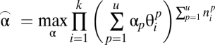An equivalent problem would be to maximize the log likelihood. We have previously deduced closed forms of the first-order derivative and the Hessian matrix, and proved concaveness of the log likelihood function (16). Therefore, Newton’s method was adopted to solve the optimization problem.

Fluorescence fraction unmixing.

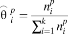
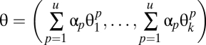
In addition to using the number of objects of each object type to estimate pattern fractions, we can also use the amount of fluorescence in each object type. To do this, we first find the average fraction of fluorescence within each object type i for each fundamental pattern p. We also determine a constant L_k for each probe that relates the concentration of that probe to the expected amount of total fluorescence in all objects of the pattern k labeled by that probe. We combine these to calculate as the amount of fluorescence within each object type that is expected per unit of probe added (assuming that fluorescence is roughly linear over the range of probe concentrations added). The fluorescence expected in each object type is then given by

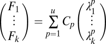where C_p is the concentration of probe that labels pattern p. We used the pseudoinverse approach to estimate this amount.

Outlier detection.

To address the possibility that a particular pattern being unmixed is not a mixture of the fundamental patterns used during training (that is, that it might contain other patterns as well), we developed a two-level outlier detection method. The unmixing results were expressed as , where is the fluorescent fraction of any unrecognized pattern (outliers) and _u is the total number of fundamental patterns. Both levels use statistical hypothesis tests to determine outliers. First, we used a χ² test to remove outlier objects that were not similar to any of the object types learned from the fundamental pattern images. The χ² statistic is defined as , where is the feature of an object and m is the total number of features. Statistics of test object were tested under every χ² distribution learned from each object type in the training images to see if it was from that distribution. An object was considered an outlier if it was rejected by all tests at a specified confidence level . Because a proper value for is hard to determine a priori, we chose it by a linear search using unmixing of the fundamental patterns. The fundamental pattern images were split into training and test sets and the accuracy was reported as the fraction of objects that were associated with the correct pattern. For various , we used cross validation to get averaged accuracies. Accuracy improves with decreasing cut-offs, in other words, with a stricter criterion, more objects are excluded as outliers. We chose an arbitrary acceptable accuracy level and its associated level to remove outlier objects in testing images.

Similarly, we performed a hypothesis test to exclude mixed patterns that had large fitting errors when decomposed into fractional combination of fundamental pattern fluorescence fractions. This fitting error statistics was defined as:

Statistics of a test-pattern fluorescence fraction was compared with the empirical distribution of the fitting error. Pattern was rejected to be a mixture of fundamental patterns if was beyond a certain threshold . A large value tolerates more possible real mixture patterns but also risks accepting more unknown patterns. We defined the accuracy of this level as the fraction of training images not rejected. We next learned the empirical distribution of the fitting error on the training set. We then chose corresponding to an appropriate accuracy level.

Unmixing result evaluation.

The significance of the unmixing result of a mixture pattern can be evaluated by its distinctiveness to the composing fundamental patterns. We defined the model power as a quantitative evaluation of unmixing results obtained by applying our trained model on fundamental pattern images.

is a matrix where every column represents the object frequency or fluorescence fraction of a fundamental pattern. is the condition number of . is the eigenvalue of the covariance matrix (the singular value of ). The model power range is , and a larger value corresponds to a more powerful model.

Data and code availability.

All code and software used for the work described here is available from http://murphylab.web.cmu.edu/software.

References

- 1.Davis JR, Kakar M, Lim CS. Controlling protein compartmentalization to overcome disease. Pharm Res. 2007;24:17–27. doi: 10.1007/s11095-006-9133-z. [DOI] [PubMed] [Google Scholar]
- 2.Kaffman A, O’Shea EK. Regulation of nuclear localization: a key to a door. Annu Rev Cell Dev Biol. 1999;15:291–339. doi: 10.1146/annurev.cellbio.15.1.291. [DOI] [PubMed] [Google Scholar]
- 3.Schüller C, Ruis H. Regulated nuclear transport. Results Probl Cell Differ. 2002;35:169–189. doi: 10.1007/978-3-540-44603-3_9. [DOI] [PubMed] [Google Scholar]
- 4.Kau TR, Way JC, Silver PA. Nuclear transport and cancer: from mechanism to intervention. Nat Rev Cancer. 2004;4:106–117. doi: 10.1038/nrc1274. [DOI] [PubMed] [Google Scholar]
- 5.Costes SV, et al. Automatic and quantitative measurement of protein-protein colocalization in live cells. Biophys J. 2004;86:3993–4003. doi: 10.1529/biophysj.103.038422. [DOI] [PMC free article] [PubMed] [Google Scholar]
- 6.Comeau JWD, Costantino S, Wiseman PW. A guide to accurate fluorescence microscopy colocalization measurements. Biophys J. 2006;91:4611–4622. doi: 10.1529/biophysj.106.089441. [DOI] [PMC free article] [PubMed] [Google Scholar]
- 7.Schubert W, et al. Analyzing proteome topology and function by automated multidimensional fluorescence microscopy. Nat Biotechnol. 2006;24:1270–1278. doi: 10.1038/nbt1250. [DOI] [PubMed] [Google Scholar]
- 8.Dunlay RT, Czekalski WJ, Collins MA. Overview of informatics for high content screening. Methods Mol Biol. 2007;356:269–280. doi: 10.1385/1-59745-217-3:269. [DOI] [PubMed] [Google Scholar]
- 9.Boland MV, Markey MK, Murphy RF. Automated recognition of patterns characteristic of subcellular structures in fluorescence microscopy images. Cytometry. 1998;33:366–375. [PubMed] [Google Scholar]
- 10.Murphy RF, Boland MV, Velliste M. Towards a systematics for protein subcelluar location: quantitative description of protein localization patterns and automated analysis of fluorescence microscope images. Proc Int Conf Intell Syst Mol Biol. 2000;8:251–259. [PubMed] [Google Scholar]
- 11.Boland MV, Murphy RF. A neural network classifier capable of recognizing the patterns of all major subcellular structures in fluorescence microscope images of HeLa cells. Bioinformatics. 2001;17:1213–1223. doi: 10.1093/bioinformatics/17.12.1213. [DOI] [PubMed] [Google Scholar]
- 12.Conrad C, et al. Automatic identification of subcellular phenotypes on human cell arrays. Genome Res. 2004;14:1130–1136. doi: 10.1101/gr.2383804. [DOI] [PMC free article] [PubMed] [Google Scholar]
- 13.Glory E, Murphy RF. Automated subcellular location determination and high-throughput microscopy. Dev Cell. 2007;12:7–16. doi: 10.1016/j.devcel.2006.12.007. [DOI] [PubMed] [Google Scholar]
- 14.Hamilton NAPR, Pantelic RS, Hanson K, Teasdale RD. Fast automated cell phenotype image classification. BMC Bioinformatics. 2007;8:110–117. doi: 10.1186/1471-2105-8-110. [DOI] [PMC free article] [PubMed] [Google Scholar]
- 15.Chen X, Velliste M, Murphy RF. Automated interpretation of subcellular patterns in fluorescence icroscope images for location proteomics. Cytometry A. 2006;69A:631–640. doi: 10.1002/cyto.a.20280. [DOI] [PMC free article] [PubMed] [Google Scholar]
- 16.Zhao T, Velliste M, Boland MV, Murphy RF. Object type recognition for automated analysis of protein subcellular location. IEEE Trans Image Proc. 2005;14:1351–1359. doi: 10.1109/tip.2005.852456. [DOI] [PMC free article] [PubMed] [Google Scholar]
- 17.Bowman EJ, Siebers A, Altendorf K. Bafilomycins: a class of inhibitors of membrane ATPases from microorganisms, animal cells, and plant cells. Proc Natl Acad Sci USA. 1988;85:7972–7976. doi: 10.1073/pnas.85.21.7972. [DOI] [PMC free article] [PubMed] [Google Scholar]
- 18.Dröse S, et al. Inhibitory effect of modified bafilomycins and concanamycins on P- and V-type adenosinetriphosphatases. Biochemistry. 1993;32:3902–3906. doi: 10.1021/bi00066a008. [DOI] [PubMed] [Google Scholar]
- 19.Yamamoto A, et al. Bafilomycin A1 prevents maturation of autophagic vacuoles by inhibiting fusion between autophagosomes and lysosomes in rat hepatoma cell line, H-4-II-E cells. Cell Struct Funct. 1998;23:33–42. doi: 10.1247/csf.23.33. [DOI] [PubMed] [Google Scholar]
- 20.Ridler TW, Calvard S. Picture thresholding using an iterative selection method. IEEE Trans Syst Man Cybern. 1978;SMC-8:630–632. [Google Scholar]
Associated Data
This section collects any data citations, data availability statements, or supplementary materials included in this article.
Supplementary Materials
Data Availability Statement