Statistical Mixture Modeling for Cell Subtype Identification in Flow Cytometry

Abstract

Background

Statistical mixture modeling provides an opportunity for automated identification and resolution of cell subtypes in flow cytometric data. The configuration of cells as represented by multiple markers simultaneously can be modeled arbitrarily well as a mixture of Gaussian distributions in the dimension of the number of markers. Cellular subtypes may be related to one or multiple components of such mixtures, and fitted mixture models can be evaluated in the full set of markers as an alternative, or adjunct, to traditional subjective gating methods that rely on choosing one or two dimensions.

Methods

Four color flow data from human blood cells labeled with FITC-conjugated anti-CD3, PE-conjugated anti-CD8, PE-Cy5-conjugated anti-CD4 and APC-conjugated anti-CD19 Abs was acquired on a FACSCalibur. Cells from four murine cell lines, JAWS II, RAW 264.7, CTLL-2 and A20, were also stained with FITC-conjugated anti-CD11c, PE-conjugated anti-CD11b, PE-Cy5-conjugated anti-CD8a and PE-Cy7-conjugated-CD45R/B220 Abs respectively, and single color flow data were collected on an LSRII. The data was fitted with a mixture of multivariate Gaussians using standard Bayesian statistical approaches and Markov chain Monte Carlo computations.

Results

Statistical mixture models were able to identify and purify major cell subsets in human peripheral blood, using an automated process that can be generalized to an arbitrary number of markers. Validation against both traditional expert gating and synthetic mixtures of murine cell lines with known mixing proportions was also performed.

Conclusions

This paper describes studies of statistical mixture modeling of flow cytometric data, and demonstrates their utility in examples with four-color flow data from human peripheral blood samples and synthetic mixtures of murine cell lines.

Introduction

One of the fundamental uses of flow cytometry is the identification and quantification of distinct cell subsets with phenotypes defined by the density of cell surface or intracellular markers. Ideally, such a biological classification should be objective, stable and predictive (1).

Objectivity, stability and predictivity are all problematic with the traditional approach in which samples are sequentially gated in 1- or 2-dimensions. In particular, the choice of which sequence of markers to gate on and where to draw the gates depends on expertise and is highly subjective. This makes it difficult to replicate the cell subset identification procedure across different laboratories. The problem is compounded with polychromatic flow cytometry, since the number of possible gating sequences rises rapidly with the number of channels used. In a recent study of flow cytometric standardization involving 15 institutions, the mean inter-laboratory coefficient of variation (CV) ranged from 17–44%, even though sample preparation was standardized and performed at a single site (2). Most of the variation was attributed to gating, even though all analyses were conducted by individuals with expertise in antigen-specific flow cytometry. The process of manual compensation and gate delineation is also extremely time-consuming, and hence a major cost factor in large scale clinical flow cytometric analysis. For these reasons, a reliable automated approach to flow cytometric analysis is desirable (3).

Statistical mixture models are widely used in scientific problems where objects represented in several or many dimensions are to be clustered or classified. One appeal of mixture models is the ability to represent essentially any observed data distribution to a high degree of accuracy (4,5). Some useful background on methodology and ideas underlying mixture models, as well as some specific applications, appears in (6,7) and a range of examples in biomedical problems that provide useful insights into various applied aspects appear in (8–10), for example. In some applications, the identification of underlying scientific meaning of specific mixture components is of relevance, whereas in others mixtures are of interest primarily as flexible data smoothers. Our interest here is the utility of multivariate mixture models for flow cytometric cell subtype identification, so that the resolution of mixture components is of interest. Some of the potential utility is that of directly modeling and resolving flow cytometric data for all the markers simultaneously, so that determining a 1- or 2- dimensional marker sequence for gating is unnecessary. Further, the analysis of mixtures using current computational statistical technology is automatic, and will apply in as many dimensions as we have markers.

We describe our studies of statistical mixture modeling using Gaussian mixtures for flow cytometric data densities. We use a Bayesian mixture modeling approach that is effectively standard modern statistical methodology, and fit such models using Markov Chain Monte Carlo (MCMC) computational algorithms (11,12). The basic mixture model framework seems apt for modeling distinct cell subsets, each of which may be reflected in one or more of the multivariate Gaussian components. The analysis is open to exploiting biological expert knowledge in the specification of priors where available, or alternatively can be run in default, objective mode. The MCMC computations use a standard, efficient and flexible algorithm that requires little tuning, and that works well with complex multi-modal distributions such as routinely arise with flow cytometric recordings.

We demonstrate the application and utility of mixture modeling of flow cytometric data in a series of examples in which multi-modality arises naturally as a result of individual or groups of mixture components that map well to biologically relevant cell subsets. The examples involve analyses of four-color flow cytometric data of human peripheral blood and murine cell line samples. They demonstrate the methodology and suggest that Bayesian mixture models can be used effectively to identify cell subsets, improve specificity, and remove outliers in such data, and to do so automatically. We also provide supporting software for others interested in such analyses¹.

Materials and Methods

Experiments

Human whole blood was obtained from a healthy volunteer. The heparinized blood was treated with FACS lysis solution (BD Pharmingen, San Jose, CA), and then was washed by FACS buffer (PBS, 2% FBS, 0.02% Sodium azide) and centrifuged (328Xg, 5 min, 4°C). The cells (5 × 10⁵ cells/test) were stained in 20 µl of appropriated mAb for 25 min at 4°C in the dark. FITC-conjugated anti-CD3 (HIT3a), PE-conjugated anti-CD8 (HIT8a), PE-Cy5-conjugated anti-CD4 (RPA-T4) and APC-conjugated anti-CD19 (HIB19) Abs were used. The stained cells were washed again by FACS buffer and centrifugation.

JAWS II (ATCC CRL-11904), RAW 264.7 (ATCC TIB-71), CTLL-2 (ATCC TIB-214) and A20 (ATCC TIB-208) were obtained from American Type Culture Collection (ATCC) (Rockville, Maryland). Cells from those cell lines were grown separately in the appropriated medium as suggested by ATCC, and then were washed by FACS buffer and centrifuged. 5 × 10⁵ cells for each sample were incubated with 20 µl of appropriated mAb for 15 min at 4°C in the dark. FITC-conjugated anti-CD11c (HL3), PE-conjugated anti-CD11b (M1/70), PE-Cy5-conjugated anti-CD8a (53-6.7) and PE-Cy7-conjugated-CD45R/B220 (RA3-6B2) mAbs were used for JAWS II, RAW 264.7, CTLL-2 and A20 cells, respectively. The cells were washed and finally fixed in 1% paraformaldehyde for at least 30 min.

All the mAbs were purchased from BD Pharmingen (San Jose, CA). The cytometric acquisition for human whole blood sample was performed on a FACSCalibur (BD Biosciences), and for murine cell lines was on a LSRII (BD Biosciences).

Modeling

Representing the measured markers on a single cell as the d-dimensional vector x, we model flow cytometric data as a mixture of normals

$$x\sim {\displaystyle \sum _{j=1}^k{\alpha }_{j}N\mathit{(}x|{\mu }_j,{\Sigma }_j}\mathit{)}$$

where k is the number of mixture components, α₁,…,α_k are the mixing weights (or mixing probabilities) that sum to 1. N denotes the multivariate normal distribution, µ_j is the d-dimensional mean of mixture component j and Σ_j the corresponding d × d covariance matrix. In terms of the probability density function (p.d.f.), we have the underlying population p.d.f.

$$p(x)={\displaystyle \sum {\alpha }_j{(2\pi )}^{-d/2}|{\mathrm{\Sigma }}_j{|}^{-1/2}\exp \{-{(x-{\mu }_j)}^T{{\mathrm{\Sigma }}_j}^{-1}(x-{\mu }_j)/2\}}$$

where | Σ_j | is the determinant of Σ_j In any given k-component mixture, a unique model specification is achieved by the identifying constraint that the mixture probabilities are in decreasing order, α₁ > α₂ > ⋯ > α_k, and we employ this constraint here.

We aim to fit such a model to data X = {x₁,…,x_n} representing n measured marker vectors on n cells. Standard mixture model analysis augments the model with the underlying, latent mixture component indicators, with one such indicator for each cell, to generate an equivalent but more tractable specification. For each cell i, let z_i = j represent the event that x_i arises from the j^th component of the mixture. Then Z = {z₁,…,z_n} is the set of (latent) component indicators for the cells. As in the Expectation Maximization (EM) algorithm, use of Z allows us to decompose the joint p.d.f. of the n observations in the more tractable conditional form

$$p(X|Z)={\displaystyle \prod _{i:z_i=1}f(x_i|{\mu }_1,{\mathrm{\Sigma }}_1)\cdots {\displaystyle \prod _{i:z_i=k}f(x_i|{\mu }_k,{\mathrm{\Sigma }}_k)}}$$

The complete analysis follows the details originally described in (11) for the standard Gibbs sampler in Gaussian mixtures. Additional components needed include prior distributions that are taken as the conjugate priors, namely

$$\begin{array}{c}(p_1,\dots ,p_k)\sim D({\alpha }_1,\dots ,{\alpha }_k)\\ {\mu }_i\sim N({\varsigma }_i,{\tau }_i{\mathrm{\Sigma }}_i)\\ {\mathrm{\Omega }}_i\sim W(r_i,V_i)\end{array}$$

where D is the Dirichlet distribution, the precision matrix ${\mathrm{\Omega }}_i={\mathrm{\Sigma }}_i^{-1}$ and W(r_i,V_i) is the Wishart distribution. The Gibbs sampler also requires initialization and we do this with initial values of p, µ and Σ set using the proportions, centroids and sample covariance matrices calculated from the clustering given by a k-means algorithm (14). Alternative initializations based on EM are just as effective.

One aspect of evaluation of a fitted Gaussian mixture is the identification of the modes of the p.d.f. One efficient numerical strategy to locate and compute the modes of a mixture is to use multiple restarts of the Nelder-Mead algorithm (15), starting from each of the centroids µ_i.

Practicalities of model fitting

MCMC convergence

MCMC methods generate sequences of successively computed values of the model parameters and latent component indicators together. As in all areas of application of MCMC methods the theory underlying the model setup ensures us that these samples eventually represent random draws from the posterior distribution that encodes all inferences. In practice, there is no fool-proof method to confirm that convergence has been achieved, although many standard and well-used graphical and numerical heuristics are available (16). The most useful, and usual, is simple inspection of trace plots - plots of successively simulated values of the selected parameters. Based on experience with simulated data sets we routinely run the MCMC sampler for several thousand initial observations before assuming that the sampled values have settled down to represent the posterior distribution; example trace plots of mixture probabilities demonstrate the use of this visual inspection (Figure 1).

Figure 1.

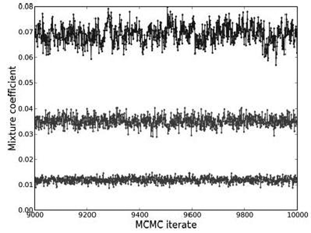
Trace plots for the proportion of the 5th (top), 10th (middle) and 15th (bottom) largest mixture components ( π_i ) over the last 1000 MCMC iterations suggesting convergence.

Choice and interpretation of the number of mixture components

For a given data set, repeatedly fitting the mixture model with increasing numbers of components k can generate useful insights into the suitability of particular values of k. The practical reality of mixture modeling is that, beginning with k = 1,2,…, we expect to see an initial range of values over which the mixture model with increasing numbers of components represents substantial non-normal aspects of the observed data configuration. Increasing k further, however, will eventually begin to add additional components with low probabilities. These components can modestly increase the apparent fit of the model to the data, catering to idiosyncratic features involving a very small number of data points, while often not representing substantively meaningful components. This is an inherent feature of mixture modeling and all attempts to automatically estimate or choose k are affected by it. From a practical perspective, a reasonable strategy utilizes larger numbers of components and bears this "over-fitting" tendency in mind; a fitted model will be inspected and may aim to cut back to components that appear to be substantively relevant.

Methods for treating k as a parameter to be estimated include the Akaike Information Criterion (AIC), Bayes Information Criterion (BIC) and other informational approximations to likelihoods. The graph in Figure 2 is an example of BIC (also known as the Schwartz criterion (17) and is quite typical of what is to be expected in practice. The BIC "optimal" value of k is the maximizing value. Whereas the curve increases quickly from small values of k, indicating that there is indeed mixture structure, it flattens and stays very flat after peaking as additional, low probability components come into play. From the viewpoints of scientific parsimony and relevance, cutting back to smaller values than the absolute peak is generally recommended. In this example, we are interested in the extent to which we can identify biologically meaningful cell subsets present in a human peripheral blood population using a mixture model; the BIC plot suggests 10–15 components as a region where the information curve dramatically flattens off after a steep rise. Though the mode is near 20 components, it is flat between 15–25 and more where multiple low probability components are added. Evaluating and interpreting a mixture model with, say, 15 components may reveal much of the relevant cellular sub-types; repeating the analysis with, say, 20 components, and with due thought to the potential irrelevance of low probability estimated components, may then be viewed as a confirmatory step.

Figure 2.

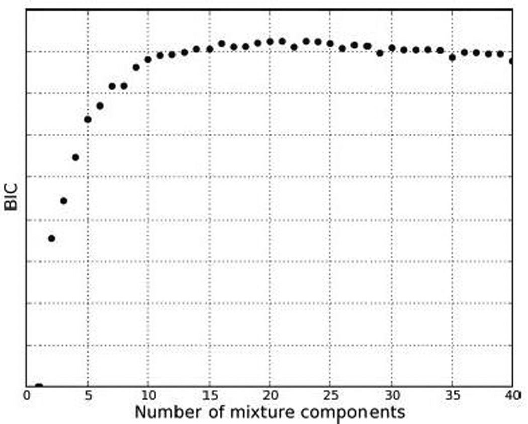
Plot of the BIC against number of mixture components.

Beyond BIC and related methods, formal Bayesian analysis that treats k as a parameter and includes it within the MCMC analysis is available and quite widely used. The main class of models is the class of Dirichlet process mixtures (6,7), nowadays widely used in clustering and mixture deconvolution in machine learning and statistics. Though the use of Dirichlet process mixture models does not obviate the same issue of over-fitting and over-estimation of k, it allows and requires the specification of a prior parameter that can weigh against the data and cut back to smaller values of k. We do not develop this particular approach here, but it can provide a useful exploratory analysis as an initial step that suggests relevant ranges of k.

Results

Identifying cell subsets with mixture components

Filtering irrelevant mixture components

As we have discussed above, in a model fitted with a larger value of k and for purely statistical reasons, very low probability mixture components may be of no interest to an experimentalist. In addition, components that model background noise are typically of no interest. The challenge is then how to filter out such irrelevant mixture components.

A simple definition of a component that models background noise is that the density of that component is below some factor α of the density of a single component model (i.e., using a single multivariate Gaussian to fit the entire data set.) A measure of the volume of a component is given by the square root of the covariance matrix determinant. Using a conservative value of α = 1, if the density of a mixture component is below that of the single component model, that component is rejected as modeling background noise.

Grouping components to form cell subsets

Since the hypersurfaces of constant density for a normal distribution are ellipsoidal, cell subsets with an asymmetrical density may require more than one normal component for a good fit. In other words, a cell subset may be identified with a group of mixture components, rather than a single component.

We assume that a subset consists, by definition, of a single cell type and that its density is unimodal. The density may not be Gaussian, however, and thus may be fit with multiple mixture components as described above. We therefore find the modes in the density by numerical optimization of the mixture density, starting from the means of the mixture components found. Modes that fall outside the range of the data are discarded. While this only detects modes within the convex hull of the component means, and modes that arise from summing overlaps between two or more mixture components will not be detected, such modes do not plausibly correspond to distinct cell subsets and are not considered. Mixture components with a common mode are therefore merged for the purposes of assigning a cell type label.

There is another complication for log-transformed data in that low and negative value fluorescence intensities in any channel will result in the data piling up against an axis. As a consequence, the resulting distribution is markedly non-normal, and typically an extra mixture component is necessary to model such cases. We therefore also merge mixture components that are smeared against an axis with its nearest contiguous neighboring cluster. Doing this, we find that the number of cell subsets is typically smaller than the number of mixture components.

Identifying cell subsets in human peripheral blood

As an example, we describe the procedure for 15 mixture components, which is in the early plateau of the BIC plot shown in Figure 2. After filtering out very low density components (8, 13–15), we are left with 11 mixture components (Figure 3). Of these, it was clear from the FSC/SSC plot that component 5 was debris and 11 consisted of doublets. Components 1 and 4 share a mode, and hence are considered as a single subset. Component 2 clusters together with 1 and 4 but required a separate component because it was smeared against the CD19 axis. Together 1, 2 and 4 evidently form the granulocyte subset. Component 10 is identified as the monocyte subset. Components 3, 6, 9 and 12 appear to be lymphocytes, with 3 being CD3⁺CD4⁺ (CD4 lymphocytes), 6 being CD3⁺CD8⁺ (CD8 lymphocytes) and 9 being CD19⁺ (B lymphocytes). Component 12 was CD3⁺ and CD8⁻ to CD8^dim, and may be an NK cell population. We were unable to identify component 7 (dead cells?), which was negative for CD3, CD4, CD8 and CD19. The final set of putative cell subsets with their frequencies is shown in Table 1. The analysis for 20, 25 and 30 mixture components was very similar, as the additional components mostly represented either noise, events piled up against some axis or multiple components with a common mode. The only essential difference was that with a larger number of components, the component corresponding to 12 was split into at least 2 components, CD8^dim and CD8⁻.

Figure 3.

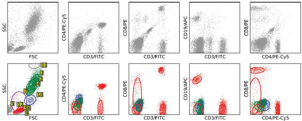
Filtering and identification of mixture components in human peripheral blood. The top row shows the ungated events, while the bottom row shows the mixture components identified, with green for granulocytes, blue for mononuclear cells, red for lymphocytes and maroon for an unclassified component. Mixture components representing aggregates, dead cells and debris in grey are only shown for the FSC/SSC plots in the bottom row. Ellipses and numbered yellow labels on the FSC/SSC plot show the 67% coverage set for each component. Each column is on the same scale.

Table 1.

Identification of mixture groups with putative cell subsets of interest showing proportion of cells in each subset.

Components	Percentage	Classification
1, 2, 4	47.75	Granulocytes
10	4.06	Mononuclear cells
3	11.21	CD3+CD4+ lymphocytes
6	4.99	CD3+CD8+ lymphocytes
9	4.52	B lymphocytes
12	3.53	CD3−CD4−CD8−/dim NK cells

Improving classification accuracy

Thresholding to reduce false positives

The allocation of flow cytometric events to one of the six identified groupings was done by assigning each event to the component with the highest posterior probability. While this procedure minimizes misclassification, we can improve specificity by setting a threshold for the posterior probability. If the highest posterior probability for an event falls below this threshold, the event is not assigned to any component and is instead treated as "uncertain" (Figure 4). This is particularly useful if the purity of the cell subset identified is critical, as for example, in cell sorting applications of flow cytometry.

Figure 4.

Using thresholds to increase specificity. The top panel shows the lymphocyte subsets in which events where the posterior probability of belonging to any lymphocyte component falls below 0.95 have been enlarged. The bottom panel shows the result after filtering out the uncertain events. Most of the uncertainty is with the CD8-negative sub-population of the CD3⁻CD8^−/dim component, which overlaps the unclassified component.

Excluding outliers with coverage sets

Another advantage of Bayesian analysis for flow cytometry is the ability to exclude outliers, events that lie far away from the mean and hence may not be representative of any group. Such outliers can be rejected by filtering out events that fall outside some specified coverage level (or confidence region), which can be easily calculated from the mixture component's covariance matrix. For example, the ellipses corresponding to the 67% confidence regions are shown in the last 4 columns of Figure 3, and any other coverage level desired can just as easily be specified. Unlike the thresholding described above that filters out events which do not obviously belong to a particular group, use of coverage sets filters out events that are in some sense anomalous for the group they belong to.

Manual gating and mixture modeling

When manual gating is used to identify cell subsets, events that do not belong to the cell subset but are fortuitously included may occur since gates are specified only for a one- or two-dimensional slice of the data, which is sometimes corrected by back-gating. Since mixture modeling is intrinsically multivariate, such events are naturally excluded, as only events that are close in all dimensions will belong to the same component, and hence back-gating is unnecessary.

However, manual gating and mixture modeling are not necessarily incompatible. For complex data sets, it may be beneficial to exploit available expertise by first performing manual gating to reduce the size and complexity of the data set, and then doing mixture modeling to identify and clean the remaining subsets.

Validation

Comparison with traditional gating analysis by experts

The NIH Division of AIDS (DAIDS) conducts a proficiency test for clinical flow cytometry laboratories in which the laboratory must prepare peripheral blood samples for flow cytometry, and estimate the frequencies of the following lymphocyte subsets – CD3 total, CD3+CD4+, CD3+CD8+, CD3-CD19+ and CD3-CD(16+56)+. We ran the statistical mixture model on 20 such samples (5 different samples × 4 different preparations) and identified the relevant lymphocyte subsets as described in the manuscript. The frequencies obtained by mixture modeling and expert gating are in close agreement as shown in Table 2. Figure 5 shows the population components identified using the statistical mixture model for a representative patient in the DAIDS data set, with each cell subset tagged with the corresponding frequencies listed in Table 2.

Table 2.

Comparison of lymphocyte subset frequencies obtained using a statistical mixture model and traditional gating by experts. Values shown for each subset are percentages of total lymphocyte events. The CD3+ row is the mean value across all 4 preparations. Frequencies obtained using statistical mixture modeling have a clear background, while pooled frequencies by experts using traditional gating have a light grey background. Values in brackets are the lower and upper quartiles estimated by the group of experts. Samples S1 to S4 are quadruplicate samples from the same donor, sample T1 comes from a different donor. The suffix “A” indicates results obtained using the Automated algorithm, while “E” indicates Expert results.

Sample	S1A	S1E	S2A	S2E	S3A	S3E	S4A	S4E	T1A	T1E
CD3+	75.03	73 (68.3–74)	75.90	74	76.96	74	75.67	74	79.13	79 (78–79)
CD3+CD4+	23.65	23 (22–23.8)	23.31	23	23.94	23	23.01	24	26.26	26 (25–26)
CD3+CD8+	49.23	48 (45–49)	53.12	49	52.49	50	52.20	50	51.49	51 (49–51)
CD3−CD19+	16.19	16 (15.3–21.8)	16.89	16	15.93	16	15.48	14	10.83	11 (10–11)
CD3−CD(16+56)+	9.49	9 (8–10)	9.80	8	7.93	8	10.54	10	8.64	10 (9–11)

Figure 5.

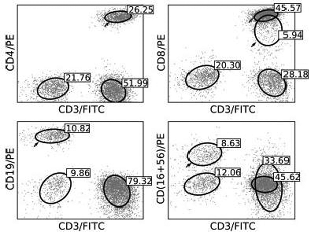
Lymphocyte subset components identified by statistical mixture modeling in the DAIDS samples from donor T. The component(s) arrowed is the target of interest for that sample. Labels show percentage of events in each component as a fraction of total lymphocytes (same as for Table 2).

Classification of a “known” cell mixture and calculation of the recall and precision

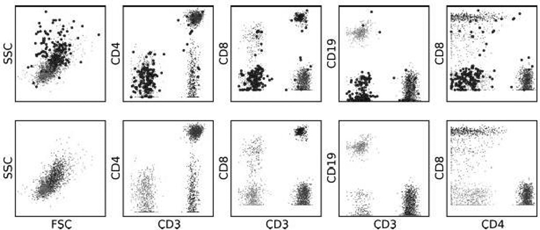
For this analysis, we prepared stained samples of 4 different mouse cell lines (RAW 264.7, JAWS II, CTLL-2 and A20) and ran them individually through the cytometer. Next we mixed them electronically in different proportions to make up a total of 39000 events, and evaluated the accuracy, sensitivity and specificity of the statistical mixture model classification. The flow cytometric profiles of the superimposed pure cell lines after filtering out debris and doublets and the fitted components are shown in Figure 6. The cell densities are clearly not elliptical, and hence multiple mixture components were needed to fit each cell subset. However, with the exception of RAW 264.7, each of the mixture components for that cell line shared a common mode and could therefore be identified with a unique cell line. RAW 264.7 was bimodal, but since this was true even when fitting a pure population, the bimodality indicates that RAW 264.7 cell lines can express two different phenotypes in culture, and both modes were used to identify events belonging to the RAW 264.7 cell line.

Figure 6.

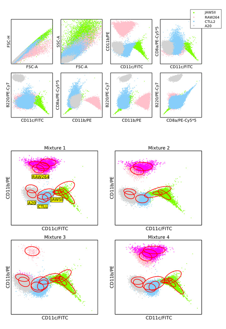
Top panel shows the superimposed flow cytometric profiles of 4 mouse cell lines, showing clear deviation from Gaussianity. Bottom panel shows the statistical mixture model fits to the electronically mixed cell line data for 4 different mixtures projected onto the CD11c/CD11b axes. Components sharing a common mode are colored identically. Note that the RAW 264.7 cell line is bimodal – this is true even when fitting a pure RAW 264.7 population alone, and we have therefore used both modes in our calculations.

Table 3 shows the estimated percentages of each of the cell lines compared with the known mixing proportions for 4 different mixtures. Mixture 1 had equal proportions of all cell lines, mixture 2 had 40% of JAWS II and A20 each and 10% of RAW 264.7, mixture 3 had 33% each of JAWS II, CTLL-2 and A20 and 1% of RAW 264.7 and mixture 4 had randomly chosen mixing proportions. The results for mixture 3 shows mixture models can resolve relatively small components (1% for RAW 264.7).

Table 3.

Actual and estimated percentages of the 4 cell lines using modal clusters. The estimated percentages do not necessarily sum up to 100 as low density components that do not share a mode with any other components have been filtered.

	Mix 1	Estimate	Mix 2	Estimate	Mix 3	Estimate	Mix 4	Estimate
RAW 264.7	25.0	24.94	10.0	9.98	1.00	0.74	22.14	22.30
JAWS II	25.0	24.84	40.0	40.47	33.0	33.31	32.14	32.02
CTLL-2	25.0	25.39	10.0	9.37	33.0	32.68	18.54	18.53
A20	25.0	24.83	40.0	40.18	33.0	32.95	27.19	26.87

In table 4, the number of correctly and incorrectly classified events was used to calculate the sensitivity, specificity, positive predictive value (PPV) and negative predictive value (NPV) of the algorithm for mixture 1, using the following standard definitions

• Sensitivity = # True Positive / (# True Positive + # False Negative)

• Specificity = # True Negative / (# True Negative + # False Positive)

• PPV = # True Positive / (# True Positive + # False Positive)

• NPV = # True Negative / (# True Negative + False Negative)

Table 4.

Binary classification table for JAWS II cells for Mixture 1. The values for the other cell lines are similar (not shown). PPV is positive predictive value, NPV is negative predictive value.

II JAWS	True	False
Positive	9677	77	PPV= 99.21%
Negative	73	29173	NPV = 99.75%
	Sensitivity = 99.25%	Specificity = 99.74%

Table 5 shows a confusion matrix, in which columns represent the predicted classification of the indicated cell line, while rows represent the true classification. For example, the first row of Table 5 shows that of the 9750 JAWS II events in Mixture 1, 9677 were correctly identified while 73 were incorrectly classified as CTLL-2 cells.

Table 5.

Confusion matrix for Mixture 1. Rows show true classification while columns show predicted classification.

	JAWS II	RAW 264.7	CTLL-2	A20
JAWS II	9677	0	73	0
RAW 264.7	0	9748	2	0
CTLL-2	77	0	9673	0
A20	0	0	0	9750

Discussion

We have shown in this manuscript that Bayesian mixture models can extract biologically meaningful components (cell subsets) from flow cytometric data, by defining putative cell subsets as groups of mixture components fitting the following criteria:

1. each component must have a density greater than some threshold to distinguish it from noise; a reasonable threshold density is the density of a single multivariate normal fitted to the same data set

2. each component must have a well-conditioned covariance matrix

3. the components, taken together, have a single mode

It may also be necessary to merge components that result from events piling up against an axis, typically resulting from log transformation of the data. This is an artifact of the log transform, and disappears with linear FCS 3.0 data using the hyperlog (18) or logicle (19) transforms (data not shown).

Using these putative cell subsets, we show that the accuracy of event classification can be improved by thresholding on the posterior density of each event, or by selecting events from a smaller coverage set. Critically, this analysis also provides us with a robust statistical model of flow cytometric data that can potentially be used for the rigorous statistical comparison of two or more flow cytometric data sets. If flow cytometric data can be normalized in a standardized fashion, it should also be possible to build up a training set of flow cytometric samples, allowing future automated classification of cell subsets in a sample, as well as classification of entire data samples (e.g. as normal or abnormal).

In the traditional analysis of flow cytometry, the choice of which sequence of markers to gate on and where to draw the gates depends on expertise and it is difficult to replicate cell subset identification and quantitation across different laboratories. The problem is compounded with increasing number of colors, since the number of possible gating sequences rises rapidly with the number of markers used. The process of manual compensation and gate delineation is also extremely time-consuming, and hence a major cost factor in large scale clinical flow cytometric analysis.

It is clear that some of the complexity of flow cytometric analysis arises from the use of 1- or 2-D tools to analyze data that exist in higher-dimensional parameter space. The use of appropriate multivariate statistical approaches would therefore result in a simpler workflow and may also offer greater accuracy in the quantitation of cell subsets, since projections in 2-D that cannot be resolved may often be separable with a higher dimensional partition surface. For these reasons, several automated heuristic-based methods (e.g. discriminant analysis, neural networks and support vector machines) have been suggested for the clustering and classification of flow cytometry data.

However, we believe that a more principled model-based approach using mixture models has many benefits - for example, we can use the model to detect anomalous events, determine rejection criteria to minimize mis-classifications and even construct models for combining different sets of data. In addition, the analysis of mixtures using current computational statistical technology is automatic, and will apply in as many dimensions as we have markers. Unlike the previous approaches outlined above, statistical mixture methods can also more easily exploit biological expert knowledge in the specification of priors. Furthermore, calculation of estimation intervals and the assessment of uncertainty in the posterior probability of belonging to groups is simple with a Bayesian approach, allowing us to control the purity of extracted cell subsets naturally. Importantly, a model-based approach allows increasingly sophisticated models to be constructed so as to better capture data constraints (e.g. hierarchical cluster structure), which will result in more accurate and efficient classification schemes.

Bayesian mixture models can be extended to an arbitrary number of dimensions, and we are actively researching its utility for the analysis of polychromatic flow cytometry. In practice, however, several challenges have to be overcome for this to be practical. We have described a simple but adequate strategy for determining the number of components, by simply adding components until the contribution of the last added component is negligible. With a larger number of dimensions and a corresponding increase in the number of mixture components necessary, such an approach may be too inefficient. More advanced sampling methods can estimate the number of components directly. In high dimensions, it is also critical to develop more efficient samplers, and advances in this direction include gradient optimization and the combination of variational optimization with MCMC.

We believe that Bayesian models are a promising approach to the automated or semi-automated analysis of flow cytometric data. With the increasing dimensionality and volume of flow cytometric data being generated, such an approach is likely to prove ever more useful and necessary.

References

- 1.Cormack RM. A Review of Classification. Journal of the Royal Statistical Society. Series A (General) 1971;134:321–367. [Google Scholar]
- 2.Maecker HT, Rinfret A, D'Souza P, Darden J, Roig E, Landry C, Hayes P, Birungi J, Anzala O, Garcia M, et al. Standardization of cytokine flow cytometry assays. BMC Immunol. 2005;6:13. doi: 10.1186/1471-2172-6-13. [DOI] [PMC free article] [PubMed] [Google Scholar]
- 3.Tarnok A. A focus on automated recognition. Cytometry A. 2007;71(10):769–770. doi: 10.1002/cyto.a.20472. [DOI] [PubMed] [Google Scholar]
- 4.Robert CP. Mixtures of distributions: Inference and estimation. Markov Chain Monte Carlo in Practice. 1996:441–464. [Google Scholar]
- 5.Titterington D, Smith AFM, Makov U. Statistical Analysis of Finite Mixture Distributions. John Wiley & Sons; 1985. [Google Scholar]
- 6.West M. Modelling with mixtures (with discussion) Bayesian Statistics 4. 1992:503–524. [Google Scholar]
- 7.Escobar MD, West M. Bayesian density estimation and inference using mixtures. Journal of the American Statistical Association. 1995;90:577–588. [Google Scholar]
- 8.Turner DA, West M. Statistical analysis of mixtures applied to postsynaptic potential fluctuations. Journal of Neuroscience Methods. 1993;47:1–23. doi: 10.1016/0165-0270(93)90017-l. [DOI] [PubMed] [Google Scholar]
- 9.West M. Hierarchical mixture models in neurological transmission analysis. Journal of the American Statistical Association. 1997;92:587–606. [Google Scholar]
- 10.Turner DA, Chen Y, Isaac J, West M, Wheal HV. Heterogeneity between non-NMDA synaptic sites in paired-pulse plasticity of CA1 pyramidal neurons in the hippocampus. Journal of Physiology. 1997;500:441–461. doi: 10.1113/jphysiol.1997.sp022032. [DOI] [PMC free article] [PubMed] [Google Scholar]
- 11.Lavine M, West M. A Bayesian method for classification and discrimination. Canadian Journal of Statistics. 1992;20:451–461. [Google Scholar]
- 12.Robert CP. Markov Chain Monte Carlo in Practice. Chapman & Hall; 1996. [Google Scholar]
- 13.Gelfand AE, Smith AFM. Sampling-Based Approaches to Calculating Marginal Densities. Journal of the American Statistical Association. 1990;85:398–409. [Google Scholar]
- 14.de Hoon MJ, Imoto S, Nolan J, Miyano S. Open source clustering software. Bioinformatics. 2004;20(9):1453–1454. doi: 10.1093/bioinformatics/bth078. [DOI] [PubMed] [Google Scholar]
- 15.Nelder JA, Mead R. A simplex method for function minimization. The Computer Journal. 1964;7:308–313. [Google Scholar]
- 16.Cowles MK, Carlin BP. Markov Chain Monte Carlo Convergence Diagnostics: A Comparative Review. Journal of the American Statistical Association. 1996;91(434):883–904. [Google Scholar]
- 17.Schwarz G. Estimating the Dimension of a Model. The Annals of Statistics. 1978;6(2):461–464. [Google Scholar]
- 18.Bagwell CB. Hyperlog-a flexible log-like transform for negative, zero, and positive valued data. Cytometry A. 2005;64(1):34–42. doi: 10.1002/cyto.a.20114. [DOI] [PubMed] [Google Scholar]
- 19.Parks DR, Roederer M, Moore WA. A new "Logicle" display method avoids deceptive effects of logarithmic scaling for low signals and compensated data. Cytometry A. 2006;69(6):541–551. doi: 10.1002/cyto.a.20258. [DOI] [PubMed] [Google Scholar]
- 20.Green PJ, Richardson S. Modelling heterogeneity with and without the Dirichlet process. Scandinavian Journal of Statistics. 2000;28:355–375. [Google Scholar]
- 21.Richardson S, Green PJ. On Bayesian analysis of mixtures with an unknown number of components. Journal of the Royal Statistical Society, Series B. 1997;59:731–792. [Google Scholar]
- 22.Stephens M. Bayesian analysis of mixture models with an unknown number of components--an alternative to reversible jump methods. Ann. Statist. 2000;28(1):40–74. [Google Scholar]
- 23.Qin Z, Liu JS. Exploring Hybrid Monte Carlo in Bayesian Computation. 2001 [Google Scholar]
- 24.Freitas ND, Russell S. Variational MCMC. UC Berkeley: 2001. [Google Scholar]
Associated Data
This section collects any data citations, data availability statements, or supplementary materials included in this article.