

Abstract
A method is presented for high spatial and temporal resolution 3D contrast-enhanced magnetic resonance angiography. The overall technique involves a set of interrelated components suited to high-frame-rate angiography, including 3D cylindrical k-space sampling, angular undersampling, asymmetric sampling, sliding window reconstruction, pseudorandom view ordering, and a sliding subtraction mask. Computer simulations and volunteer studies demonstrated the utility of each component of the technique. Angiograms of one hemisphere of the intracranial vasculature were acquired with a pixel size of 1.1 × 1.1 × 2.8 mm and a frame rate of 0.35 sec based on a temporal resolution of 3.5 sec. Such a 3D time-resolved, or “4D,” technique has the potential to noninvasively acquire diagnostic quality images of certain anatomic regions with a frame rate fast enough to not only ensure the capture of an uncontaminated arterial phase, but even demonstrate contrast bolus flow dynamics. Clinical applications include noninvasive imaging of arteriovenous shunting, which is demonstrated with a patient study.
Keywords: magnetic resonance angiography, contrast, time-resolved, radial imaging, ordering, subtraction
Since the introduction of contrast-enhanced MR angiography (CE-MRA) (1), the technique has evolved to achieve higher image quality in terms of spatial resolution and signal-to-noise ratio (SNR). Recently, much effort has been directed at trying to increase temporal resolution so that a multiphase acquisition will always have an uncontaminated arterial phase volume, eliminating the need for contrast bolus timing. Further, time-resolved CE-MRA, if fast enough, can follow the first pass of contrast through the vasculature to show flow dynamics, which is necessary in certain clinical scenarios such as arteriovenous shunting, retrograde flow, or delayed vessel enhancement. Currently, x-ray digital subtraction angiography (DSA) (2) is the clinical standard for time-resolved angiography. However, unlike MRI, x-ray DSA utilizes ionizing radiation and nephrotoxic contrast material and carries the small but definite risk of introducing embolic material. In addition, MRI can provide true 3D imaging, not just projection imaging, in order to visualize the complex 3D geometry of blood vessels. The combination of 3D and time-resolved imaging is also known as “4D” imaging.
CE-MRA would be a viable option for time-resolved angiography if the SNR, spatial resolution, and temporal resolution were sufficient for the clinical problem. However, there is an inherent trade-off between these three parameters in MRI, given a fixed field-of-view (FOV). In recent times, the research community has developed a great number of novel acceleration, or undersampling, techniques to increase spatial and temporal resolution at the expense of SNR. These techniques can be broadly classified as temporal and/or spatial undersampling. Temporal undersampling involves the estimation of missing k-space samples from past and future acquired samples at the same spatial frequency. The “sliding window” technique was among the first acceleration strategies to be developed (3,4). It involves the repeated acquisition of N segments of a whole volume such that frames can be formed by any contiguous set of N segments. The frame rate is increased by N, but the data are low-pass filtered in the temporal dimension. The “keyhole” technique first acquires a high-resolution volume, and subsequently only updates the low-frequency information, where most of the image lies (5). BRISK (6), TRICKS (7), and STBB analysis/acquisition (8) techniques built on previous ideas by acquiring the central k-space lines at a higher sampling rate than peripheral lines. Spatial undersampling techniques involve the estimation of missing k-space lines from other acquired lines at different spatial frequencies in the same time frame. One technique, in use for many years now, involves the asymmetric sampling of k-space. Spatial frequencies higher than a certain threshold are not acquired on one side of k-space, and the missing data are either zero-filled or extrapolated. This concept can be extended by applying it in multiple dimensions for large overall undersampling factors. Parallel imaging is comprised of a group of techniques which use multiple receiver coils to speed up acquisition. The SMASH technique was one of the first described (9), and it has matured into GRAPPA (10), which is presently state-of-the-art. Another class of parallel imaging approaches is based on SENSE (11). Alternative k-space trajectories may have their own specific undersampling techniques. For example, the radial trajectory can be angularly undersampled (12,13). Combinations of temporal and spatial undersampling, such as PR-TRICKS (14), k-t SENSE (15), and TSENSE (16) can be used, and may even be preferable to a single acceleration technique alone.
Another concern in developing a time-resolved CE-MRA sequence relates to ordering the acquisition of k-space lines. Since lines are acquired in a serial fashion, the passage of contrast causes a modulation of the signal according to the order in which the lines are acquired (17). Better ordering methods, such as elliptical centric ordering (18), will minimize the artifact associated with serial measurement.
Subtraction for CE-MRA is conventionally performed using a single time frame as the mask. The mask is chosen at a time prior to the arrival of contrast. For timed CE-MRA, the acquisition typically consists of three volumes: the mask, arterial phase, and venous phase. Time-resolved acquisitions open up a new set of applications and, therefore, the way in which subtraction is performed may need to be reconsidered.
In the context of time-resolved imaging, this article attempts to address these issues of undersampling, ordering, and subtraction with a CE-MRA technique combining a 3D radial trajectory (cylindrical sampling), sliding window reconstruction, pseudorandom ordering, and a sliding subtraction mask. The goals are to demonstrate with simulations and healthy volunteer studies that 1) for the sliding window reconstruction, the artifact associated with the radial trajectory is less severe than that for the spin-warp trajectory (Cartesian sampling); 2) proper ordering is essential when combining the radial trajectory with the sliding window method; and 3) the sliding mask subtraction technique better depicts the wash-in and wash-out of contrast than conventional subtraction.
MATERIALS AND METHODS
Sequence Design
To determine spatial and temporal resolution requirements of the 4D CE-MRA pulse sequence, the intracranial catheter-directed x-ray angiograms of 17 consecutive patients with either intracranial arteriovenous malformations (AVMs) or fistulae (AVFs) were studied retrospectively. In many patients, multiple feeding arteries existed, so a total of 44 feeding arteries were examined and their diameters were found to be 2.39 ± 0.96 mm with a range of 1.0–4.8 mm. From this study we determined that a spatial resolution of at least 1 mm was desirable. A frame rate of 2–3 frames/sec was necessary to catch a pure arterial phase, depending on the blood flow through the AVM or AVF.
For the 4D CE-MRA pulse sequence, FLASH (19) contrast is used with a 3D radial trajectory (cylindrical sampling) (13,14). Asymmetric sampling is applied along the read-out (kr) dimension as well as along the through-plane (kz) phase-encoding dimension. Angular undersampling is applied such that the number of projections/views, Nθ, is less than that of the fully sampled case, Nθ < πNr/2, where Nr is the number of read-out points. A 2D (in-plane dimensions) diagram of the radial trajectory with read-out asymmetric sampling and angular undersampling is shown in Fig. 1a. Figure 1b extends k-space to 3D by applying phase encoding in the z dimension.
FIG. 1.
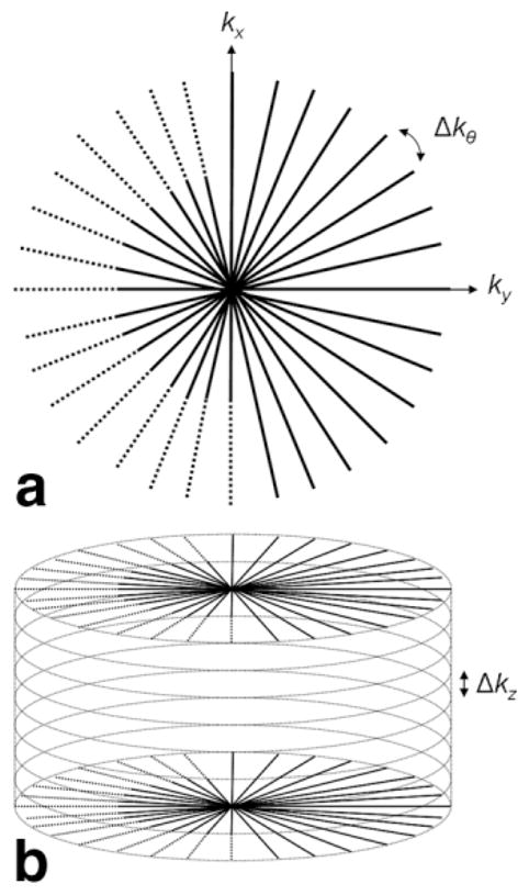
(a) Diagram of radial trajectory in 2D k-space. Δkθ = 2π/Nθ. (b) Extension of (a) to 3D where k-space is sampled on a cylindrical grid. The origin of k-space is defined to be at the center of the cylinder.
For image reconstruction, missing data due to asymmetric sampling are zero-filled. The reconstructed frame rate is increased over the acquired frame rate with the sliding window method by a factor of fSW by segmenting the acquisition into fSW segments and forming time frames from all contiguous sets of fSW segments. As a result, for Nrep. repetitions, fSW(Nrep.-1)+ 1 time frames are produced.
Pseudorandom Ordering
The ordering algorithm was designed with the following criteria:
Through-plane/z-dimension phase-encodes are looped inside views/projections, with z phase-encodes ordered in a centric fashion. In this way, the center of k-space is acquired often and at regular intervals, and the + kz and −kz components of a spatial frequency are acquired at approximately the same time (except for certain higher kz samples, which are zero-filled due to asymmetric sampling).
k-space is segmented in an interleaved manner, where Nsegments is the number of segments. Lines belonging to a segment are spaced Nsegments lines apart. A single segment is updated for every consecutive time frame generated by the sliding window reconstruction. In other words, Nsegments is equal to the sliding window factor, fSW.
Within a segment/time frame, the set of views is chosen to be distributed evenly around a circle in the kx-ky plane. This is to prevent “bunching” of views. (This criterion simply describes the set of angles; their acquisition order is described next.)
Within a segment/time frame, views are not acquired linearly (i.e., kθ is not incremented by Δkθ). Rather, the angle between consecutive views is fθ· Δkθ, where fθ is a factor to spread out consecutive views in the angular dimension.
Similarly, segments are not acquired linearly, and a factor, fsegment, prevents “bunching” of consecutive segments in the angular dimension.
In general, this ordering method tries to distribute samples in space and time, so that artifact associated with acquiring bunched samples will be minimized (20,21). The order of views can be represented by a sequence, nθ, ranging from 1 to the total number of views, Nθ, where each number in the sequence corresponds to a view at angle πnθ/Nθ. The line reordering algorithm can be expressed as a one-to-one mapping of the linearly ordered sequence, nθ, to the reordered sequence, r[nθ]:
| [1] |
The mod(x,y) function, where x and y are integers, returns the remainder after division of x by y. The floor(x) function rounds down to the nearest integer. The first term inside the outermost mod function controls the order of lines within a segment, and the second term factors in the segment number. Again, a full set of z phase-encodes are acquired at every view before continuing to the next view. Asymmetric sampling is not considered in this equation for the sake of simplicity. Although the ordering is indeed calculated by an analytic expression, the ordering appears quite random superficially and, therefore, the term “pseudorandom” is used. Plots of view number, nθ, versus view angle for linear and pseudorandom ordering are shown in Fig. 2.
FIG. 2.

Plots of view number versus view angle for two different ordering techniques (128 views). (a) Linear ordering. (b) Pseudorandom ordering with 16 segments, fθ = 5, fsegment = 9.
As a result of the pseudorandom ordering, the center of k-space is sampled every Nz · fAS,z · TR ms, where Nz is the number of z-encodes and fAS,z is the asymmetric sampling factor in the through-plane dimension. The scan time for one complete 3D volume is NΘ · Nz · fAS,z · TR ms.
Sliding Mask Subtraction
Following image reconstruction with the sliding window technique, magnitude subtraction images are generated by subtracting each volume by the volume acquired a certain amount of time prior, called the subtraction lag time. More specifically, the lag time is an adjustable parameter specifying the time between the beginnings of the minuend and subtrahend (mask) image acquisitions. (The minuend minus the subtrahend forms the difference image.) The sliding mask subtraction procedure is diagrammed in Fig. 3, with comparison to conventional subtraction. Any negative values in the subtracted images are truncated to 0 in order to prevent regions in which recent enhancement has subsided, such as at the tail of a bolus, from appearing less intense than background. Maximum intensity projections (MIPs) are calculated from the subtracted volumes for visualization in 2D.
FIG. 3.

(a) Initial mask and (b) sliding mask subtraction with sliding window reconstruction. The paired numbers, [a,b], represent the data associated with the ath set of lines acquired for the bth complete volume. One new set of lines is updated for every new time frame. a ranges from 1 to fSW, and when fSW = Nsegments, a also indicates the ath segment. The subtrahend and minuend are formed by contiguous sets of lines, and the angiogram is formed by subtracting the subtrahend from the minuend. The subtraction lag time is defined as the time between the beginnings of the minuend and subtrahend.
The sliding mask subtraction can also be thought of as an approximation to the time-derivative of the signal-time curve at each pixel. As the subtraction lag time is minimized, the approximation becomes better. Contrast-to-noise (CNR) in sliding mask subtraction images is dependent on both the shape of the signal-time curve and the lag time.
Simulations
Computer simulations were performed to compare the sliding window method with the spin-warp trajectory versus the radial trajectory. In addition, for the radial trajectory the pseudorandom ordering technique was compared with conventional linear ordering. The simulations modeled a bolus of contrast material of length l traveling through a straight blood vessel of width w. Starting at position y0, the bolus travels with speed v. If the blood vessel can be approximated with a square cross-section, the truth image, i, as a function of space (x, y, z) and time (t) variables,
| [2] |
is separable with a 3D spatial Fourier transform, I, given by:
| [3] |
k-space can also be written in cylindrical coordinates:
| [4] |
Note that the motion of the bolus through the vessel is accounted for in k-space by simply a phase shift. Clearly, the model is limited to a certain degree in that the vessel has a rectangular cross-section and bolus instantly arrives and vanishes. The analytic expression of the moving object in the spatial frequency domain was sampled with real sequence parameters to simulate the different types of acquisitions under consideration. Images were reconstructed and postprocessed, then analyzed qualitatively. Simulation parameters were chosen based on the previously described study to determine spatial and temporal resolution requirements for angiography of intracranial AVMs and AVFs. The blood vessel width was 4 mm (in x and z dimensions), and the contrast bolus was 16 mm in length (in y dimension) and traveled at a speed of 5.2 mm/sec. The sequence parameters held constant were as follows: FOV: 128 × 128 × 16 mm, image matrix: 128 × 128 × 16, pixel size: 1.0 × 1.0 × 1.0 mm, four phases, temporal resolution: 6.1 sec, sliding window factor: 16, frame rate: 0.38 sec, TR = 3 ms. Spin-warp acquisitions were ordered with the elliptical centric method, in which lines were acquired in order of their increasing perpendicular distance from the center of k-space. The frame rate was in no way associated with any features of the elliptical centric ordering. Simulations were performed with the read-out direction set both parallel and perpendicular to the direction of blood flow. The following parameters were used for the pseudorandom ordering method: 8 views/segment, 16 segments, fθ: 5, fsegment: 9. Cylindrically sampled acquisitions were regridded prior to computing the inverse discrete Fourier transform. The regridding algorithm was programmed with a three-sample Kaiser-Bessel interpolator and a linear density compensation function (22) without correction in sampling density due to asymmetric sampling. All computation was performed with Matlab (MathWorks, Natick, MA) software. Images were visually inspected to compare signal fidelity and artifact distribution.
Volunteer Studies
Images were acquired from nine healthy volunteers on a 1.5T whole body MR scanner (Avanto, Siemens Medical Solutions, Erlangen, Germany) with an 18-channel head/neck coil array. The 3D multiphase FLASH pulse sequence with a radial trajectory acquired a lateral view of the intracranial vasculature in one hemisphere, including the sagittal sinus. Sequence parameters were as follows: FOV: 220 × 220 × 75 mm, Nr/Nθ/Nz = 192/96/27, image matrix: 192 × 192 × 27, pixel size: 1.1 × 1.1 × 2.8 mm, 10 phases, temporal resolution: 3.5 sec, sliding window factor (fSW): 10, number of segments (Nsegments): 10, frame rate: 0.35 sec, TR/TE: 2.4/0.9 ms, receiver bandwidth: 1000 Hz/pixel (sampling period: 5.2 μs), flip angle: 25°, read-out/through-plane asymmetric sampling factors (fAS,r/fAS,z): 75%/75%, angular undersampling factor (2Nθ/πNr): 32%. The temporal resolution can be calculated with the following formula:
| [5] |
For a certain volunteer, images were either acquired with pseudorandom ordering or linear ordering. Images were reconstructed and postprocessed offline in Matlab. Both conventional and sliding mask subtraction images were calculated, followed by sagittal MIPs (along the z direction to achieve maximum in-plane spatial resolution). A 0.1 mmol/kg dose of a gadolinium-based contrast agent (Magnevist, Berlex, Wayne, NJ) with a 20-mL saline flush was administered with a power injector (Spectris Solaris, Medrad, Indianola, PA) in an antecubital vein at an injection rate of 4.0 ml/sec, starting simultaneously with the imaging protocol. The study was approved by our Institutional Review Board.
To compare signal versus time curves for the conventional and sliding subtraction techniques, regions-of-interest (ROIs) were drawn at the same locations in the images generated by the two techniques. An arterial ROI covered the cavernous segment of the internal carotid artery, and a venous ROI covered the most superior portion of the superior sagittal sinus. Next, the effect of varying the lag time was studied for the sliding mask subtraction operation. The artery-background, vein-background, and artery-vein CNR were calculated at the peak arterial, peak venous, and peak venous phases, respectively, for lag times of 2.5, 5.0, 7.5, 10, 12.5, 15 sec. The peak venous phase was chosen for the artery-vein CNR calculation to assess how much arterial signal is suppressed by the time veins reach peak enhancement. In addition, a metric was derived to measure the overlap of arterial and venous signal versus time curves, called the “overlap integral,” O:
| [6] |
where A[n] and V[n] are the discrete-time arterial and venous signals, N is the total number of samples, and n and m are sample number indices. The overlap integral can be visualized as the area under the curve defined by the lesser of the arterial and venous signals at each time-point. A smaller overlap integral indicates better temporal separation of arterial and venous signals. The arterial and venous signals are each first normalized such that the area under each curve is 1. Arterial and venous signal ROIs were drawn at the same locations described previously. The image analysis software consisted of a custom graphical user interface developed in the Matlab environment. For artery-background CNR, vein-background CNR, artery-vein CNR, and overlap integral, two-tailed paired t-tests were performed to determine whether mean values were significantly different between the initial and sliding mask subtraction techniques. The comparison was repeated for every lag time.
Patient Study
To demonstrate the utility of this noninvasive, high-framerate 4D angiography technique, a patient with a Spetzler-Martin Grade II right posterior AVM confirmed on x-ray DSA was imaged preoperatively on a 3.0T whole body MR scanner (Trio, Siemens Medical Solutions) with a 12-channel head/neck coil array. The imaging protocol remained the same as that for the volunteer studies, except to accommodate the greater specific absorption rate at higher field the TR was increased to 3.9 ms. In addition, fewer z phase-encodes (24) with greater thickness (3.1 mm) were prescribed, resulting in a temporal resolution of 5.0 sec and a frame rate of 0.5 sec. X-ray DSA and MRA images of the feeding artery at the peak arterial frame were compared qualitatively.
RESULTS
Simulations
Figure 4 displays the results of the simulations, comparing consecutive frames from (Fig. 4a) the truth images, sampled with infinitesimally small temporal resolution; (4b) the spin-warp trajectory with elliptical centric ordering and the read-out direction parallel to the direction of blood flow; (4c) the spin-warp trajectory with elliptical centric ordering and the read-out direction perpendicular to the direction of blood flow; (4d) the 3D radial trajectory with z phase-encodes looped inside views, centric ordering of z phase-encodes, and linear ordering of views; and (4e) the 3D radial trajectory with z phase-encodes looped inside views, centric ordering of z phase-encodes, and pseudorandom ordering of views. Although acquisitions were 3D, 2D MIPs are shown. The direction of flow is from left to right. Note the difference in artifact between the three techniques. In Fig. 4b the bolus appears artificially spread out along the direction of travel, and there is ringing in the perpendicular direction. The artifact varies from frame to frame depending on which spatial frequencies are being updated. In Fig. 4c the bolus exhibits ringing along the direction of travel. In Fig. 4d the bolus is less spread out along the direction of travel, but still somewhat blurred. Curved lines emanate from the bolus, and the artifact appears time-dependent. In Fig. 4e the bolus is blurred along the direction of travel, similar to Fig. 4d; however, the curved artifacts are no longer present. Notice that dim artifact is spread out evenly around the bolus. The appearance of the bolus does not seem to change in time.
FIG. 4.

Computer simulations of the passage of a bolus of contrast through a blood vessel using different acquisition techniques. All images are MIPs of a 3D acquisition, and each image series consists of consecutive time frames (moving left to right) at the same points in time. The direction of blood flow is from left to right. The temporal resolution is 0.38 sec. (a) The truth image. (b) The spin-warp trajectory with elliptical centric ordering and the read-out direction parallel to the direction of blood flow. (c) The spin-warp trajectory with elliptical centric ordering and the read-out direction perpendicular to the direction of blood flow. (d) The 3D radial trajectory with linear ordering of views. (e) The 3D radial trajectory with pseudorandom ordering of views.
Volunteer Studies
A typical intracranial CE-MRA using the proposed 4D acquisition is shown in Fig. 5, with conventional initial mask subtraction, and Fig. 6, with sliding mask subtraction. The same dataset was used for each type of subtraction. Image quality varied little across volunteers, as shown by later analysis. The acquisition follows the first pass of the contrast bolus through the intracranial circulation. Although difficult to show in this written report, the frame rate is sufficiently fast for the frames to appear fluid when played in cine mode at the physiologic frame rate. Comparing the initial and sliding mask subtraction techniques, early time frames appear similar. Later time frames, such as during venous enhancement, show exclusively venous enhancement in the sliding mask subtraction images. Figure 7 illustrates the effect of choosing linear view ordering, where successive lines are bunched together. Upon close inspection, notice that the images are updated in a nonuniform fashion, where the updated region sweeps in a circular motion around the center of the image. Images are not updated fast enough to keep up with the passing bolus. Also note the prominent streak artifact coming off the superior sagittal sinus. Signal versus time curves for arterial and venous ROIs drawn from Figs. 5 and 6 are shown in Fig. 8. For the sliding subtraction technique, note the sharper signal peak and the well-defined separation between arterial and venous curves.
FIG. 5.

Typical intracranial CE-MRA with the 4D acquisition and conventional initial mask subtraction. Images are sagittal subtracted MIPs. Pixel size: 1.1 × 1.1 × 2.8 mm, frame rate: 0.35 sec. Windowing is automatically adjusted dynamically to suit the SNR of the frame. (a) Time series mosaic of every other time frame. (b) Selected arterial phase image, magnified. (c) Selected venous phase image, magnified.
FIG. 6.

The same acquisition as in Fig. 4 with sliding mask subtraction. Images are sagittal subtracted MIPs. Pixel size: 1.1 × 1.1 × 2.8 mm, frame rate: 0.35 sec. All images are at the same time points as in Fig. 4. (a) Time series mosaic of every other time frame. (b) Selected arterial phase image. (c) Selected venous phase image, magnified.
FIG. 7.

Typical 4D radial sliding window intracranial CE-MRA with linear view ordering. (a) Time series mosaic of every other time frame. (b) Selected time frame highlighting the fact that the image is not uniformly updated. Here, notice that a more proximal portion of the superior sagittal sinus appears to enhance before a more distal segment (arrows).
FIG. 8.

Representative signal versus time curves for arterial and venous ROIs taken from images produced by (a) initial subtraction or (b) sliding subtraction of the same dataset. Maximum signal has been normalized to 1. The arterial ROI included the cavernous segment of the internal carotid artery, and the venous ROI consisted of the most superior portion of the superior sagittal sinus.
Table 1 lists the results of the comparison between the conventional and sliding subtraction techniques, and the results are displayed graphically in Fig. 9. For each CNR study the CNR increased as a function of lag time. For artery-background and vein-background contrast, the two techniques exhibited significantly different (P < 0.05) CNR at all lag times except 15 sec. For artery-vein contrast, the initial mask subtraction CNR was significantly different from that of sliding mask subtraction at lag times of 2.5, 12.5, and 15 sec. For the overlap integral study, values were significantly different in all cases, with a minimum at ≈ 10 sec.
Table 1.
Mean ± Standard Deviation Artery-Background CNR, Vein-Background CNR, Artery-Vein CNR, and Overlap Integral for Volunteer Studies of Both the Initial Mask Subtraction Technique and the Sliding Mask Subtraction Technique with Varying Lag Times
| CNR |
Overlap integral | |||
|---|---|---|---|---|
| Artery-background | Vein-background | Artery-vein | ||
| Initial mask | 95.6 ± 20.5 | 94.3 ± 20.9 | 57.3 ± 19.2 | 0.697 ± 0.050 |
| Sliding mask | ||||
| 2.5 sec lag time | 30.0 ± 7.7 (P = 0.0005*) | 21.8 ± 5.2 (P = 0.0037*) | 20.0 ± 4.0 (P = 0.0073*) | 0.588 ± 0.062 (P = 0.0207*) |
| 5.0 | 54.2 ± 12.6 (P = 0.0005*) | 42.3 ± 9.7 (P = 0.0003*) | 39.8 ± 8.2 (P = 0.6960) | 0.545 ± 0.068 (P = 0.0050*) |
| 7.5 | 72.7 ± 18.7 (P = 0.0047*) | 60.3 ± 13.5 (P = 0.0041*) | 56.1 ± 10.6 (P = 0.4272) | 0.537 ± 0.066 (P = 0.0021*) |
| 10.0 | 87.1 ± 22.3 (P = 0.0256*) | 74.2 ± 16.6 (P = 0.0226*) | 66.7 ± 13.5 (P = 0.1271) | 0.533 ± 0.064 (P = 0.0001*) |
| 12.5 | 92.2 ± 21.5 (P = 0.0245*) | 83.7 ± 18.3 (P = 0.0269*) | 73.8 ± 15.6 (P = 0.0054*) | 0.543 ± 0.062 (P = 0.0003*) |
| 15.0 | 94.7 ± 21.0 (P = 0.0836) | 90.2 ± 19.0 (P = 0.0548) | 76.9 ± 15.7 (P = 0.0261*) | 0.561 ± 0.062 (P = 0.0041*) |
P-values are the result of a two-tailed paired t-test on the difference in values between the initial mask subtraction technique and each of the individual sliding mask subtraction results.
P-value significant at 5% level.
FIG. 9.

The mean (a) artery-background, (b) vein-background, and (c) artery-vein CNR and (d) overlap integral values for the initial mask subtraction technique (indicated by “initial”) compared to the sliding mask subtraction technique with differing subtraction lag times.
Patient Study
The arterial phase x-ray DSA and MRA for the AVM patient are compared in Fig. 10. The spatial resolution of the x-ray DSA is 0.1 mm in-plane, and the temporal resolution is 3 frames/sec. Thus, the x-ray DSA’s spatial resolution is on the order of 10× that of the MRA, and the temporal resolution is also on the order of 10×. The frame rates are similar. Note the delineation of the arterial feeding vessel in both images. Due to the longer temporal resolution of the MRA, the nidus of the AVM is also enhanced, but for the x-ray DSA it is not enhanced. Also note the presence of an additional enhanced feeding vessel in the MRA. This vessel is not shown in the x-ray DSA due to its vessel-selective catheter injection.
FIG. 10.
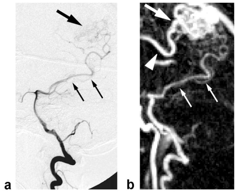
(a) X-ray DSA and (b) MRA of a Spetzler-Martin Grade II right posterior AVM at the same scale and orientation. X-ray DSA spatial resolution: 0.1 × 0.1 mm, temporal resolution: 0.33 sec. MRA pixel size: 1.1 × 1.1 × 2.9 mm, temporal resolution: 5.0 sec, frame rate: 0.5 sec, MIP along the z direction. Smaller arrows denote the feeding artery to the nidus of the AVM. Larger arrows denote the nidus. The MRA demonstrates an additional feeding vessel (arrowhead) not shown on the x-ray due to the selective catheter injection.
DISCUSSION
Despite all the valuable recent research activity in under-sampling, techniques to better sample k-t space for angiography are ultimately limited by SNR and still may be unable to achieve the temporal Nyquist frequency in certain situations. Temporal Nyquist frequency here refers to the minimum temporal resolution necessary to capture all relevant physiological information. For example, attempting to identify an intracranial AVM’s feeding and draining vessels currently pushes 3D CE-MRA to the limit of achievable temporal resolution (23,24). However, even if the true temporal resolution is not substantially increased, there is no reason why the frame rate cannot be increased to the point where frames viewed consecutively in cine mode appear seamless at physiologic frame rates. The sliding window technique generates such intermediate time frames which are useful, for example, when the peak arterial phase occurs between two acquired phases or when assessing whether a potential arteriovenous shunt causes the venous circulation to enhance slightly prematurely. Since MRI data are acquired serially, intermediate time frames may be better centered around the time of a clinically significant event and, therefore, better depict this event. The SNR of a longer acquisition is maintained, though, since SNR is proportional to the square root of imaging time. As an alternative explanation, the temporal resolution of the technique said to be 3.5 sec, but that does not imply the entirety of k-space is instantaneously sampled every 3.5 sec; rather, a new line is acquired for every TR, or 3 ms, and a complete set of new lines is acquired every 3.5 sec. Thus, the sliding window technique takes advantage of the additional information afforded by serial sampling. Another major advantage of the technique relates to the fact that data contributing to a frame only extend over a duration equal to the temporal resolution. Other techniques, such as those based on keyhole, may claim high temporal resolutions, but data are spread widely in time, resulting in artifact. By maintaining such a minimal “temporal aperture,” angiography better approximates true anatomy and physiology.
Undersampling techniques that do actually increase the true temporal resolution may even be used in conjunction with sliding window. For instance, asymmetric sampling and angular undersampling of the radial trajectory provided 3.6× acceleration to the imaging protocol in this study. However, asymmetric sampling degrades spatial resolution, hence the use of “pixel size” rather than “spatial resolution” in listing scan parameters. Also, angular undersampling primarily degrades SNR (not spatial resolution as much for moderate angular undersampling factors since the streak artifact is displaced from its source, and artifact can simply be considered spatially correlated noise). When choosing an acceleration method, it may be preferable to combine different techniques, each with low acceleration, to achieve an overall high acceleration rather that rely on a single technique (16,24). The artifact associated with each technique will not necessarily combine coherently, and therefore the overall artifact may appear less severe.
In this way the rationale for the CE-MRA technique starts with the use of sliding window reconstruction plus acceleration methods. Next, it is logical to consider how to best order samples considering that k-space must be traversed along a continuous path, or trajectory. The first general design criterion for ordering samples is that the central region of k-space should be sampled more frequently than the peripheral region because the central region is known to have a higher temporal Nyquist frequency, and it contains substantially more image energy. The radial trajectory achieves this goal by sampling the center of k-space with higher density. Spiral trajectories and the VIPR trajectory (25) also can sample the center with higher density, but the spin-warp trajectory cannot. It has yet to be proven which of these trajectories results in the best combination of SNR, spatial resolution, and temporal resolution for 4D CE-MRA. Acceleration methods such as parallel imaging and TRICKS have different temporal sampling rates for central and peripheral segments, but the boundary between these segments produces a discontinuity in the temporal sampling rate, and the boundary’s location may be considered arbitrary. In summary, one way of increasing temporal resolution is to choose the sampling method that best matches the spatial frequency-dependent temporal Nyquist frequency of the particular application.
The second general design criterion for ordering samples involves the fact that samples exhibit more correlation with those in their neighborhood than elsewhere in k-space. Thus, samples distributed in k-t space will be minimally correlated and better capture dynamic information. The pseudorandom ordering method attempts to distribute samples both within a frame/segment and from frame to frame. The problem of how to order views has been studied extensively in a general sense and for other applications (26–28); however, the approach to ordering described here is specifically for 4D CE-MRA. Ordering techniques previously developed for angiography are based on other sampling patterns (18,29).
With high frame rates, the applications for 4D CE-MRA expand into areas traditionally occupied by x-ray DSA. The short bolus length and rapid contrast wash-out of x-ray DSA as a result of local, selective contrast injection are what motivated the sliding subtraction technique. While clinicians may be more accustomed to the contrast bolus behaving in this manner, the sliding subtraction technique has additional advantages. Since the time between the two volumes involved in the subtraction operation, the lag time, is less than that for conventional subtraction, there is less possibility of patient motion corrupting the data, especially toward the end of the scan. Most importantly, though, with conventional subtraction, enhancement persists in vessels and wash-out is gradual due to the fact that significant dispersion of the bolus of contrast agent occurs between the site of injection (typically an antecubital vein) and the vessels of interest. The appearance of rapid wash-out of contrast enables later phases, such as venous phases, to be relatively uncontaminated by portions of vessels enhancing earlier. The signal versus time curves in Fig. 8 demonstrate this separation of arterial and venous enhancement. The ability to precisely time wash-in and wash-out is crucial to the grading of, for example, AVMs, where draining veins will exhibit premature enhancement (30).
The sliding mask subtraction is related to techniques previously described in the context of x-ray DSA (31) and interventional MRI (32). The challenges of 4D CE-MRA, though, call for certain unique implementation details. In particular, the subtraction lag time has an effect on the resulting angiogram’s CNR. At shorter lag times, signal at a given point in a vessel would have less opportunity to change, and therefore the CNR would decrease. The CNR for sliding mask subtraction is inferior for certain choices of lag time, but as long as the lag time is chosen wisely, the CNR can approach or exceed that of initial mask subtraction. Artery-background and vein-background CNR are no longer significantly different from that of the initial mask subtraction technique at a lag time of 15 sec, and artery-vein CNR is superior at lag times of 12.5 sec or longer. Another metric of image quality is the overlap integral, and for all lag times the sliding mask subtraction is superior. Longer lag times result in a decreasing overlap integral up to 10 sec and in an increasing overlap integral over 10 sec. This suggests that the optimal lag time may be at 10 sec. However, other factors also contribute, such as the fact that there is less sensitivity to motion at lower lag times. In addition, a patient’s specific flow dynamics would certainly alter the choice of an optimal lag time.
The patient study demonstrated the clinical application of the proposed technique and provided a useful comparison to x-ray DSA, the gold standard for time-resolved angiography. Despite the superior in-plane spatial resolution and temporal resolution of x-ray DSA, 4D MRA may find utility in clinical situations where the risks associated with nephrotoxic contrast, ionizing radiation, and an endovascular procedure outweigh the benefit of better image quality, not to mention the greater cost and time commitment of diagnostic x-ray angiography.
While the radial trajectory offers the benefit of variable sampling density, certain challenges arise that do not present difficulties for spin-warp imaging. First, the radial trajectory is more sensitive to trajectory/timing errors. For radial imaging, error along the read-out direction manifests itself as spatial blurring. The same error results in an image domain phase shift for spin-warp imaging, which has no effect on generating magnitude images. Timing errors between the three orthogonal gradient fields can be a significant source of error, and a correction technique has been proposed (33). Second, combining radial and parallel imaging is challenging. Although any non-Cartesian sampling can be used with parallel imaging, only Cartesian sampling is computationally efficient (34). Parallel imaging can be applied in the through-plane dimension for cylindrical sampling patterns, but the imaging slab must be thick enough to allow sufficient variation in coil sensitivities in the through-plane dimension for proper reconstruction. Currently, non-Cartesian parallel imaging is an active area of research in the field (35).
A limitation of this study was the fact that flow dynamics may change from person to person and, therefore, pooling or comparing data from different volunteers is not entirely valid. Despite this variability, reasonable statistical conclusions could still be reached. Another limitation was the use of asymmetric sampling/zero-filled reconstruction. A true partial Fourier reconstruction with estimation of the phase map from low-frequency data may provide superior image quality. On a related note, the linear density compensation function did not make any correction for sampling density due to asymmetric sampling, which likely leads to reduced spatial resolution. Development of this technique at higher field has the potential for higher SNR (ultimately to be converted to higher temporal resolution), but, among other challenges, trajectory errors could theoretically become more pronounced with worse B0 inhomogeneity due to increased susceptibility. Image quality of the patient study at 3T appeared comparable to that of the volunteer studies at 1.5T, so high field development seems promising. The intracranial circulation was chosen in this study because its short arteriovenous transit time (3–4 sec) necessitates fast imaging and there are potential clinical applications to such pathologies as intracranial arteriovenous fistulae and malformations. Other anatomic regions may also benefit from this technique.
CONCLUSIONS
With the goal of imaging blood flow dynamics with 4D angiography, several components of the conventional CE-MRA procedure were reexamined to accommodate the demand for high temporal resolution and cine visualization. The result was a method capable of producing image matrices of 192 × 192 × 27 at ≈ 3 frames/sec. Specifically, k-space sampling was performed with 3D cylindrical sampling and pseudorandom view ordering, undersampling enabled increased temporal resolution, reconstruction relied on a sliding window to interpolate time frames to cine frame rates, and a sliding subtraction technique provided statistically significant improvement in separation of artery/vein enhancement in time.
Acknowledgments
The authors thank Nondas Leloudas and Sharon Coffey for help with volunteer studies.
References
- 1.Prince MR, Yucel EK, Kaufman JA, Harrison DC, Geller SC. Dynamic gadolinium-enhanced three-dimensional abdominal MR arteriography. J Magn Reson Imaging. 1993;3:877–881. doi: 10.1002/jmri.1880030614. [DOI] [PubMed] [Google Scholar]
- 2.Crummy AB, Stieghorst MF, Turski PA, Strother CM, Lieberman RP, Sackett JF, Turnipseed WD, Detmer DE, Mistretta CA. Digital subtraction angiography: current status and use of intra-arterial injection. Radiology. 1982;145:303–307. doi: 10.1148/radiology.145.2.6753013. [DOI] [PubMed] [Google Scholar]
- 3.Riederer SJ, Tasciyan T, Farzaneh F, Lee JN, Wright RC, Herfkens RJ. MR fluoroscopy: technical feasibility. Magn Reson Med. 1988;8:1–15. doi: 10.1002/mrm.1910080102. [DOI] [PubMed] [Google Scholar]
- 4.Zhu H, Buck DG, Zhang Z, Zhang H, Wang P, Stenger VA, Prince MR, Wang Y. High temporal and spatial resolution 4D MRA using spiral data sampling and sliding window reconstruction. Magn Reson Med. 2004;52:14–18. doi: 10.1002/mrm.20167. [DOI] [PubMed] [Google Scholar]
- 5.van Vaals JJ, Brummer ME, Dixon WT, Tuithof HH, Engels H, Nelson RC, Gerety BM, Chezmar JL, den Boer JA. “Keyhole” method for accelerating imaging of contrast agent uptake. J Magn Reson Imaging. 1993;3:671–675. doi: 10.1002/jmri.1880030419. [DOI] [PubMed] [Google Scholar]
- 6.Doyle M, Walsh EG, Blackwell GG, Pohost GM. Block regional interpolation scheme for k-space (BRISK): a rapid cardiac imaging technique. Magn Reson Med. 1995;33:163–170. doi: 10.1002/mrm.1910330204. [DOI] [PubMed] [Google Scholar]
- 7.Korosec FR, Frayne R, Grist TM, Mistretta CA. Time-resolved contrast-enhanced 3D MR angiography. Magn Reson Med. 1996;36:345–351. doi: 10.1002/mrm.1910360304. [DOI] [PubMed] [Google Scholar]
- 8.Krishnan S, Chenevert TL. Spatio-temporal bandwidth-based acquisition for dynamic contrast-enhanced magnetic resonance imaging. J Magn Reson Imaging. 2004;20:129–137. doi: 10.1002/jmri.20090. [DOI] [PubMed] [Google Scholar]
- 9.Sodickson DK, Manning WJ. Simultaneous acquisition of spatial harmonics (SMASH): fast imaging with radiofrequency coil arrays. Magn Reson Med. 1997;38:591–603. doi: 10.1002/mrm.1910380414. [DOI] [PubMed] [Google Scholar]
- 10.Griswold MA, Jakob PM, Heidemann RM, Nittka M, Jellus V, Wang J, Kiefer B, Haase A. Generalized autocalibrating partially parallel acquisitions (GRAPPA) Magn Reson Med. 2002;47:1202–1210. doi: 10.1002/mrm.10171. [DOI] [PubMed] [Google Scholar]
- 11.Pruessmann KP, Weiger M, Scheidegger MB, Boesiger P. SENSE: sensitivity encoding for fast MRI. Magn Reson Med. 1999;42:952–962. [PubMed] [Google Scholar]
- 12.Scheffler K, Hennig J. Reduced circular field-of-view imaging. Magn Reson Med. 1998;40:474–480. doi: 10.1002/mrm.1910400319. [DOI] [PubMed] [Google Scholar]
- 13.Peters DC, Korosec FR, Grist TM, Block WF, Holden JE, Vigen KK, Mistretta CA. Undersampled projection reconstruction applied to MR angiography. Magn Reson Med. 2000;43:91–101. doi: 10.1002/(sici)1522-2594(200001)43:1<91::aid-mrm11>3.0.co;2-4. [DOI] [PubMed] [Google Scholar]
- 14.Vigen KK, Peters DC, Grist TM, Block WF, Mistretta CA. Undersampled projection-reconstruction imaging for time-resolved contrast-enhanced imaging. Magn Reson Med. 2000;43:170–176. doi: 10.1002/(sici)1522-2594(200002)43:2<170::aid-mrm2>3.0.co;2-p. [DOI] [PubMed] [Google Scholar]
- 15.Tsao J, Boesiger P, Pruessmann KP. k-t BLAST and k-t SENSE: dynamic MRI with high frame rate exploiting spatiotemporal correlations. Magn Reson Med. 2003;50:1031–1042. doi: 10.1002/mrm.10611. [DOI] [PubMed] [Google Scholar]
- 16.Kellman P, Epstein FH, McVeigh ER. Adaptive sensitivity encoding incorporating temporal filtering (TSENSE) Magn Reson Med. 2001;45:846–852. doi: 10.1002/mrm.1113. [DOI] [PubMed] [Google Scholar]
- 17.Maki JH, Prince MR, Londy FJ, Chenevert TL. The effects of time varying intravascular signal intensity and k-space acquisition order on three-dimensional MR angiography image quality. J Magn Reson Imaging. 1996;6:642–651. doi: 10.1002/jmri.1880060413. [DOI] [PubMed] [Google Scholar]
- 18.Wilman AH, Riederer SJ. Performance of an elliptical centric view order for signal enhancement and motion artifact suppression in breath-hold three-dimensional gradient echo imaging. Magn Reson Med. 1997;38:793–802. doi: 10.1002/mrm.1910380516. [DOI] [PubMed] [Google Scholar]
- 19.Haase A, Matthaei D, Hanicke W, Frahm J. Dynamic digital subtraction imaging using fast low-angle shot MR movie sequence. Radiology. 1986;160:537–541. doi: 10.1148/radiology.160.2.3523597. [DOI] [PubMed] [Google Scholar]
- 20.Rasche V, de Boer RW, Holz D, Proksa R. Continuous radial data acquisition for dynamic MRI. Magn Reson Med. 1995;34:754–761. doi: 10.1002/mrm.1910340515. [DOI] [PubMed] [Google Scholar]
- 21.Shankaranarayanan A, Simonetti OP, Laub G, Lewin JS, Duerk JL. Segmented k-space and real-time cardiac cine MR imaging with radial trajectories. Radiology. 2001;221:827–836. doi: 10.1148/radiol.2213010455. [DOI] [PubMed] [Google Scholar]
- 22.Jackson JI, Meyer CH, Nishimura DG, Macovski A. Selection of a convolution function for Fourier inversion using gridding. IEEE Trans Med Imaging. 1991;10:473–478. doi: 10.1109/42.97598. [DOI] [PubMed] [Google Scholar]
- 23.Ziyeh S, Strecker R, Berlis A, Weber J, Klisch J, Mader I. Dynamic 3D MR angiography of intra- and extracranial vascular malformations at 3T: a technical note. AJNR Am J Neuroradiol. 2005;26:630–634. [PMC free article] [PubMed] [Google Scholar]
- 24.Cashen TA, Carr JC, Shin W, Walker MT, Futterer SF, Shaibani A, McCarthy RM, Carroll TJ. Intracranial time-resolved contrast-enhanced MR angiography at 3T. AJNR Am J Neuroradiol. 2006;27:822–829. [PMC free article] [PubMed] [Google Scholar]
- 25.Barger AV, Block WF, Toropov Y, Grist TM, Mistretta CA. Time-resolved contrast-enhanced imaging with isotropic resolution and broad coverage using an undersampled 3D projection trajectory. Magn Reson Med. 2002;48:297–305. doi: 10.1002/mrm.10212. [DOI] [PubMed] [Google Scholar]
- 26.Theilmann RJ, Gmitro AF, Altbach MI, Trouard TP. View-ordering in radial fast spin-echo imaging. Magn Reson Med. 2004;51:768–774. doi: 10.1002/mrm.20031. [DOI] [PubMed] [Google Scholar]
- 27.Welch EB, Rossman PJ, Felmlee JP, Manduca A. Self-navigated motion correction using moments of spatial projections in radial MRI. Magn Reson Med. 2004;52:337–345. doi: 10.1002/mrm.20151. [DOI] [PubMed] [Google Scholar]
- 28.Tsao J, Boesiger P, Pruessmann KP. Lattice permutation for reducing motion artifacts in radial and spiral dynamic imaging. Magn Reson Med. 2006;55:116–125. doi: 10.1002/mrm.20743. [DOI] [PubMed] [Google Scholar]
- 29.Pipe JG, Ahunbay E, Menon P. Effects of interleaf order for spiral MRI of dynamic processes. Magn Reson Med. 1999;41:417–422. doi: 10.1002/(sici)1522-2594(199902)41:2<417::aid-mrm29>3.0.co;2-w. [DOI] [PubMed] [Google Scholar]
- 30.Spetzler RF, Martin NA. A proposed grading system for arteriovenous malformations. J Neurosurg. 1986;65:476–483. doi: 10.3171/jns.1986.65.4.0476. [DOI] [PubMed] [Google Scholar]
- 31.Kruger RA, Mistretta CA, Riederer SJ. Physical and technical considerations of computerized fluoroscopy difference imaging. IEEE Trans Nucl Sci. 1981;28:205–212. [Google Scholar]
- 32.Bakker CJ, Seppenwoolde JH, Bartels LW, van der Weide R. Adaptive subtraction as an aid in MR-guided placement of catheters and guide-wires. J Magn Reson Imaging. 2004;20:470–474. doi: 10.1002/jmri.20126. [DOI] [PubMed] [Google Scholar]
- 33.Peters DC, Derbyshire JA, McVeigh ER. Centering the projection reconstruction trajectory: reducing gradient delay errors. Magn Reson Med. 2003;50:1–6. doi: 10.1002/mrm.10501. [DOI] [PMC free article] [PubMed] [Google Scholar]
- 34.Pruessmann KP, Weiger M, Bornert P, Boesiger P. Advances in sensitivity encoding with arbitrary k-space trajectories. Magn Reson Med. 2001;46:638–651. doi: 10.1002/mrm.1241. [DOI] [PubMed] [Google Scholar]
- 35.Samsonov AA, Block WF, Arunachalam A, Field AS. Advances in locally constrained k-space-based parallel MRI. Magn Reson Med. 2006;55:431–438. doi: 10.1002/mrm.20757. [DOI] [PubMed] [Google Scholar]