

Abstract
In the present study, the cascaded interactions between stimuli and neural and hemodynamic responses were modeled using linear systems. These models provided the theoretical hypotheses that were tested against the electroencephalography (EEG) and blood oxygen level dependent (BOLD) functional magnetic resonance imaging (fMRI) data recorded from human subjects during prolonged periods of repeated visual stimuli with a variable setting of the inter-stimulus-interval (ISI) and visual contrast. Our results suggest that 1) neural response is nonlinear only when ISI<0.2 s, 2) BOLD response is nonlinear with an exclusively vascular origin when 0.25<ISI<4.2 s, 3) vascular response nonlinearity reflects a refractory effect, rather than a ceiling effect, and 4) there is a strong linear relationship between the BOLD effect size and the integrated power of event-related synaptic current activity, after modeling and taking into account the vascular refractory effect. These conclusions offer important insights into the origins of BOLD nonlinearity and the nature of neurovascular coupling, and suggest an effective means to quantitatively interpret the BOLD signal in terms of neural activity. The validated cross-modal relationship between fMRI and EEG may provide a theoretical basis for the integration of these two modalities.
Keywords: Neurovascular Coupling, BOLD Nonlinearity, BOLD-fMRI Modeling, Visual Evoked Potential, Refractory Effect
Introduction
Functional magnetic resonance imaging (fMRI) typically uses the BOLD signal to infer neural activity (Bandettini et al., 1992; Kwong et al., 1992; Ogawa et al., 1992). Most fMRI studies assume that the temporal behavior of the BOLD signal in an activated voxel is predictable by convolving the stimuli with a linear time-invariant system (Cohen, 1997; Dale and Buckner, 1997; Friston et al., 1994). Although this assumption has proven useful and efficient in functional neuroimaging, its validity is challenged by studies in which the stimuli-to-BOLD relationship has been found to be nonlinear to various degrees (Birn and Bandettini, 2005; Boynton et al., 1996; Huettel and McCarthy, 2000; Vazquez and Noll, 1998; Zhang et al., 2008b; de Zwart et al., 2009). What remains unclear is the origin of BOLD nonlinearity. It may arise from a nonlinear neural response to stimuli and/or a nonlinear vascular/metabolic response to neural activity (Birn and Bandettini, 2005). While the former is often attributed to neural refractory (Budd et al., 1998) and adaptation (Muller et al., 1999) effects, the latter points to the composite nature of the BOLD contrast, which depends on a complex interplay between cerebral blood flow, blood volume, and oxygen consumption in response to neural activation (Buxton et al., 2004).
The quantitative coupling between neural and hemodynamic signals remains a topic of debate. Previous studies on humans or animal models have arrived at differing conclusions in support of the linearity (Arthurs et al. 2000; Herman et al., 2009; Huttunen et al., 2008; Lauritzen, 2001; Logothetis et al., 2001; Martindale et al., 2003; Nangini et al., 2008; Ou et al., 2009) or nonlinearity (Devor et al., 2003; Hewson-Stoate et al., 2005; Hoffmeyer et al., 2007; Sheth et al., 2004; de Zwart et al., 2009) of neurovascular coupling. Most of these studies share a common strategy: graded sensory (or neural) stimulation is employed to elicit changes in both electrophysiological and hemodynamic signals, which are recorded and quantified individually before being compared against a linear or nonlinear function. Existing disagreements on the linearity of neurovascular coupling may be accounted for in part by the variance in signal quantification methods used across studies. A pair of quantitative measures of multimodal signals needs to be consistent from physical, physiological, and system perspectives in order to correctly assess the cross-modal relationship. The use of inconsistent quantities could lead to misleading conclusions that are difficult to compare across studies.
In the present study, we modeled the cascaded interactions between stimuli and neural and hemodynamic responses using linear systems (or their variations), as illustrated in Fig. 1.A (or Fig. 1.B). These mathematical models provided the theoretical hypotheses that were tested against the EEG and BOLD-fMRI data recorded from human subjects during sustained and repeated visual stimulation. By varying the stimulus frequency and contrast, the linearity/nonlinearity of the EEG and fMRI responses was evaluated in an attempt to pinpoint the neural and vascular origins of BOLD nonlinearity. The linearity of neurovascular coupling was further investigated by assessing the relationship between a pair of metrics rigorously derived from the system models and used to quantify the measured neural and hemodynamic responses.
Fig. 1.
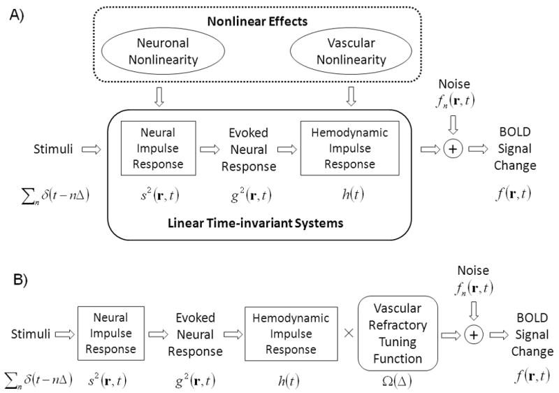
A) Diagram of the linear system models. Repeated stimuli are modeled as a train of delta functions, Σnδ(t-nΔ). Neural impulse response function represents the synaptic current activity, s(r,t), specific to a location r within the brain, induced by a single stimulus. s2(r,t) represents the power of the neural impulse response. If neural response is linear, the steady-state neural response evoked by the repeated stimuli, denoted as g(r,t), can be derived from the stimuli as g(r,t)=Σnδ(t- nΔ)*s(r,t). If neural and hemodynamic responses are coupled in a linear manner, the BOLD response can be represented by convolving the power (or magnitude) of the evoked neural response, g2(r,t), with the hemodynamic impulse response function, h(t), plus noise fn(r,t). See Equations (1) through (5) in the text. These relationships rely on the assumptions of two linear time-invariant systems, which may be affected by the possible nonlinearities in both neural and vascular responses. B) Diagram of the system models after adding a nonlinear component, in terms of the ISI, to the linear system illustrated in A). This nonlinear component corrects the vascular refractory effect (see the Results section for more details).
Materials and Methods
Linear System Modeling
If the linearity holds true for both the neural and hemodynamic responses to a sustained period of repeated stimuli separated in time by an inter-stimulus-interval (ISI) (also denoted as Δ), the BOLD-fMRI signal change can be expressed as a linear function of the stimuli. As illustrated in Fig. 1.A, this linear relationship can be mathematically described as a two-step convolution model.
| (1) |
In the above model, f(r,t) and fn(r,t) stand for the measured hemodynamic signal and noise, respectively, at a brain location r and time t. Σnδ(t − nΔ) represents a train of delta functions separated by an interval Δ. Such a delta-function train is used to model the repetitive and discrete “events”, whose time of occurrence is typically the stimulus onset (or offset) time even though the stimulus itself is not transient. s2(r,t) stands for the power of the “event-related” (or impulse) neural response, which specifically represents the post-synaptic current response following a single stimulus. h(t) stands for the hemodynamic impulse response function (HRF).
By defining a temporal regressor, p(t), as in Eq. (2), a linear regression model (Eq. (3)) can be derived from Eq. (1).
| (2) |
| (3) |
Note that the above derivation is based on the fact that the hemodynamic signal keeps approximately unchanged during the relatively short time span of the event-related neural response, denoted as T.
Importantly, the regression model, as expressed by Eq. (3), implies a linear relationship between the BOLD effect size, denoted as β(r), and the integrated power of the neural impulse response (Liu and He, 2008). As shown in Eq. (4), an estimate of the BOLD effect size, denoted as β̂(r), can be obtained by computing the “optimal” ratio between the measured BOLD-fMRI signal and the regressor using Eq. (4).
| (4) |
Similarly, if the BOLD response is coupled with the magnitude, instead of the power, of synaptic current, a linear relationship can be derived as in Eq. (5)
| (5) |
Eq. (4) and Eq. (5) point to the same way of quantifying the BOLD signal in response to a block of multiple stimuli. But the interpretation of the quantified BOLD effect size is differently expressed in terms of the corresponding neural response to a single stimulus.
Subjects
Fifteen healthy human subjects (age 23±4, 6 female) were studied after giving informed written consent in accordance with a protocol approved by the institutional review board at the University of Minnesota. All subjects had normal or corrected-to-normal vision. Subjects participated in all or part of the following experiments.
Experiments
Paradigm 1 for Studying Neural Response Nonlinearity
Scalp EEG signals were recorded from five subjects presented with sustained full-screen pattern-reversal checkerboard stimuli (10×10 black-and-white squares) with a variable ISI. The ISI was first set as 2000 ms, and the reversal stimuli were repeated for about 1000 times. Nine distinct ISI values were then pseudo-randomly selected from 40 to 533 ms over subsequent runs. The order of runs was also randomized. In each run, the stimuli were presented for a sustained period of ≥40 s to allow the evoked neural response to reach the steady state. The stimuli with a longer ISI were presented for a period of time, so that the total number of stimulus presentations was comparable across runs. The stimuli were presented with a fixation cross at the center of a liquid crystal display (LCD) flat-panel monitor placed inside a dark shielding room.
Paradigm 2 for Studying Hemodynamic Response Nonlinearity
BOLD-fMRI signals were recorded from ten subjects presented with sustained quarter-circular grating visual stimuli in the lower-right quadrant of the visual field. The experiment consisted of two sessions. The stimulus contrast was set as 100% (black vs. white) in one session and as 10% (dark vs. light gray) in the other session. Each fMRI session consisted of multiple 30-s stimulus blocks interleaved with 30-s control blocks (a central fixation point on a neutral gray background). A distinct ISI value, ranging from 250 to 6000 ms, was applied to each stimulus block. The stimuli were projected through a digital light processing (DLP) projector to a screen inside the MRI scanner, and back mirrored through a 45-degree mirror placed above the subjects' forehead.
Paradigm 3 for Studying fMRI-EEG Coupling
Both fMRI and EEG signals were recorded from ten subjects presented with a lower-right quarter-circular grating visual pattern reversing at an ISI of 500 ms with a variable contrast (5, 10, 20, 40, 60, 80 and 100%). In each experiment, seven 30-s blocks with sustained stimuli of varying contrast were interleaved with eight 30-s control blocks. The experiment was repeated at least four times for each subject. The EEG and fMRI signals were acquired simultaneously from five subjects and separately from the other five subjects. The setting for the stimulus presentation was identical to Paradigm 2.
MRI/fMRI Data Acquisition
The MRI and fMRI measurements were obtained in a 3-T/90-cm bore magnet (Siemens Trio, Siemens, Germany) equipped with an eight-channel phase array head volume coil. For each subject, the whole-head anatomy was first acquired sagittally using a 3D MPRAGE sequence (matrix size: 256×256×240; spatial resolution: 1×1×1 mm3; TR/TE = 20/5 ms). The BOLD-fMRI data was acquired with 18 axial T2*-weighted images covering both the occipital and parietal lobes using a gradient-echo echo-planar imaging (EPI) sequence (matrix size: 64×64; in-plane resolution: 3×3 mm2; slice thickness: 3 mm; no gap between slices; TR/TE = 1000/35 ms).
EEG Recordings
When acquiring EEG alone, a Neuroscan SynAmps2 system (Compumedics, Charlotte, USA) was used to continuously record scalp potentials from 64 electrodes placed according to the extended international 10/20 system. The data were referenced to FCz, sampled at 1000 Hz, and band-pass filtered from 0.3 to 70 Hz. A pair of bipolar electrodes was placed above and below the left eye to monitor eye blinks.
When acquiring EEG and fMRI simultaneously, a BrainAmp MR Plus system (BrainProducts, Munich, Germany) was used to record EEG from 64 scalp electrodes. The data were referenced to FCz, sampled at 5000 Hz, and low-pass filtered (≤250 Hz) using two MR-compatible amplifiers placed inside the magnet. A unipolar electrode was placed above the left eye to monitor eye blinks. An additional electrode was placed on the back of the subject to record electrocardiograms (ECG). The digitized EEG/ECG signals were transmitted via optical fibers to a recording computer in the control room. The onsets of EPI volume acquisitions were marked in EEG recordings using a trigger signal sent from the MRI scanner to the recording computer. Prior to recording, the locations of all electrodes and three landmark points (nasion, preauricular left, preauricular right) were determined by a radiofrequency localizer (Polhemus Fastrak, VT, USA).
fMRI Data Analysis
The fMRI data was processed using BrainVoyager QX (Brain Innovation, Maastricht, Netherlands). Several preprocessing steps were applied to the raw EPI volumes, including head motion correction, slice scan time correction, linear trend removal and high-pass filtering (3 cycles per scanning session). The preprocessed fMRI data were co-registered with the subjects' anatomical images.
For each individual subject, the fMRI data were analyzed by using a modified general linear model (GLM) (Liu and He, 2008). As mathematically described in Eq. (2), rather than using a conventional “box-car” function, we represented each regressor in the design matrix by convolving a train of delta functions (indexing the occurrences of discrete visual stimuli) with a canonical HRF. By fitting the model (Eq. (3)) with the fMRI data, we estimated the BOLD effect size as the regression coefficient (see Eq. (4)). A statistical parametric map contrasting the stimulus conditions vs. the control condition was obtained by illustrating the corresponding t-statistics with a p<0.01 threshold after the Bonferroni correction. From this map, five regions of interest (ROI) were defined to cover one striate area within the left primary visual cortex, or V1 (contralateral to the stimulus location), and two symmetric pairs of extra-striate areas. The time courses of the BOLD percentage change were first averaged within each ROI and then averaged across subjects. For the ROI-level analysis, the BOLD time course within the V1 ROI was fitted with the aforementioned GLM, resulting in a value of the BOLD effect size for each distinct combination of visual contrast and ISI. For the group-level analysis, individual subjects' fMRI data were re-aligned to a common Talairach space and analyzed using a multi-study GLM implemented in BrainVoyager QX (Goebel et al., 2006).
EEG Data Analysis
The EEG data acquired simultaneously with fMRI were first corrected by removing MR gradient artifacts and cardiac ballistic artifacts using template subtraction methods (Allen et al., 1998, 2000) implemented in BrainVision Analyzer (BrainProducts, Munich, Germany). The corrected EEG data or the EEG signals recorded without concurrent fMRI were visually inspected to identify and thereby reject periods of eye-blink artifacts. For visual stimuli with ISI=2000 ms (for Paradigm 1) and ISI=500 ms (for Paradigm 3), the EEG signals were segmented into about 1000 single-trial epochs from -100 to 500 ms around stimulus onsets. Linear de-trend and pre-stimulus baseline correction were sequentially applied to the segmented epochs before averaging the signals across epochs to obtain the event-related potentials (ERP), also referred to as visual evoked potentials (VEP) in this paper.
For Paradigm 1, the steady-state visual evoked potentials (SSVEP) measured during sustained and repeated stimuli with ISIs between 40 and 533 ms, were quantitatively compared with a linear prediction of the SSVEP, derived by convolving the stimulus function with the VEP obtained when ISI=2000 ms. Both the measured and predicted SSVEP signals were transformed to the frequency domain via the fast Fourier transformation (FFT) implemented in Matlab (Mathworks, Natick, USA). The amplitudes at the stimulus frequency and its harmonic frequencies (up to 40 Hz), inversely weighted by the corresponding amplitudes in the stimulus spectrum, were summed individually for the measured and predicted SSVEP spectra. The ratio between them, referred to as the recovery coefficient (RCC), was computed for each ISI. If neural response linearity holds true, the RCC value should be close to one. Alternatively, an RCC value smaller than one suggests a neural refractory effect, and an RCC value larger than one suggests a facilitative effect. See the Appendix for mathematical details about the spectral analysis employed in this study.
For Paradigm 3, electrical source activities at V1 and the other extra-striate areas were estimated by using BESA (MEGIS, Graefeling, Germany) to fit five fixed current dipoles to the VEP signals generated by visual stimuli with ISI=500 ms and variable contrasts (5%∼100%). The ROIs defined from the fMRI activation map were used to seed the dipole locations in BESA (Vanni et al., 2004; Di Russo et al., 2005). The seed points were selected as the centers of the mass of the activated fMRI ROIs. The multiple-dipole model was fixed from -100 to 500 ms around the stimulus onset. After the dipole fitting, we summed the power of the estimated V1 dipole moment within a post-stimulus period T, where T ranged from 150 to 500 ms. To exclude the contribution from noise, we then subtracted the average pre-stimulus baseline power multiplied by T. In a similar way, we also computed the integrated magnitude of the V1 dipole.
Results
Neural Response Nonlinearity
If neural response is linear, the SSVEP generated by a sustained period of repeated visual stimuli should be predictable by convolving the stimuli with the VEP obtained in response to a single stimulus (Paradigm 1). At various ISIs, we compared the measured and predicted SSVEP represented in both time and frequency domains. When the ISI was long (e.g. 250 ms), the measured SSVEP signal from a middle occipital electrode (Oz) was pseudo-periodic and phase-locked to the stimuli (Fig. 2.a, blue). In the time domain, this signal was well predicted by convolving the stimuli with the VEP from the same electrode (Fig. 2.a, red). In the frequency domain, both of the predicted and measured SSVEP spectra (Fig. 2.b and Fig. 2.c, respectively) peaked at the multiples of the stimulus frequency. The amplitude maps (Fig.2.c) are spatially consistent across these harmonic frequencies, suggesting a common source region within the primary visual cortex. Comparing the predicted and measured SSVEP spectra, we found that the weighted sums of their peak amplitudes were comparable, resulting in a RCC value close to one. However, when the ISI was short (e.g. around 100 ms), the RCC value was considerably smaller than one, which reflects a nonlinear refractory effect.
Fig. 2.
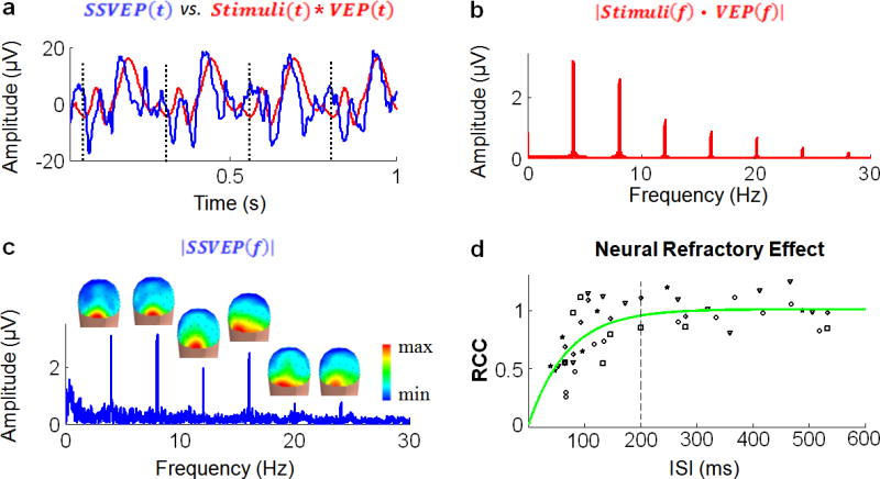
Neural response linearity/nonlinearity. a. Example of a 1-s period of the SSVEP signal measured from Oz is shown in blue. Corresponding linear prediction, derived by convolving the stimuli with the VEP signal at Oz, is shown in red. Vertical dashed lines represent the onsets of 4-Hz visual stimuli. b. Amplitude spectrum of the predicted SSVEP (red curve). c. Amplitude spectrum of the SSVEP measured from Oz (blue curve). Spatial distribution of the SSVEP amplitudes at the stimulus frequency (4 Hz) and its harmonic frequencies (8, 12, 16, 20, 24 Hz) are shown as 3-D scalp maps. d. Scatter-plot of the RCC values obtained from individual subjects at various ISIs (displayed as different symbols). An exponential function fitting the RCC-ISI values is illustrated by a curve in green. Vertical dashed line represents a neural refractory period of 200 ms. As such, neural response to repeated stimuli with ISI>200 ms is approximately linear (0.95<RCC≤1.01). When ISI<200 ms, the steady-state neural response is nonlinear (RCC<0.95). The shorter the ISI, the larger the degree of neural response nonlinearity.
Fig. 2.d plots the RCC values at various ISIs. A neural refractory effect (i.e. RCC<1) was observed mainly when ISI<200 ms, whereas the neural response was approximately linear (i.e. RCC≈1) for longer ISIs. This neural refractory effect was further modeled by an exponential function, denoted as Γ(Δ), which best fitted the RCC-ISI values illustrated in Fig.2.d.
| (6) |
The limit value of 1.01 suggests that the steady-state neural response is indeed linear when adjacent stimuli are well apart in time. Based on this function, we infer that neural response nonlinearity is ignorable when ISI>194 ms (RCC>0.95).
These results also support a notion that the refractoriness of neural system is not an all-or-none effect governed by a single threshold value for the refractory period. Instead, the degree of neural refractory effect is progressively varied by the interval between evoked neural events. For the primary visual cortex studied here, such a gradual refractory effect appears to be well represented by an exponential function, as Eq. (6), with a time constant of 69 ms.
Vascular Response Nonlinearity
We further tested the linearity of the BOLD-fMRI response to sustained (30-s) visual stimuli with ISIs between 0.25 and 6 s (Paradigm 2). For this range of ISIs, because the neural response is linear (as demonstrated above), a nonlinear BOLD response, if observed, must be exclusively due to a nonlinear vascular response to neural activity (i.e. nonlinear neurovascular coupling).
At a ROI within V1 (Fig.3.a), the BOLD responses to visual stimuli with different ISIs were compared with the corresponding linear regressors derived by convolving the stimuli with the standard HRF. Assuming a linear neurovascular coupling, we can predict monotonically decreasing BOLD responses to the stimulus blocks with increasing ISIs (Fig. 3.b, red). The measured BOLD responses showed a similar trend (Fig. 3.b, blue). However, the predictions decreased more dramatically than the measured signals as the ISI increased. We normalized the steady-state amplitudes of both the measured and predicted BOLD signals by their respective amplitudes when ISI=6 s. As shown in Fig. 3.c, the normalized BOLD amplitudes were consistent between the measurements and the linear predictions when ISI≥4 s, whereas considerable over-predictions were found when ISI<4 s. The shorter the ISI, the more dramatic the deviation from linearity in the measured BOLD response.
Fig. 3.
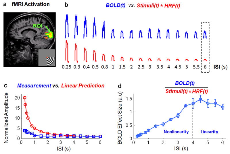
BOLD nonlinearity. a. ROI (surrounded by the green line) selected from the fMRI activation (red-to-yellow) within the upper calcarine sulcus, in response to stimuli presented in the lower-right quadrant of the visual field. b. Group-averaged (n=10) fMRI signals within the ROI shown in a, generated by a 30-s block of stimuli with ISIs from 0.25 to 6 s, are shown in blue. Corresponding regressors, derived by convolving the stimuli with the HRF, are shown in red. c. Steady-state heights of the measured fMRI signals (blue) and the corresponding regressors (red) are plotted as functions of the ISI, after normalizing (to 1) both the measured and modeled steady-state heights when ISI=6 s. d. Ratio between the measured fMRI signal and the regressor (i.e. the BOLD effect size) is plotted as a function of the ISI. Circles represent the group means. Error bars represent the standard errors of the mean (s.e.m) across subjects. The BOLD responses are approximately linear when ISI>4 s (marked by the vertical dashed line). When ISI<4 s, the BOLD responses are nonlinear. The shorter the ISI, the larger the degree of BOLD nonlinearity.
The BOLD effect size, defined as the ratio between the measured BOLD signal (without normalization) and the linear regressor, was computed for each ISI and averaged across subjects. As shown in Fig. 3.d, the BOLD effect size remained approximately constant for ISIs larger than 4 s but became gradually smaller for shorter ISIs. This is in opposition to the theoretical result (Eq. (4)), which suggests a constant BOLD effect size independent of the ISI when both neural and vascular responses can be assumed to be linear (see Eq. (1)). In short, the above results demonstrate the presence of BOLD nonlinearity when 0.25<ISI<4 s, due to nonlinear vascular responses to neural activity.
Vascular Ceiling vs. Refractory Effect
Furthermore, vascular response nonlinearity may be attributed to a vascular refractory effect (Cannestra et al., 1998; Huettel and McCarthy, 2000; Zhang et al., 2008b) or a ceiling effect (Birn and Bandettini, 2005; Bruhn et al., 1994; Buxton et al., 2004). The vascular refractory effect refers to reduced vascular responsiveness when stimulus-evoked neuronal events are too close together in time. The vascular ceiling effect refers to the phenomenon in which a full oxygenation of hemoglobin has been reached so that any increase of neural activity will not lead to a further elevation of the BOLD signal. In contrast to the refractory effect, which depends exclusively on the ISI, the ceiling effect depends on not only the ISI but also the absolute level of the BOLD response to a single stimulus. The smaller the single-stimulus-evoked BOLD response, the shorter the ISI required for repeated stimuli to produce a steady-state BOLD response that reaches the “ceiling”. In other words, one neural event producing a smaller BOLD response has to be repeated more often during a given block period in order to reach the same height as would be reached by less repetitions of the other neural event which produces a relatively stronger BOLD response.
Following this rationale, we reduced the visual contrast from 100% to 10% and repeated the experiment (Paradigm 2), aiming to address whether it was the ceiling effect (or otherwise the refractory effect) that gave rise to the observed BOLD response nonlinearity. The 100% and 10% stimuli were used to produce two types of neural events inducing different levels of BOLD response. Specifically, both the neural and BOLD responses generated by a 10%-contrast visual stimulus were about half as large as those generated by a 100%-contrast stimulus (see Fig. 6).
Fig. 6.
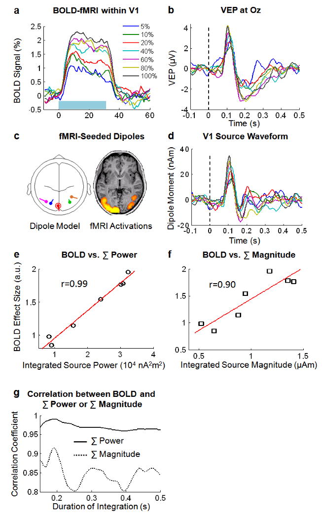
fMRI-EEG coupling. a. BOLD-fMRI signals within V1, induced by a sustained period (30-s, marked by a light blue rectangle) of 2-Hz visual stimuli with seven different contrasts. b. VEP signals at Oz evoked by a single stimulus with variable contrasts. Vertical dashed line represents the stimulus onset. c. fMRI-seeded dipole model. Locations of five dipoles (left) were initiated to the centers of the corresponding ROIs selected from the fMRI activation map (right, p<0.01 corrected). Red-circled dipole represents the dipole in V1. d. Estimated V1 dipole source activity for different contrasts. e & f. Scatter-plot of the BOLD effect sizes within V1 and the integrated power (e) or magnitude (f) of the V1 dipole source, for different visual contrasts. Red lines illustrate linear functions that fit the corresponding scatter points. Data shown in this figure are the average across subjects (n=10). g. Correlations between the BOLD effect size and the integrated source power or magnitude within various post-stimulus periods (0∼150 ms to 0∼500 ms). In a, b and d, visual contrasts are color-coded in a way specified in a.
As demonstrated in Fig. 3.d, the BOLD response generated by 100% stimuli started to deviate from linearity at an ISI of about 4 s. If the vascular response nonlinearity was purely due to the ceiling effect, this means that the BOLD amplitude ceiling would be reached by the response to 100% stimuli repeated every 4 sec within the 30-s block, whereas below this ceiling level the vascular response would be linear. This hypothesis also led us to expect that the 10% stimulus, which produces half of the BOLD response produced by the 100% stimulus, would have to repeat almost twice as fast as the 100% stimuli with a 4-s ISI in order to reach the same amplitude ceiling (see Fig. 4). Therefore, the BOLD nonlinearity would be observed only if ISI≤2 s.
Fig. 4.
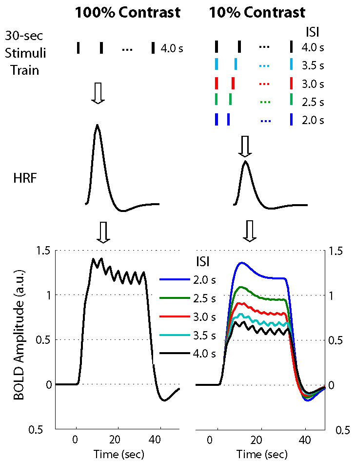
Theoretical comparison between the BOLD-fMRI responses to a 30-s block of 100% (left) and 10% (right) stimuli with various contrasts and ISI, when assuming the BOLD response linearity. These plots are based on the results from computer simulations by assuming the single-stimulus evoked BOLD response amplitude (i.e. the HRF amplitude) for 10% contrast is half as large as that for 100% contrast (as shown in middle). The block BOLD responses (shown in bottom) derived by convolving the stimulus train with variable ISIs (as shown in top) with the respective HRF for both 100% and 10% contrast.
To test this hypothesis, we compared the BOLD effect sizes at various ISIs between the 100% and 10% contrasts. The 10% stimuli produced weaker BOLD signals (and thereby smaller BOLD effect sizes) than the 100% stimuli (Fig. 5.a). Nonlinearity was observed in the BOLD responses to both the 10% and 100% stimuli. This was demonstrated by a BOLD effect size varying across ISIs (Fig. 5.a), as opposed to a constant BOLD effect size as would be observed if the BOLD signal changed proportionately with the linear prediction. Note that the nonlinear trend began at about the same ISI for both of the two stimulus contrasts. This is not likely purely a result of a BOLD ceiling effect, which would hypothetically predict BOLD effect sizes as shown in Fig. 5.b. To better illustrate this point, we normalized the BOLD effect sizes of the measured BOLD signals obtained in response to stimuli with all ISI values by the mean of the “plateau” BOLD effect sizes when ISIs≥4 s. After this normalization, no significant difference was observed between the 10% and 100% contrasts (Fig. 5.c). In a similar way, we also normalized the hypothetically predicted BOLD effect sizes as illustrated in Fig. 5.d. Comparing Fig. 5.c and Fig. 5.d, we found that the observed BOLD nonlinearity was inconsistent with the ceiling effect. The former appeared to be independent of the absolute BOLD response level (variable with the visual contrast), but dependent on the ISI. The above results provide evidence for us to reject the hypothesis that BOLD nonlinearity is due to the vascular ceiling effect, while supporting an alternative source of BOLD nonlinearity – the vascular refractory effect, which depends exclusively on the ISI when neural response is indeed linear.
Fig. 5.
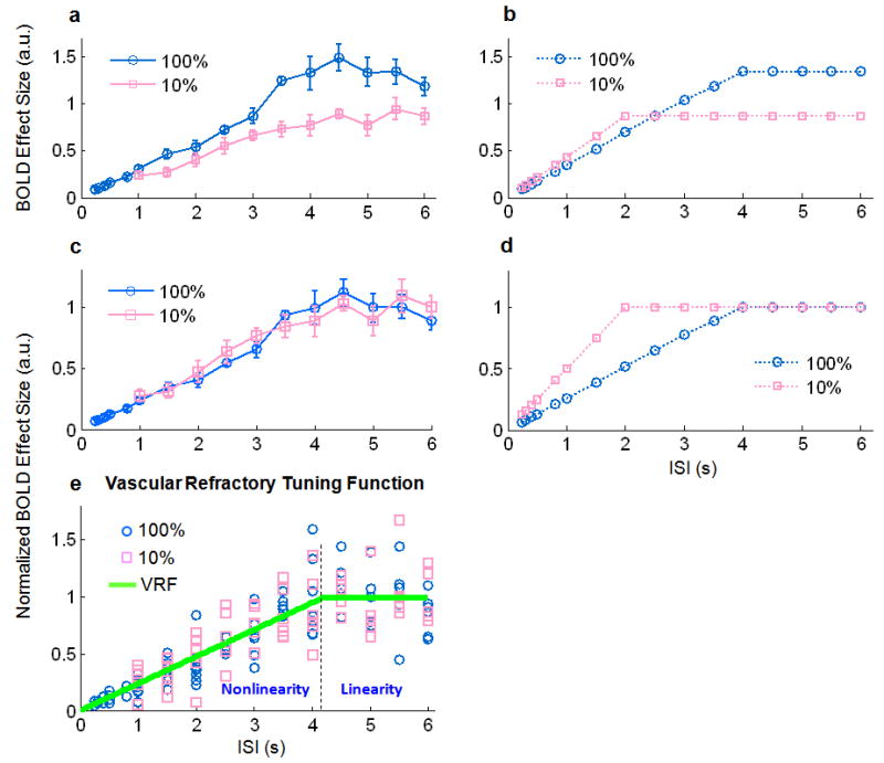
Vascular ceiling vs. refractory effect. a. Group-averaged (n=10) BOLD effect sizes estimated from the measured fMRI signals within V1 in response to stimuli with various ISIs and a 100% (blue) or 10% (pink) visual contrast. b. Theoretical predictions of the BOLD effect sizes at various ISIs in response to 100% or 10% stimuli, by assuming a BOLD ceiling effect. c & d. Curves shown in c and d correspond to the curves shown in a and b, respectively, after normalizing (to 1) the corresponding means of the BOLD effect sizes when ISI≥4 s. e. Scatter-plot of the individual subjects' BOLD effect sizes, normalized in the way described as above, for both the 10% and 100% visual contrasts. A piece-wise linear function fitting all of the points is illustrated by two segments of green lines separated at ISI=4.2 s, which represents the vascular refractory period. Error bars in b and c represent the s.e.m. across subjects.
This vascular refractory effect can be further represented by a vascular refractory tuning function (VRF), denoted as Ω(Δ) in Eq. (7). As shown in Fig. 5.e, this function appears as a piecewise linear curve consisting of two segments of lines: one through the origin and the other as a horizontal line. By best fitting the normalized BOLD effect sizes at various ISIs for every individual subject, the ISI threshold by which the vascular response linearity held true was estimated.
| (7) |
Note that this piecewise linear function is separated at an ISI of 4.2 s, which represents an approximation of the vascular refractory period.
fMRI-ERP Coupling
Importantly, we can refine the linear system models (Eq. (1)), illustrated in Fig. 1, by taking into account the above VRF function to correct the vascular response nonlinearity. When the ISI is longer than neural refractory period, the modified system can be illustrated in Fig. 1.B and mathematically expressed as Eq. (8) with variables defined as aforementioned.
| (8) |
By accordingly modifying the regressor from Eq. (2) to Eq. (9), we can obtain the same linear relationship as described in Eq. (4), meaning that the estimated BOLD effect size should be proportional to the integrated power (or magnitude) of the event-related synaptic current activity.
| (9) |
To test this linear cross-modal relationship, we analyzed the fMRI and VEP responses to 2-Hz visual stimuli with seven different contrasts (Paradigm 3). Fig. 6 summarizes the data and results averaged across 10 subjects. Increasing visual contrasts elevated the BOLD response to a prolonged block of repeated stimuli within V1 (Fig. 6.a), as well as the VEP response to a single stimulus at Oz (Fig. 6.b). By seeding the locations of multiple dipoles to the corresponding fMRI activations (Fig. 6.c), we estimated the dipole moments based on the multi-channel VEP signals. In contrast to the VEP signal at Oz, which was contributed to by activities from both striate and extra-striate regions, the time course of the V1 dipole (Fig. 6.c, red) represented the activity relatively more confined within V1. Comparing Fig. 6.b and Fig. 6.d, we found that the V1 source activity had a shorter duration (about 200 ms) than the VEP signal, suggesting an effective exclusion of the interference from activities occurring within the extra-striate areas during late visual processing. We found a linear relationship (r=0.99) between the BOLD effect size and the integrated V1 source power during a period from 0 to 200 ms following the stimulus onset (Fig. 6.e), in accordance with the theoretical result (Eq. (4)). The integrated V1 source magnitude during the same period was relatively less correlated with the BOLD effect size (r=0.90) (Fig. 6.f). The integrated source power was consistently better correlated than the integrated source magnitude with the BOLD effect size for various durations of integration ranging from 150 ms to 500 ms. These observations may suggest that the power, rather than the magnitude, of neural activity is a better physical correlate of the metabolic energy demand that drives the hemodynamic response measured by fMRI.
Conclusion
Refractory effects exist in both regional neural and hemodynamic signals in response to closely presented stimuli, but in highly distinct (about 10 times) time scales. Neural responses to adjacent stimuli would interfere with each other only when the stimuli are a couple hundred milliseconds apart, whereas the suppressive interference between hemodynamic responses can happen when the ISI is as short as a few seconds. Such a difference suggests that the nonlinear effect in the BOLD fMRI response can have an exclusively vascular origin. The vascular response nonlinearity may reflect a nonlinear relationship between neural and vascular responses, as a result of the vascular refractory effect rather than the vascular ceiling effect. Since the vascular refractory effect is dependent on the interval between responses (or stimuli) while independent of the absolute response amplitude, it does not change the linear relationship between the integrated power of event-related electrophysiological response and the BOLD effect size, as would be predicted from a linear neurovascular coupling.
Discussions
Neural and Vascular Origins of BOLD Nonlinearity
As shown in Fig. 1, the BOLD-fMRI signal can be altered by external stimuli through cascaded systems. A nonlinear BOLD response to stimuli may reflect a nonlinear neural response to stimuli and/or a nonlinear vascular response to stimulus-evoked neural activity. A unique feature of the present study lies in our assessment of both the neural and hemodynamic response nonlinearities in an attempt to clarify their respective contributions to BOLD nonlinearity. Our results demonstrate that, when an experimental design involves many repetitions of a visual stimulus separated by an ISI (as frequently used in block-design fMRI experiments), the BOLD-fMRI response becomes nonlinear when ISI<4.2 s (Fig. 3.d and Fig. 4.e). Furthermore, when ISI>0.25 s, the neural response is linear (Fig. 2.d) and the BOLD nonlinearity is completely attributable to a vascular response nonlinearity (Fig. 4). When ISI<0.2 s, the stimulus-evoked neural response also deviates from linearity (Fig. 2.d), and thus both neural and vascular origins contribute to BOLD nonlinearity.
Neural Refractory Effect
The neural refractory effect reported in the present study refers to the reduced neural activations within V1 in response to rapidly repeated visual stimuli (0.04<ISI<0.2 s). This effect reflects a neurophysiologic process rather than a psychological one (Budd et al., 1998). The degree of the response reduction depends on the ISI relative to a neural refractory period, which represents the amount of time necessary for neurons to be completely ready for a new stimulus following the offset of a preceding stimulus. Here, the refractory period of V1 activations resembles the concept of the recovery cycle (or refractory period) of a single neuron in terms of its ability to fire successive action potentials. However, unlike a single cell, the V1 refractory effect reflects the system-level behavior of a group of neurons within or even beyond V1. The refractory effect may be the result of interactions between responses within the same site or between different sites (Ogawa et al., 2000).
Our results demonstrate that given a series of rapid stimuli, the ability of V1 to respond to each stimulus is retained, but with a substantial reduction in response amplitudes relative to the event-related responses obtained without interference between stimuli. When such rapid stimuli are presented for a prolonged period, the elicited steady-state neural response appears to be pseudo-periodic. In such situations, the response within a single trial is rather difficult to evaluate in the time domain, because the neural responses to adjacent stimuli largely overlap in time and are difficult to separate. In contrast, the SSVEP spectral analysis provides an effective means to quantify the discretely integrated amplitude of the single-trial response via its representation in the frequency domain (see Fig. 7 in Appendix). This thereby allows us to quantitatively assess the refractory effect and measure the refractory period. The methods and experimental design employed in the present study can be readily applied to the study of the neural refractory effect in other sensory systems.
Fig. 7.
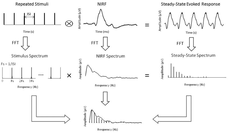
Illustration of the SSVEP spectral analysis. When the steady-state evoked response can be expressed as the result of convolving the stimuli with an equivalent neural impulse response function, the frequency spectrum of the steady-state evoked response equals the spectrum of the stimuli multiplied by the spectrum of the impulse response. By dividing the spectrum of the steady-state evoked response by the stimulus spectrum at the multiples of the stimulus frequency, discrete samples of the impulse response function represented in the frequency domain were obtained. The summation of these discrete samples represents the discrete integral of this spectral profile.
Moreover, our results indicate that the neural response within V1 has a refractory period of about 0.2 s (Fig. 2.d), which is close to the duration of the event-related V1 source activity itself (Fig. 6.d). This suggests that neurons in V1 can be completely ready to respond to a new stimulus only after they finish processing the preceding stimulus. When the ISI is longer than the neural refractory period, the steady-state neural response can be regarded as the output of a linear time-invariant system.
Vascular Refractory Effect
Since neural response nonlinearity can be ruled out by setting the ISI to be longer than the neural refractory period (e.g. ISI≥0.25 s), our results demonstrate that it is possible for BOLD nonlinearity to have a purely vascular origin. Vascular response nonlinearity reflects a nonlinear neurovascular coupling relationship. Results shown in Fig. 3 indicate that the measured and linearly predicted BOLD signals change disproportionately when 0.25<ISI<4 s. More importantly, this nonlinear vascular response is due to a vascular refractory effect (Cannestra et al., 1998; Huettel and McCarthy, 2000; Zhang et al., 2008b), as opposed to a vascular ceiling effect (Bruhn et al., 1994; Buxton et al., 2004). This conclusion is strongly evidenced by our finding that the vascular response nonlinearity depends exclusively on the ISI and is independent of the absolute BOLD response level (Fig. 5). It does not necessarily imply that the BOLD response can go unbounded. Instead, the upper limit (or “ceiling”) may be far beyond the dynamic range of the BOLD signal changes in our experiments and perhaps in most other fMRI experiments as well.
In line with previous studies (Cannestra et al., 1998; Zhang et al., 2008b), our results also suggest that the refractory effect in vascular responses can be uncoupled from any neural origin. As reported here, the vascular refractory period of 4.2 s is much longer than the corresponding neural refractory period of 0.2 s. While the mechanism underlying the vascular refractory effect remains elusive, previous modeling and simulation studies have proposed a variety of hypotheses regarding the interplay among all hemodynamic parameters (Buxton et al., 2004; Friston et al., 2000). In addition, a recent study suggests that vascular nonlinearity depends largely on the local vasculature and on large vessels in particular (Zhang et al., 2008b).
In fact, the non-monotonic relationship between the visual flicker rate and the induced fMRI response has also been reported by several previous studies (e.g. Fox and Raichle, 1985; Kwong et al., 1992; Muthukumaraswamy and Singh, 2008). However, the source of such non-monotonic relationship has not been elucidated by these studies, while it may reflect a disproportional increase in neural activity with the increase in flicker rate (i.e. more trials) or a disproportional increase in hemodynamic response with the neural activity increase. In line with these studies, the present study has provided additional insights to this issue. Our quantitative analyses indicate that the neural activity increases linearly with the flicker rate increase up to about 5 Hz; the hemodynamic response increases linearly with the flicker rate increase up to about 0.24 Hz; for flicker rates higher than 0.24 Hz, the hemodynamic response fails to increase linearly due to vascular refractory effect.
Neurovascular Coupling
The majority of previous studies have generally been in agreement that the BOLD-fMRI signal is driven primarily by post-synaptic activity (Logothetis et al., 2001; Lauritzen, 2001; Attwell and Iadecola, 2002; Raichle and Mintun, 2006; Viswanathan and Freeman, 2007) rather than pre-synaptic spiking activity (Heeger et al., 2000; Rees et al., 2000; Smith et al., 2002; Mukamel et al., 2005). However, this conclusion is at most qualitative. Caution should be taken when using the amplitude and time course of an fMRI signal to infer those of the underlying neural activity, beyond the conventional use of fMRI in spatial mapping and localization of brain functions.
In this regard, tremendous research efforts have been directed towards the topic of neurovascular coupling linearity, though differing conclusions have been made in different studies. It is important to point out that existing disagreements may be accounted for, at least in part, by the lack of a standard way of defining and quantifying neural and hemodynamic signals before comparing them against a linear or nonlinear model. Substantial variance in the methods of quantifying multimodal signals can be witnessed in the literature. Regarding hemodynamic response, the perfusion or BOLD signal has been quantified as the peak amplitude (Devor et al., 2003; Hewson-Stoate et al., 2005; Huttunen et al., 2008; Ou et al., 2009), the steady-state amplitude (Zhang et al., 2008a), or the time integral (Hoffmeyer et al., 2007; Franceschini et al., 2008; Ogawa et al., 2000), etc. Concerning neural response, EEG, MEG, or local field potential (LFP) has been quantified as the peak amplitude (Arthurs et al., 2000; Franceschni et al., 2008; Ou et al., 2009), the peak-to-peak difference (Zhang et al., 2008a), the integrated amplitude or power during a sustained period of stimulation (Hewson-Stoate et al., 2005; Hoffmeyer et al., 2007; Huttenen et al., 2008; Lauritzen, 2001; Sheth et al., 2004), or the integrated amplitude or power during an event-related period following a single stimulus (Devor et al., 2003; Wan et al., 2006). It is questionable whether an arbitrary pair of the above quantitative methods is appropriate to address the cross-modal relationship, or whether a conclusion based on such quantifications is indeed able to reflect the nature of neurovascular coupling.
A unique contribution of the present study also lies in the rigorous derivation of a pair of metrics used for quantifying the BOLD-fMRI and synaptic current activities. The fMRI signal was quantified by the BOLD effect size, defined as the ratio between the measured BOLD signal change and a linear regressor derived from the stimuli. The synaptic current activity was quantified by the integrated power during the event-related period following a single stimulus. According to our theoretical modeling, this pair of metrics should be proportional to each other given a linear neurovascular coupling. Therefore, it provides a principled, and perhaps unique, way to test the hypothesis of linear neurovascular coupling. Note that our results also demonstrate that even if neurovascular coupling is nonlinear due to a purely vascular refractory effect, the linear relationship between the BOLD effect size and the integrated power of the synaptic current should still hold true (Fig. 6.e). This is because the vascular refractory effect only scales the BOLD effect size by a factor dependent on the ISI. After the scaling, the linear cross-modal relationship does not change, although the proportionate factor does.
Our results (Fig. 6) further suggest that the power of the synaptic current correlates slightly better than the magnitude of the synaptic current with the BOLD signal. This finding is in line with several previous studies in support of a quadratic model for relating the synaptic current with the BOLD response (Devor et al., 2003; Franceschini et al., 2008; Wan et al., 2006). This finding might suggest that the power of the synaptic current is the physical correlate of the metabolic energy demand that drives hemodynamic responses. However, our results still remain preliminary and inconclusive, further studies are needed to address this important issue.
The present study not only sheds light on neurovascular coupling, but also provides a theoretical basis for integrating fMRI and EEG in a principled way (Liu and He, 2008; Liu et al., 2009).
Potentially Confounding Factors
In the present study, the cascaded systems that linked the stimuli to the BOLD response were first studied component by component and then as a whole by using three experimental paradigms. These paradigms were very similar in general, whereas slight differences were intentionally made to better suit the need of the EEG or fMRI signal characterization and to better serve to individually address neural response nonlinearity, vascular response nonlinearity and the quantitative relationship between the BOLD effect size and the integrated power of event-related synaptic current.
For instance, sustained full-screen visual stimuli were used to assess the neural response linearity, whereas a (lower-right) quarter hemi-field stimulus was used to study the vascular response linearity and the relationship between the evoked BOLD effect size and the event-related synaptic current response. The different stimulus locations and sizes were designed in consideration of the retinotopic relationship. The upper (or lower) visual field projected to the lower (or upper) portion of the calcarine fissure within the primary visual cortex. A hemi-field stimulus produced a tangential dipole, generating a dipolar scalp potential field dependent on the morphology of the calcarine fissure. Such a dipolar potential pattern would make it rather difficult to select a single channel or a common (among all subjects) sub-set of multiple channels for the EEG signal quantification in the steady state with fast stimulus repetition. In contrast, a full-field stimulus induced electrical currents at both sides of the calcarine fissure within both hemispheres. The net effect was a radial dipole, producing a single focal area of potential distribution with the peak around the central occipital electrode Oz. This feature largely simplified the quantification of steady-state neural response when using the Fourier analysis for the assessment of the neural response linearity.
However, the quarter hemi-field stimulus was preferable when assessing the quantitative relationship between the BOLD effect size and the integrated power of event-related synaptic current. As mentioned above, a full-field stimulus would induce opposing synaptic currents flowing in directions perpendicular to the two banks of the calcarine fissure. The opposing currents would partially cancel each other. A current dipole could only represent the net current as the vector sum of synaptic currents within a ROI, whereas the BOLD response averaged within the same ROI should be independent of the morphology of the fissure that the ROI contained. Therefore, we chose to confine the stimulus to a quarter of the visual field to avoid current cancellation in the assessment of the fMRI-EEG coupling relationship. Note that the issue of opposing currents was not of concern in studying the neural refractory effect, which depended on the relative EEG signal changes with respect to the stimulus timing (i.e. ISI).
Nevertheless, the different stimulus designs might still be thought to potentially confound the generalization of the conclusion drawn from one experimental paradigm to another paradigm. We would like to argue that the conclusions drawn from the three paradigms were mutually confirmative rather than dependent. Perhaps, the only exception was the selection of the ISI range in the Paradigm 2 for the assessment of vascular response nonlinearity. Since we wanted to selectively assess the linearity of hemodynamic response to neural activity, we chose a range of ISI values from 0.25 to 6 sec to presumably ensure the linearity of stimulus-evoked neural response, as we revealed from the Paradigm 1 a neural refractory effect when ISI<0.2 sec. Although it was not unlikely that the neural refractory period might potentially vary due to the different stimulus sizes used in the two paradigms. It was reasonable to expect such stimulus-size dependent variation was too small, if any at all, to invalidate the conclusion that the BOLD response nonlinearity could be caused by a pure nonlinear vascular effect, which was found to be present when the ISI was shorter than 4 sec.
In addition, the Paradigm 3 tested a hypothesis derived from the model (Fig. 1.B) – that is, the BOLD effect size is proportional to the integrated power of event-related synaptic current. Although the model was formed based on the conditions and findings obtained through the Paradigm 1 and Paradigm 2, this model and the relationship derived from it were aimed to be generalizable. Therefore, to test it, we did not necessarily have to use the exactly same paradigm as in Paradigm 1 and Paradigm 2, but indeed used a similar paradigm (Paradigm 3). As we confirmed the validity of our model-derived hypothesis in the primary visual cortex, it also lent supports to the conclusions about the neural and vascular refractory effects. It awaits future studies to evaluate the validity of the proposed model in explaining data from other systems (e.g. sensory-motor systems) by using different stimulus or task.
In the separate sessions of fMRI and EEG recordings in the Paradigm 3, the stimulus was made identical in terms of the stimulus frequency, location and size, except that the stimulus was presented onto a monitor for the EEG-alone session but through a back-mirrored projection for the fMRI session. To ensure that the cross-session difference did not confound our finding, we also acquired the fMRI and EEG in half of the subjects and found the same linear relationship between the BOLD effect size and the integrated power of event-related synaptic current.
It is also worth noting that different task and analysis designs were used to assess the range of ISI within which the linearity of neural and hemodynamic responses fails. A long period of sustained stimuli was used to produce stead-state neural response, which was assessed using spectral analysis. The fMRI response was generated by 30-s blocks of sustained stimuli interleaved with 30-s blocks of baseline, and the blocked fMRI response was quantified as the BOLD effect size. Such a distinction stems from methodological considerations. As previously mentioned, the spectral analysis provides an effective (and perhaps unique way) to assess the stimulus-evoked neural response linearity when stimuli are too close to separate their individual responses in time. The block design gives rise to sufficient signal-to-noise ratio to reliably assess the fMRI response. Most importantly, block-design fMRI response and event-related electrophysiological response, although occurring at highly different time scales, can be quantitatively linked through the system modeling as described in the Method section and our previous paper (Liu and He, 2008).
Although the different task designs and separate EEG-fMRI acquisition seem to make it less straightforward to combine our models expressed in Eqs (6) and (7), which accounted for neural and vascular response nonlinearities respectively, into an integrated model as shown in Fig. 1.B. These models serve as the preliminary mathematical approximations, while future studies are needed to elucidate the detailed physiological mechanism underlying the data and phenomena observed in the present study.
In a previous study (Norcia et al., 2004), it has been suggested that the luminance (or gain) of visual grating stimulation presented on a LCD projector may decrease with increasing temporal frequency. Although it remains unclear if this conclusion would be generalized to all kinds of LCD/DLP displays or projectors, it might be a potentially confounding factor to the interpretation of the neural refractory effect reported in the present study. Since the visual evoked response is generally reduced with decreasing luminance of the visual stimulation, the deviation from the linearity of steady-state neural response at shorter ISIs may be partly explained by the reduced luminance of stimuli at higher frequencies. Therefore, it might be possible that the actual neural refractory period is even shorter than the 0.2 s. However, this potential uncertainty does not affect the interpretation of our results regarding the vascular response nonlinearity, since we used the ISI values larger 0.25 s in all fMRI experiments to assure that the ISI was longer than the neural refractory period so that the neural response is indeed linear.
A high flicker rate may likely induce motion perception and the underlying neural activity may likely contain both the patter-reversal evoked response and the motion-perception-related response (Grossberg and Rudd, 1992). However, the motion-perception-related response mainly occurs in the motion-sensitive area (MT+) instead of the primary visual cortex, to which our EEG and fMRI analyses are confined. Our EEG data demonstrate that the steady-state response induced by fast stimuli with the flicker rate up to about 5 Hz can be well predicted by convolving the stimuli with the single-trial response obtained with the flicker rate as low as 0.5 Hz, which should not induce motion perception. This further supports our argument that neural response at the primary visual cortex is not affected by the motion perception, at least for the flicker rate lower than 5 Hz.
Acknowledgments
The authors are thankful to Ms. Han Yuan for helpful discussions, and Mr. Daniel Schober and Ms. Diana Groschen for assistance in EEG data collection. This work was supported by NIH RO1EB007920, RO1EB006433, a grant from the Institute for Engineering in Medicine of the University of Minnesota, and a grant from the Minnesota Partnership for Biotechnology and Medical Genomics. The 3T scanner is supported in part by NIH P41RR008079 and P30NS057091.
Appendix: SSVEP Spectral Analysis
To test the neural response linearity, a SSVEP spectral analysis was performed in the present study. Here, we describe the theoretical details with respect to this method.
The hypothesis tested is described as follows.
| (A.1) |
where y(Δ,t) represents the measured SSVEP signal in response to repeated stimuli with a variable ISI (denoted as Δ). z(Δ,t) represents the prediction of the SSVEP signal by assuming the SSVEP signal is a linear function with respect to the stimulus.
By definition, the linearly predicted SSVEP signal can be represented by convolving the external stimuli, denoted as x(Δ,t), with a time-invariant system φ(t). In the present study, the convolution kernel was assumed to be the VEP (or ERP) signal obtained when the ISI was set to be 2 seconds.
| (A.2) |
To model the repetitive stimuli, we define x(Δ,t) as a train of delta functions.
| (A.3) |
The measured SSVEP signal obtained with variable ISI is always pseudo-periodic, as manifested by the peaks at multiples of the stimulus frequency in the EEG spectrum. Therefore, the measured SSVEP signal can be represented by convolving the stimulus function with an unknown equivalent impulse response function (EIRF), which may vary at different ISI values. Such frequency specificity, known as “frequency tagging” as well, also allows us to distinguish the SSVEP signal from the background noise.
| (A.4) |
where κ(Δ,t) represents the unknown EIRF specific to each ISI value.
Testing Eq. (A.1) is equivalent to testing Eq. (A.5), which describes a hypothesis that the EIRF is independent of the ISI and always equals the VEP signal.
| (A.5) |
It must be noted that κ(Δ,t) is rather difficult to extract from the measured SSVEP signals when the ISI is too short, since the single-trial responses to adjacent stimuli in overlap with each other. To bypass this challenge, we compare the EIRF and the VEP in the frequency domain, instead of in the time domain.
In other words, instead of testing Eq. (A.5), we test Eq. (A.6).
| (A.6) |
where K(Δ,ω) and Φ(ω) result from the Fourier transform of κ(Δ,t) and φ(t) respectively, and ω stands for frequency.
Transforming both sides of Eq. (A.2) and Eq. (A.4) into the frequency domain gives rise to Eq. (A.7) and Eq. (A.8), respectively.
| (A.7) |
| (A.8) |
where X(Δ,ω), Y(Δ,ω) and Z(Δ,ω) results from the Fourier transform of the stimulus function, the measured and linearly predicted SSVEP signals, respectively. Importantly, since the stimulus function is a train of delta functions separated by the ISI, the frequency spectrum of the stimulus function also appears as a train of spikes, not necessarily of equal heights, separated by the stimulus frequency, defined as ωΔ =1/Δ (here, the notation, ωΔ, represents a frequency value as a function ISI).
Based on Eq. (A.7) and Eq. (A.8), discrete samples of the amplitudes of Φ(ω) and K(Δ,ω) at multiples of ωΔ (i.e. ωΔ, 2ωΔ, 3ωΔ, …) can be computed by using Eq. (A.9) and Eq. (A.10), respectively.
| (A.9) |
| (A.10) |
where i = 1, 2, …
We can sum these discrete samples (up to 40 Hz) and compute the ratio between the summed results (namely the RCC value as defined in the main text), and expressed this ratio as a function of the ISI, denoted as Γ(Δ) in Eq. (A.11).
| (A.11) |
For a specific value of the ISI, if the RCC value equals one, we accept the hypothesis that the neural response is linear. If the RCC value is smaller than one, meaning that the equivalent impulse response function has smaller amplitudes than the assumed ISI-independent impulse response function, it suggests a neural refractory effect of decreased neural response due to a suppressive interaction between closely elicited neuronal events. If the RCC value is larger than one, meaning that the equivalent impulse response function has larger amplitudes than the hypothetical impulse response function, it suggests a neural facilitative effect of increased neural response due to a facilitative interaction between closely elicited neuronal events.
The spectral analysis described above is further illustrated by Fig. 7.
References
- Allen PJ, Josephs O, Turner R. A method for removing imaging artifact from continuous EEG recorded during functional MRI. Neuroimage. 2000;12:230–239. doi: 10.1006/nimg.2000.0599. [DOI] [PubMed] [Google Scholar]
- Allen PJ, Polizzi G, Krakow K, Fish DR, Lemieux L. Identification of EEG events in the MR scanner: The problem of pulse artifact and a method for its subtraction. Neuroimage. 1998;8:229–239. doi: 10.1006/nimg.1998.0361. [DOI] [PubMed] [Google Scholar]
- Arthurs OJ, Williams EJ, Carpenter TA, Pickard JD, Boniface SJ. Linear coupling between functional magnetic resonance imaging and evoked potential amplitude in human somatosensory cortex. Neuroscience. 2000;101:803–806. doi: 10.1016/s0306-4522(00)00511-x. [DOI] [PubMed] [Google Scholar]
- Attwell D, Iadecola C. The neural basis of functional brain imaging signals. Trends Neurosci. 2002;25:621–625. doi: 10.1016/s0166-2236(02)02264-6. [DOI] [PubMed] [Google Scholar]
- Bandettini PA, Wong EC, Hinks RS, Tikofsky RS, Hyde JS. Time course EPI of human brain function during task activation. Magn Reson Med. 1992;25:390–397. doi: 10.1002/mrm.1910250220. [DOI] [PubMed] [Google Scholar]
- Birn RM, Bandettini PA. The effect of stimulus duty cycle and “off” duration on BOLD response linearity. Neuroimage. 2005;27:70–82. doi: 10.1016/j.neuroimage.2005.03.040. [DOI] [PubMed] [Google Scholar]
- Boynton GM, Engel SA, Glover GH, Heeger DJ. Linear systems analysis of functional magnetic resonance imaging in human V1. J Neurosci. 1996;16:4207–4221. doi: 10.1523/JNEUROSCI.16-13-04207.1996. [DOI] [PMC free article] [PubMed] [Google Scholar]
- Bruhn H, Kleinschmidt A, Boecker H, Merboldt KD, Hanicke W, Frahm J. The effect of acetazolamide on regional cerebral blood oxygenation at rest and under stimulation as assessed by. MRI J Cereb Blood Flow Metab. 1994;14:742–748. doi: 10.1038/jcbfm.1994.95. [DOI] [PubMed] [Google Scholar]
- Budd TW, Barry RJ, Gordon E, Rennie C, Michie PT. Decrement of the N1 auditory event-related potential with stimulus repetition: Habituation vs. refractoriness. Int J Psychophysiol. 1998;31:51–68. doi: 10.1016/s0167-8760(98)00040-3. [DOI] [PubMed] [Google Scholar]
- Buxton RB, Uludag K, Dubowitz DJ, Liu TT. Modeling the hemodynamic response to brain activation. Neuroimage. 2004;23:S220–S233. doi: 10.1016/j.neuroimage.2004.07.013. [DOI] [PubMed] [Google Scholar]
- Cannestra AF, Pouratian N, Shomer MH, Toga AW. Refractory periods observed by intrinsic signal and fluorescent dye imaging. J Neurophysiol. 1998;80:1522–1532. doi: 10.1152/jn.1998.80.3.1522. [DOI] [PubMed] [Google Scholar]
- Cohen MS. Parametric analysis of fMRI data using linear systems methods. Neuroimage. 1997;6:93–103. doi: 10.1006/nimg.1997.0278. [DOI] [PubMed] [Google Scholar]
- Dale AM, Buckner RL. Selective averaging of rapidly presented individual trials using fMRI. Hum Brain Mapp. 1997;5:329–340. doi: 10.1002/(SICI)1097-0193(1997)5:5<329::AID-HBM1>3.0.CO;2-5. [DOI] [PubMed] [Google Scholar]
- de Zwart JA, van Gelderen P, Jansma JM, Fukunaga M, Bianciardi M, Duyn JH. Hemodynamic nonlinearities affect BOLD fMRI response timing and amplitude. NeuroImage. 2009;47:1649–1658. doi: 10.1016/j.neuroimage.2009.06.001. [DOI] [PMC free article] [PubMed] [Google Scholar]
- Devor A, Dunn AK, Andermann ML, Ulbert I, Boas DA, Dale AM. Coupling of total hemoglobin concentration, oxygenation, and neural activity in rat somatosensory cortex. Neuron. 2003;39:353–359. doi: 10.1016/s0896-6273(03)00403-3. [DOI] [PubMed] [Google Scholar]
- Di Russo F, Pitzalis S, Spitoni G, Aprile T, Patria F, Spinelli D, Hillyard SA. Identification of the neural sources of the pattern-reversal VEP. NeuroImage. 2005;24:874–886. doi: 10.1016/j.neuroimage.2004.09.029. [DOI] [PubMed] [Google Scholar]
- Fox PT, Raichle ME. Stimulus rate determines regional brain blood flow in striate cortex. Ann Neurol. 1985;17:303–305. doi: 10.1002/ana.410170315. [DOI] [PubMed] [Google Scholar]
- Franceschini MA, Nissila I, Wu W, Diamond SG, Bonmassar G, Boas DA. Coupling between somatosensory evoked potentials and hemodynamic response in the rat. Neuroimage. 2008;41:189–203. doi: 10.1016/j.neuroimage.2008.02.061. [DOI] [PMC free article] [PubMed] [Google Scholar]
- Friston KJ, Jezzard P, Turner R. Analysis of functional MRI time series. Hum Brain Mapp. 1994;1:153–171. [Google Scholar]
- Friston KJ, Mechelli A, Turner R, Price CJ. Nonlinear responses in fMRI: The balloon model, volterra kernels, and other hemodynamics. Neuroimage. 2000;12:466–477. doi: 10.1006/nimg.2000.0630. [DOI] [PubMed] [Google Scholar]
- Goebel R, Esposito F, Formisano E. Analysis of functional image analysis contest (FIAC) data with brainvoyager QX: From single-subject to cortically aligned group general linear model analysis and self-organizing group independent component analysis. Hum Brain Mapp. 2006;27:392–401. doi: 10.1002/hbm.20249. [DOI] [PMC free article] [PubMed] [Google Scholar]
- Grossberg S, Rudd ME. Cortical dynamics of visual motion perception: short-range and long-range apparent motion. Psych Rev. 1992;99:78–121. doi: 10.1037/0033-295x.99.1.78. [DOI] [PubMed] [Google Scholar]
- Heeger DJ, Huk AC, Geisler WS, Albrecht DG. Spikes versus BOLD: What does neuroimaging tell us about neuronal activity? Nat Neurosci. 2000;3:631–633. doi: 10.1038/76572. [DOI] [PubMed] [Google Scholar]
- Herman P, Sanganahalli BG, Blumenfeld H, Hyder F. Cerebral oxygen demand for short-lived and steady-state events. J Neurochem. 2009;109:73–79. doi: 10.1111/j.1471-4159.2009.05844.x. [DOI] [PMC free article] [PubMed] [Google Scholar]
- Hewson-Stoate N, Jones M, Martindale J, Berwick J, Mayhew J. Further nonlinearities in neurovascular coupling in rodent barrel cortex. Neuroimage. 2005;24:565–574. doi: 10.1016/j.neuroimage.2004.08.040. [DOI] [PubMed] [Google Scholar]
- Hoffmeyer HW, Enager P, Thomsen KJ, Lauritzen MJ. Nonlinear neurovascular coupling in rat sensory cortex by activation of transcallosal fibers. J Cereb Blood Flow Metab. 2007;27:575–87. doi: 10.1038/sj.jcbfm.9600372. [DOI] [PubMed] [Google Scholar]
- Huettel SA, McCarthy G. Evidence for a refractory period in the hemodynamic response to visual stimuli as measured by MRI. Neuroimage. 2000;11:547–553. doi: 10.1006/nimg.2000.0553. [DOI] [PubMed] [Google Scholar]
- Huttunen JK, Grohn O, Penttonen M. Coupling between simultaneously recorded BOLD response and neuronal activity in the rat somatosensory cortex. Neuroimage. 2008;39:775–785. doi: 10.1016/j.neuroimage.2007.06.042. [DOI] [PubMed] [Google Scholar]
- Kwong KK, Belliveau JW, Chesler DA, Goldberg IE, Weisskoff RM, Poncelet BP, Kennedy DN, Hoppel BE, Cohen MS, Turner R. Dynamic magnetic resonance imaging of human brain activity during primary sensory stimulation. Proc Natl Acad Sci U S A. 1992;89:5675–5679. doi: 10.1073/pnas.89.12.5675. [DOI] [PMC free article] [PubMed] [Google Scholar]
- Lauritzen M. Relationship of spikes, synaptic activity, and local changes of cerebral blood flow. J Cereb Blood Flow Metab. 2001;21:1367–1383. doi: 10.1097/00004647-200112000-00001. [DOI] [PubMed] [Google Scholar]
- Liu Z, He B. fMRI–EEG integrated cortical source imaging by use of time-variant spatial constraints. NeuroImage. 2008;39:1198–1214. doi: 10.1016/j.neuroimage.2007.10.003. [DOI] [PMC free article] [PubMed] [Google Scholar]
- Liu Z, Zhang N, Chen W, He B. Mapping the Bilateral Visual Integration by EEG and fMRI. NeuroImage. 2009 doi: 10.1016/j.neuroimage.2009.03.028. [DOI] [PMC free article] [PubMed] [Google Scholar]
- Logothetis NK. What we can do and what we cannot do with fMRI. Nature. 2008;453:869–878. doi: 10.1038/nature06976. [DOI] [PubMed] [Google Scholar]
- Logothetis NK, Pauls J, Augath M, Trinath T, Oeltermann A. Neurophysiological investigation of the basis of the fMRI signal. Nature. 2001;412:150–157. doi: 10.1038/35084005. [DOI] [PubMed] [Google Scholar]
- Martindale J, Mayhew J, Berwick J, Jones M, Martin C, Johnston D, Redgrave P, Zheng Y. The hemodynamic impulse response to a single neural event. J Cereb Blood Flow Metab. 2003;23:546–55. doi: 10.1097/01.WCB.0000058871.46954.2B. [DOI] [PubMed] [Google Scholar]
- Mukamel R, Gelbard H, Arieli A, Hasson U, Fried I, Malach R. Coupling between neuronal firing, field potentials, and FMRI in human auditory cortex. Science. 2005;309:951–954. doi: 10.1126/science.1110913. [DOI] [PubMed] [Google Scholar]
- Muller JR, Metha AB, Krauskopf J, Lennie P. Rapid adaptation in visual cortex to the structure of images. Science. 1999;285:1405–1408. doi: 10.1126/science.285.5432.1405. [DOI] [PubMed] [Google Scholar]
- Muthukumaraswamy SD, Singh KD. Spatiotemporal frequency tuning of BOLD and gamma band MEG responses compared in primary visual cortex. Neuroimage. 2008;40:1552–1560. doi: 10.1016/j.neuroimage.2008.01.052. [DOI] [PubMed] [Google Scholar]
- Nangini C, Tam F, Graham SJ. A novel method for integrating MEG and BOLD fMRI signals with the linear convolution model in human primary somatosensory cortex. Hum Brain Mapp. 2008;29(1):97–106. doi: 10.1002/hbm.20361. [DOI] [PMC free article] [PubMed] [Google Scholar]
- Norcia AM, McKee SP, Bonneh Y, Pettet MW. Suppression of monocular visual direction under fused binocular stimulation: evoked potential measurements. J Vis. 2005;5(1):34–44. doi: 10.1167/5.1.4. [DOI] [PubMed] [Google Scholar]
- Ogawa S, Lee TM, Stepnoski R, Chen W, Zhu XH, Ugurbil K. An approach to probe some neural systems interaction by functional MRI at neural time scale down to milliseconds. Proc Natl Acad Sci U S A. 2000;97:11026–11031. doi: 10.1073/pnas.97.20.11026. [DOI] [PMC free article] [PubMed] [Google Scholar]
- Ogawa S, Tank DW, Menon R, Ellermann JM, Kim SG, Merkle H, Ugurbil K. Intrinsic signal changes accompanying sensory stimulation: Functional brain mapping with magnetic resonance imaging. Proc Natl Acad Sci U S A. 1992;89:5951–5955. doi: 10.1073/pnas.89.13.5951. [DOI] [PMC free article] [PubMed] [Google Scholar]
- Ou W, Nissila I, Radhakrishnan H, Boas DA, Hamalainen MS, Franceschini MA. Study of neurovascular coupling in humans via simultaneous magnetoencephalography and diffuse optical imaging acquisition. NeuroImage. 2009;46:624–632. doi: 10.1016/j.neuroimage.2009.03.008. [DOI] [PMC free article] [PubMed] [Google Scholar]
- Raichle ME, Mintun MA. Brain work and brain imaging. Annu Rev Neurosci. 2006;29:449–76. doi: 10.1146/annurev.neuro.29.051605.112819. [DOI] [PubMed] [Google Scholar]
- Rees G, Friston K, Koch C. A direct quantitative relationship between the functional properties of human and macaque V5. Nat Neurosci. 2000;3:716–723. doi: 10.1038/76673. [DOI] [PubMed] [Google Scholar]
- Sheth SA, Nemoto M, Guiou M, Walker M, Pouratian N, Toga AW. Linear and nonlinear relationships between neuronal activity, oxygen metabolism, and hemodynamic responses. Neuron. 2004;42:347–355. doi: 10.1016/s0896-6273(04)00221-1. [DOI] [PubMed] [Google Scholar]
- Smith AJ, Blumenfeld H, Behar KL, Rothman DL, Shulman RG, Hyder F. Cerebral energetics and spiking frequency: The neurophysiological basis of fMRI. Proc Natl Acad Sci U S A. 2002;99:10765–10770. doi: 10.1073/pnas.132272199. [DOI] [PMC free article] [PubMed] [Google Scholar]
- Vanni S, Warnking J, Dojat M, Delon-Martin C, Bullier J, Segebarth C. Sequence of pattern onset responses in the human visual areas: an fMRI-constrained VEP source analysis. NeuroImage. 2004;21:801–817. doi: 10.1016/j.neuroimage.2003.10.047. [DOI] [PubMed] [Google Scholar]
- Vazquez AL, Noll DC. Nonlinear aspects of the BOLD response in functional MRI. Neuroimage. 1998;7:108–118. doi: 10.1006/nimg.1997.0316. [DOI] [PubMed] [Google Scholar]
- Viswanathan A, Freeman RD. Neurometabolic coupling in cerebral cortex reflects synaptic more than spiking activity. Nat Neurosci. 2007;10:1308–1312. doi: 10.1038/nn1977. [DOI] [PubMed] [Google Scholar]
- Wan X, Riera J, Iwata K, Takahashi M, Wakabayashi T, Kawashima R. The neural basis of the hemodynamic response nonlinearity in human primary visual cortex: Implications for neurovascular coupling mechanism. Neuroimage. 2006;32:616–625. doi: 10.1016/j.neuroimage.2006.03.040. [DOI] [PubMed] [Google Scholar]
- Zhang N, Liu Z, He B, Chen W. Noninvasive study of neurovascular coupling during graded neuronal suppression. J Cereb Blood Flow Metab. 2008a;28:280–290. doi: 10.1038/sj.jcbfm.9600531. [DOI] [PubMed] [Google Scholar]
- Zhang N, Zhu XH, Chen W. Investigating the source of BOLD nonlinearity in human visual cortex in response to paired visual stimuli. NeuroImage. 2008b;43:204–12. doi: 10.1016/j.neuroimage.2008.06.033. [DOI] [PMC free article] [PubMed] [Google Scholar]