Optimal reward harvesting in complex perceptual environments

Abstract

The ability to choose rapidly among multiple targets embedded in a complex perceptual environment is key to survival. Targets may differ in their reward value as well as in their low-level perceptual properties (e.g., visual saliency). Previous studies investigated separately the impact of either value or saliency on choice; thus, it is not known how the brain combines these two variables during decision making. We addressed this question with three experiments in which human subjects attempted to maximize their monetary earnings by rapidly choosing items from a brief display. Each display contained several worthless items (distractors) as well as two targets, whose value and saliency were varied systematically. We compared the behavioral data with the predictions of three computational models assuming that (i) subjects seek the most valuable item in the display, (ii) subjects seek the most easily detectable item, and (iii) subjects behave as an ideal Bayesian observer who combines both factors to maximize the expected reward within each trial. Regardless of the type of motor response used to express the choices, we find that decisions are influenced by both value and feature-contrast in a way that is consistent with the ideal Bayesian observer, even when the targets’ feature-contrast is varied unpredictably between trials. This suggests that individuals are able to harvest rewards optimally and dynamically under time pressure while seeking multiple targets embedded in perceptual clutter.

Animals and humans often need to make rapid choices among multiple targets embedded in a noisy perceptual environment. Consider, for example, a predator deciding which of several prey to pursue. The more valuable targets might be perceptually less salient, and thus harder to find (e.g., camouflaged prey), while less valuable targets may be perceptually more salient and easier to find. To solve this task, the animal needs to combine the perceptual and value-related information while making choices. This raises a fundamental question: Are rapid choices in cluttered environments dominated by value information (e.g., biased toward seeking the more valuable items) or by perceptual information (e.g., biased toward seeking the more easily and quickly detectable items)?

Understanding how perceptual saliency and value information are combined to make decisions is important for several reasons. From a computational perspective, it is not known how the brain trades off saliency and value under time pressure, especially when they have opposing influences on the decision: Is it optimized for reward harvesting, or is it based on simpler principles of choosing the most valuable or the most easily detectable item? The brain's solution to this tradeoff is not obvious, because items that are more salient are easier to find (1, 2) and, other things being equal, have a higher probability of yielding a reward. From a behavioral perspective, it is not known whether humans take into account saliency-induced variations in probability when making decisions under uncertainty. From a vision science perspective, previous research on visual search has focused on searching for a single target amid clutter (2, 3), and it is not known what happens when subjects search for multiple targets that differ both in saliency and in value. In particular, although saliency is known to affect saccades in a fast, automatic, and bottom-up manner (4), it is not known whether value can have a similar fast effect.

Previous studies have examined the roles of visual saliency and economic or subjective value in isolation. For example, several studies showed that decisions are biased toward the item or location associated with a higher magnitude and probability of reward (5–8), but these studies did not manipulate visual saliency. On the other hand, studies on visual saliency did not manipulate the reward outcome associated with choosing an item. These studies showed that during free viewing of natural scenes and videotapes, saccades are automatically drawn to more salient image regions (e.g., locations with high feature-contrast in luminance, orientation, and motion) (9–13) and that salient targets are detected faster and better amid clutter (1, 2). Thus, whether and how the brain might combine information about visual saliency and value to form rapid decisions have not yet been investigated.

To study this question, we collected data from a number of human subjects who searched visually for two valuable targets amid clutter. The goal of our subjects was to maximize the reward earned by rapidly choosing items from a brief display (Fig. 1A). We systematically varied the relative value and feature-contrast of the targets (a measure of saliency based on the difference in features between the target and distractor) across blocks and studied how our subjects’ behavior changed as a consequence. We tested three possible models of our subjects’ behavior. The first model is motivated by the literature on visual search; it assumes that subjects will attempt to select the most salient or easily detectable target based on visual properties of the targets (1, 14). The second model is motivated by the literature on economics; it assumes that subjects attempt to select the most valuable target based on the economic properties of the targets (5). The third model assumes that the brain dynamically combines information about value and visual saliency to select the location that gives the maximum expected reward.

Fig. 1.

Basic experiment and competing theories. (A) Experiment 1. Stimuli in the display were either “targets” or “distractors.” Subjects earned a reward for fixating a target for at least 100 ms during the display period but did not earn a reward for fixating a distractor. There were two types of targets, horizontal bars (H) and vertical bars (V), and one of each was present in each display. Distractors were diagonal bars whose orientation was varied across blocks to manipulate the “feature-contrast” of the targets (orientation difference between the target and distractors). Subjects expressed their choice by fixating on the chosen item and were asked to try to maximize their total earnings. The experiment consisted of several blocks of 50 trials. Across blocks, we varied the value and feature-contrast of the targets. At the beginning of each block, subjects were informed about the value of targets H and V (e.g., value of H is 20 points, value of V is 10 points), and they received training. (B) We compared the performance of three different computational models. In M1, fixations are deployed to the location that is most likely to contain the target with the maximum feature-contrast for the block. In M2, fixations are deployed to the location that is most likely to contain the target associated with the highest value for the block. In M3, fixations are deployed to the location associated with the maximum expected reward for the trial, as predicted by an ideal Bayesian observer model.

Note that it is not possible to choose a priori, or based on existing data, one of the three models. Model 1 is motivated by the fact that the brain might not have sufficient time to incorporate reward considerations during rapid decisions, which would imply that rapid choices would be driven mostly by the perceptual features of the display. Model 2 is motivated by the fact that because the organism cares only about maximizing the amount of rewards harvested, the brain might have implemented a computational shortcut of always attempting to select the highest value stimuli (e.g., always seek the most valuable prey). Model 3 is the optimal solution to the computational problem faced by the organism, and thus is of particular interest.

Results

Decision Models.

Our models are represented schematically in Fig. 1B. All three models first estimate the location of both targets. This estimate is probabilistic, and it is carried out using the optimal Bayesian estimator. All models assume that noisy estimates of the stimulus feature (e.g., orientation, brightness) are computed at each location x. We hypothesize a diverse population of orientation-tuned mechanisms at each location whose output may be converted into a noisy estimate of the stimulus orientation, wherein the noise is approximately Gaussian (15). Formally, let T_x be the stimulus, θ(T_x) be the stimulus feature, and a_x be the estimate of the stimulus feature at location x. Thus, a_x|T_x ∼ G[a_x;μ = θ(T_x), σ], where σ is the noise parameter, and G(·;μ, σ) denotes the univariate Gaussian probability density function with the mean equal to μ and the SD equal to σ. All three models involve a single free parameter, σ. We denote the resulting vector of estimates at eight locations in the display as .

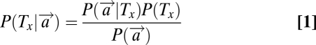
All models require the computation of posterior probabilities. The posterior probability of stimulus T_x occurring at location x is denoted by and is computed from the likelihood and a prior probability P(T_x) using Bayes’ theorem. If the display consists of n stimuli (two targets, H and V, as well as n-2 distractors, D), and if the probability that any stimulus occupies any position is the same, then we have that

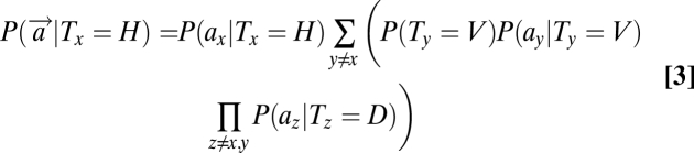
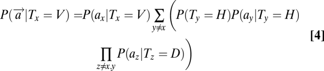
The likelihood term can be further expanded to make use of the fact that exactly one H and one V appear in the display. Thus, the occurrence of H at location x implies that V must occur at some other location y ≠ x and the distractors must appear at other locations z ≠ x, y. It follows that

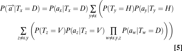A detailed derivation of these equations is presented in SI Text. The terms on the left denote the global likelihood of an item's presence (target/distractor) at location x based on the sensory observations at all locations. In contrast, the terms on the right refer to the local likelihoods of an item's presence at a location based on the sensory observation at that single location, P(a_x|T_x). Substituting Eq. 3–5 in Eq. 1, we can obtain the posterior probability of each object's presence at each location.

The first model (M1) assumes that the decision is dominated by visual properties like feature-contrast (16, 17). In this model, subjects use their prior knowledge of which of the two targets (H or V) is more salient (learned during the 10 training trials preceding each block) and then search for that target when the display appears. Suppose, for instance, that the more salient target is V; according to this model, subjects will choose the location x, where is maximal.

The second model (M2) assumes that the decision is dominated by economic properties of the targets (5), such as value. Here, subjects determine in advance (from the 10 training trials) which of the two targets (H or V) has the higher payoff and then search for that target when the display appears. For example, consider a condition for Fig. 1A in which fixating on the horizontal bar pays 20 points, fixating on the vertical bar pays 10 points, and fixating on the distractors pays nothing. In this case, the model assumes that subjects will search for the horizontal bar and will find it with a higher probability if it is more salient and with a lower probability otherwise. More formally, if the most valuable target is H, then subjects, according to this model, will choose the location x where is maximal.

The third model (M3) has not been previously considered in the search literature. It assumes that the subject computes the expected reward associated with choosing each location using optimal Bayesian inference and then chooses the location with the highest expected reward. We refer to this model as the reward maximizer because it optimizes the expected reward trial-by-trial, given the noise in the system. Note that, unlike M1 and M2, M3 predicts that subjects will not search for a fixed target (e.g., horizontal); instead, they will select dynamically and image-by-image the location of maximum expected reward. More formally, the model assumes that subjects compute the expected reward at every location x, denoted as E[R_x] and then choose the location associated with the highest expected reward. The expected reward at a location is given by

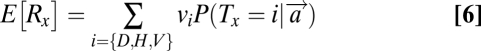where v_i denotes the value associated with the item and is computed as in Eq. 1.

Experiment 1.

This experiment investigates how the brain combines feature-contrast and value information about objects when subjects express their choice by moving their eyes. The feature-contrast and value of the targets were manipulated independently. As illustrated in Fig. 1A and described in Methods, the subjects’ task was to harvest the maximum possible amount of monetary rewards by fixating items in the display.

Fig. 2 A–D displays the performance data for one subject across different relative value conditions (Figs. S1–S5 provide the data from the remaining subjects). The figure illustrates two patterns that were present in all the subjects. First, the probability of fixating on H increases with its relative feature-contrast for all values of the targets. Second, the probability of fixating on H also increases with its relative value.

Fig. 2.

Results for experiment 1. (A–D) Each panel shows the data for subject 1 in a different value condition as a function of the ratio of feature-contrast of the targets. Each dot refers to the frequency of fixations on target H under the particular value and feature-contrast parameters; the error bar denotes the SE. Each panel also shows the predictions made by the three models (model parameters were estimated using data in C and were used to generate predictions in A, B, and D) and the χ² goodness-of-fit statistic for each of the models. In all cases, the ideal observer model (M3) accounts best for the data. (E) Plot of each model's predictions for all 28 experimental conditions vs. a subject's peformance. Each dot represents the frequency of fixations on target H in a different value and feature-contrast condition, as observed in the subject's data and as predicted by the model. (F) Bayesian model comparison. In all six subjects, M1 (light gray) and M2 (dark gray) have a lower likelihood of generating the data than the ideal observer model (M3).

For each subject and model, we determined the maximum-likelihood estimate of the internal noise parameter (σ) from the data in the high-value condition (in which target H is twice as valuable as V; Fig. 2C) and used it to predict behavior in three other value conditions (Fig. 2 A, B, and D and Methods provide details). Fig. 2 A–D compares the predictions of the models with subjects’ data. Note a few things about the predictions made by the models. First, all of them predict that the frequency of fixations to H should increase with its feature-contrast. Second, model M1 predicts that fixations are independent of the values (M1 curves are identical across Fig. 2 A–D), although the data appear to shift gradually from right (Fig. 2A) to left (Fig. 2D). Third, model M2 predicts that the less valuable target will almost never be fixated, even if it has higher feature-contrast; this prediction is clearly violated (Fig. 2A, notice that the M2 curve is constant at zero over the whole feature-contrast range). Fourth, model M3 not only performs better than models M1 and M2, but, more importantly, it predicts the data well, as shown by a quantitative comparison based on a χ² measure of goodness of fit as well as a Bayesian model comparison (18) of the log likelihood of data given each model (Fig. 2F). This last point is further explored in Fig. 2E, which shows that subjects’ fixations correlate well with the predictions of M3 (R² = 0.97). We can conclude that subjects’ behavior is highly consistent with the reward maximizer model M3 and that both value and feature-contrast affect the saccadic decision.

Experiment 2.

To test if the previous findings are robust to the presence of other types of low-level features, we repeated experiment 1 using brightness intensity, rather than orientation, as the feature differentiating the target from the distractors (Fig. 3 and Methods provide details). We obtained data in 21 conditions (7 feature-contrast × 3 value conditions). Fig. 3 C–E displays the data for one of the subjects (Figs. S6 and S7 provide the data for the remaining subjects). Note that the key findings from the first experiment also hold here: First, the saccadic decision is affected by both value and feature-contrast, and, second, M3 (reward maximizer) provides a quantitative account of subjects’ data.

Fig. 3.

Results for experiment 2. (A) Task is identical to experiment 1 except that the feature-contrast variable that was manipulated was the brightness of the targets relative to the distractors. (B) Correlations. (C) Bayesian model comparison. In all three subjects, M3 had a higher likelihood of explaining the data than M1 or M2. (D-F) Data and model fits for subject 1.

Experiment 3.

The findings from experiments 1 and 2 show that subjects can optimize the reward when the targets’ values and feature-contrast are fixed within a block. One hypothesis for why subjects perform so well is that they may learn the optimal strategy during the training period (10 trials preceding each experimental block) and then deploy this learned strategy in the remaining trials in that block. This raises an important question: Can subjects optimize reward dynamically in the absence of training or learning? To test this, we designed a third experiment in which we varied the targets’ feature-contrast unpredictably between trials as opposed to the blocked condition in experiments 1 and 2.

Another question is whether the findings of experiments 1 and 2 reflect properties specific to the saccadic system or a general property of decision making, regardless of the type of motor response (e.g., key press, saccade, verbal report) used to express the choices. To test this, we allowed subjects to report their decision through either a key press in half of the trials or through a saccade in the other half. We made one key modification in the display response paradigm: Subjects maintained cental fixation while viewing the display for 300 ms. The display was followed by a mask containing a masking stimulus at each location as well as a number from 1 to 8 identifying each location uniquely. Subjects were instructed to report their decision as soon as possible by saccading to the chosen location or by typing on a computer keyboard a number from 1 to 8 to indicate the chosen location (maximum response time was 2 s).

The results across nine conditions (3 value × 3 feature-contrast conditions) are shown in Fig. 4). Fig. 4 B and C shows that decisions, regardless of whether expressed through a key press with a finger or through a saccadic eye movement, are influenced by both value and feature-contrast. Comparing Fig. 4 B and C does not reveal any significant difference (pairwise t tests, 0.05 significance level) between the decisions expressed through a key press or saccade. The surprising finding is that despite trial-by-trial variations in feature-contrast, subjects’ performance is still optimal for decisions expressed through a key press (Fig. 4 D and E) and for decisions expressed through a saccade (Fig. 4 F and G). This rules out constant decision strategies that may result from ample practice or overtraining and shows that subjects are optimizing reward on a trial-by-trial basis by using a dynamic strategy of choosing flexibly different targets between trials rather than a static strategy of choosing the same target on all trials in a block. Thus, Fig. 4 B–G shows clearly that decisions, regardless of the type of motor response (key press vs. saccade), are influenced by both value and feature-contrast optimally.

Fig. 4.

Results for experiment 3. (A) Task is similar to that in experiment 1 except that subjects maintained central fixation for 300 ms while viewing the display, following which they expressed their decision either through a key press (in half of the trials) or a saccade (in the other half) to indicate the chosen location. In addition, the targets’ feature-contrast was varied unpredictably between trials, as opposed to experiments 1 and 2, where it was fixed within the block. (B and C) Panels show how the decisions made by the average subject vary with the targets’ feature-contrast and values when choices were reported through a key press (B) or through a saccade (C). Error bars reflect the SEM detection rate across subjects. (D and E) Model predictions vs. data for decisions expressed through a key press. Comparisons between the three models show that the predictions of the ideal observer model (M3) provide the best fit and correlate best with the data. (F and G) Models are similar to those in D and E except that they represent decisions expressed through a saccade.

Discussion

Although objects in the real world usually differ in both visual saliency and economic value, previous studies on saccades and decisions among multiple objects have mostly examined the effect of saliency (9–13) and value (5–8) in isolation. For example, Platt and Glimcher (5) showed that saccadic decisions are biased toward the item associated with the higher expected reward, but they did not vary the feature-contrast or saliency of items. Similarly, Berg et al. (13) studied how visual saliency affects saccades but did not consider the role of stimulus value or reward outcome associated with the saccade. In contrast, we explored the computational mechanisms by which the brain combines visual saliency and value information to make rapid decisions. Our experimental results show that decisions are affected by both variables in a manner that leads to the maximization of the expected reward within each trial and are consistent with the predictions of an ideal Bayesian observer. We found that such reward maximization behavior is robust across multiple visual features, such as orientation and intensity, and does not depend on the type of motor response used to express the choices (key press vs. saccade). Furthermore, behavior is near-optimal even when the targets’ feature-contrast is varied unpredictably between trials, which suggests that subjects deploy a dynamic decision strategy.

An important open question is where in the brain is the information about value and feature-contrast combined. One hypothesis is that value integration may occur as early as in V1, possibly in the form of a greater top-down attentional bias on the more valuable target (19, 20). A second hypothesis is that value integration may occur later in the lateral intraparietal area (LIP), an area that has been shown to integrate multiple sources of information such as attention (21, 22), saliency (23), expected rewards (5, 24, 25), and saccade selection (26). Given our results, it would be worth investigating if the LIP encodes a reward-modulated saliency map that implements the computations of the Bayesian observer.

Our findings add to the growing literature on the Bayesian optimality of the motor and perceptual systems (27, 28). In our study, both feature-contrast and value of the stimulus are manipulated simultaneously. We found that learning was fast in experiments 1 and 2; after a change in either feature-contrast or value of the stimulus, subjects learned within 10 training trials to deploy the optimal strategy of saccading to the location offering the maximum expected reward. Other studies on rapid motor tasks and target detection tasks have also reported very fast learning (29, 30). These findings suggest that humans are capable of performing rapid perceptual and motor decisions optimally in both reaching tasks and saccadic/key press tasks.

The results of the experiments are also consistent with the existence of a general, motor-independent, decision-making process in which the decision is formed first and is later expressed through any motor response (e.g., saccade, key press). Future studies are required to investigate whether reward maximization behavior applies only to the final decision made to acquire explicit rewards or whether it extends to intermediate actions like saccades that are used to gather visual information about the display in the absence of direct reward outcomes. This study focused on feature-contrast of simple stimuli (oriented bars, disks of varying brightness). Additional studies are required to test whether the current findings extend to more complex stimuli (e.g., faces, cars) embedded in natural scenes (14).

Finally, our findings have implications for visual search tasks that involve multiple targets. Unlike most previous studies focusing on the search for a single target (3) and on the role of visual properties of the display [e.g., number of items in the display (1, 31), distractor heterogeneity (32), target-distractor similarity (32)], we ask how value and visual information combine to influence search in the presence of multiple valuable targets. Our findings show that instead of searching for a single target that is most valuable or most salient, humans go to the location of the maximum expected reward per trial, and thus perform optimal reward harvesting.

Methods

Experiment 1.

Subjects.

Six subjects (one author, five naive California Institute of Technology students) participated in the experiment after providing informed consent.

Task.

On every trial, subjects saw a display consisting of eight oriented bars (Fig. 1A). The display included two valuable “targets”—a horizontal bar H (orientation, θ_H = 0°; value, v_H) and a vertical bar V (orientation, θ_V = 90°; value, v_V)—embedded among six identical worthless “distractors” D (orientation, θ_D; value, v_D = 0). The experiment was divided into blocks of 50 trials during which the value and orientation parameters were kept constant. At the beginning of each block, subjects saw a screen with a picture of each target and its value. When they were ready, they pressed a key to start the block. They received 10 practice trials. To earn the reward associated with a target, subjects had to find it in the display and fixate it for at least 100 ms. Subjects were instructed to execute the fixations that maximized the reward earned during the 500 ms of stimulus presentation. Subjects were allowed to execute multiple fixations in a trial. However, because they mostly fixated on one stimulus (Fig. S8), we analyze only the location of the first fixation in the rest of the paper.

The location of the targets and the distractors was randomized across eight fixed locations equally spaced on a circle at 7° eccentricity, with the only constraint being that the two targets could not appear next to each other. The stimuli were 0.3° × 1.8° in size, and the interitem spacing was 5.4°. Subjects viewed the display on a 21-inch cathode ray tube (CRT) monitor (28° × 21°) that was viewed from a distance of 85 cm. We used an Eyelink 1000 eye tracker (manufactured by SR Research) to record subjects’ eye movements (approximate accuracy of 0.5°). We calibrated the eye tracker (nine-point calibration) at the beginning of each session (and whenever the subject moved between blocks).

We denote the feature-contrast of target H (V) as c_H = | θ_H – θ_D| (c_V = |θ_V – θ_D|), which measures the orientation difference between the target and the distractors. The experiment consisted of seven feature-contrast conditions. In each feature-contrast condition, we used a different level of targets’ feature-contrast by changing the distractor orientation: θ_D ∈ {5°, 15°, 30°, 45°, 60°, 75°, 85°}. For example, the feature-contrast of the horizontal target H is low when the distractors are nearly horizontal (θ_D = 5°), but its feature-contrast increases as the distractors become steeper, until it reaches its maximum when the distractors are steepest (θ_D = 85 °). The opposite is true for the feature-contrast of the vertical target V. Intuitively, targets are difficult to find when they have low feature contrast and easy to find when they have high feature-contrast.

To control for the potential effect of arousal, the sum of value of the two targets was a constant across all experimental conditions (v_H + v_V = 30 points). We varied the ratio of the targets’ values v_H/v_V ∈ {0.5, 1, 2, 4} across macroblocks, and each macroblock consisted of seven blocks in which we varied the targets’ feature-contrast. Thus, we had a total of 28 experimental conditions (7 feature-contrast × 4 value conditions). The order of the macroblocks, and of the blocks within each macroblock, was randomized for each subject.

Subjects were initially trained in the condition with equal feature-contrast (θ_D = 45°; hence, c_H = c_V), with one of the targets twice as valuable as the other (e.g., v_H/v_V = 2) until that target was fixated in at least 60% of trials. This procedure was repeated for each target. The experiment began after this initial training. Before the start of the equally valued condition (v_H = v_V) in each of the seven feature-contrast conditions, to undo bias from previous conditions, subjects received 10 training trials in which the value of target H alternated between twice or half of target V. Before the start of each subblock, subjects received 10 training trials in that condition.

Psychometric Curves.

We analyzed the pattern of fixations by measuring the fraction of first fixations to target H as a function of its feature-contrast and value. Psychometric curves for target H, V and distractor D are shown in Fig. S9.

Model Fits.

Models M1 through M3 (described in Results) are characterized by a single parameter: the noise in sensory representation σ. We simulated each model in the 28 different experimental conditions (i ∈ {1,2...28}) under different noise levels (σ ∈ {10, 11...60}°; we used a wrapped normal distribution for orientation representation because orientation is in circular space). For each model M, condition i, and noise level σ, we simulated 10,000 trials, and determined the model's predicted fraction of fixations on H, p_i. Let the subject's data in condition i be denoted by D_i, comprising n_i fixations on H in a total of N trials in which n_i is a binomial random variable; thus, the probability of the subject's data may be expressed as follows:

where C(N, n_i) is the number of ways of choosing n_i out of N trials. We determined the estimate of σ that maximized the likelihood of a subset of the subject's data, P(D_i|σ, M), (a different estimate for each subject) under the high-value condition (i.e., the seven data points in Fig. 2C). We then used this maximum-likelihood estimate of σ to predict performance in the remaining experimental conditions. We determined the χ² goodness-of-fit statistic by comparing each subject's initial fixations with those predicted by the model. Results are depicted in Fig. 2 A–D.

Although the models were fitted to data in Fig. 2C, the best fit of M1 and M2 are poor in comparison to M3. This is because M2 always looks for the more valuable target H, regardless of its feature-contrast; thus, it overpredicts % fixations when H has very low feature-contrast. M1 always looks for the more salient target, and hence underpredicts % fixations when H is less salient but more valuable, whereas M3 combines both value and feature-contrast information and flexibly chooses target H or V depending on whichever has higher expected reward, thus predicting the data well.

In ambiguous conditions when both targets are equally valuable (or equally salient), M2 (or M1) chooses either target with equal probability. Thus, in Fig. 2B, when both targets are equally valuable, M2 looks for target H on 50% of trials and for target V on the remaining trials; hence, it predicts fewer fixations on H than seen in the data.

Bayesian Model Comparison.

We compared the performance of models M1 through M3 by comparing their relative likelihood of generating the data, given by

where P(σ) is a uniform distribution over the range {10, 11...60}°, and P(D|σ, M) is computed using (Eq. 7). Fig. 2F plots the log-likelihood ratio, log.

Experiment 2.

Subjects.

Three naive subjects (all of whom also performed experiment 1) participated in the experiment after providing informed consent.

Task.

Because the experiment is similar to the previous one, only the key differences are discussed. The objects were circular disks (1.8° diameter) at an eccentricity of 7° whose intensity varied from low to high. The display consisted of two targets—H (high intensity, I_H = 80 cd/m²) and L (low intensity, I_L = 26 cd/m²)—embedded among six identically bright distractor disks (D) in a dark background (0.3 cd/m²). We systematically varied the brightness of the distractors within the interval with a minimum at I_L and a maximum at I_H. We obtained 13 samples from the interval that were equally spaced in the log scale; we used the extreme samples 1 and 13 as targets L and H and the intermediate samples {3, 5, 6, 7, 8, 9, 11} as the distractors. Across seven blocks, we varied the intensity of the distractors, and within each subblock, we varied the values of the targets, v_H/v_L ∈ {1, 2, 4}, yielding a total of 7 × 3 = 21 experimental conditions, consisting of 50 trials each.

Data Analysis and Model Fits.

Data analysis and model fits were identical to those in experiment 1.

Experiment 3.

Subjects.

Five naive subjects and one author participated in the experiment after providing informed consent.

Task.

This experiment is similar to experiment 1 except for four key differences. First, subjects viewed the display for 300 ms while maintaining central fixation. Second, the display was followed by a mask (formed by superimposing the horizontal, vertical, and distractor stimuli at each location). Third, as soon as the mask appeared, subjects were instructed to choose one of the stimuli and to indicate their choice through either a key press (i.e., a number from 1 to 8 corresponding to the eight locations in the display) or a saccade to the chosen location. Fourth, we varied the targets’ feature-contrast unpredictably between trials, as opposed to the blocked condition in experiments 1 and 2. For each type of motor response (key press or saccade), we systematically varied the values of the targets across three blocks (v_H/v_V ∈ {0.5, 1, 2}) of 150 trials each. The order of the blocks was randomized across subjects. Within each block, we varied the targets’ orientation-contrast by changing the distractor orientation randomly between trials, θ_D ∈ {30, 45, 60}°. The type of motor response used to indicate choices was kept constant within blocks.

Data analysis and model fits.

We averaged the data across all six subjects and analyzed the data in a similar manner as in experiment 1. There is, however, one important difference between the ideal observer model for experiments 1 and 3. In experiment 1, only a single type of distractor, D, occurred within a block (i.e., distractor orientation was fixed); hence, the term in Eqs. 3–4 denoting the joint likelihood of distractors at locations 1…Z was P(a₁…a_Z|D) = Π_z=1^ZP(a_z|D). However, in experiment 3, distractor orientation varied randomly between trials; thus, the distractors on a given trial were identical but could be any of three types: D₁, D₂, or D₃. Accordingly, the term in Eqs. 3–4 denoting the joint likelihood of distractors was updated as , assuming that each type of distractor can occur with one-third probability.

References

- 1.Treisman A, Gelade G. A feature integration theory of attention. Cognit Psychol. 1980;12:97–136. doi: 10.1016/0010-0285(80)90005-5. [DOI] [PubMed] [Google Scholar]
- 2.Wolfe JM. Visual search. Attention. 1998;1:13–73. [Google Scholar]
- 3.Najemnik J, Geisler WS. Optimal eye movement strategies in visual search. Nature. 2005;434:387–391. doi: 10.1038/nature03390. [DOI] [PubMed] [Google Scholar]
- 4.Theeuwes J, Kramer AF, Hahn S, Irwin DE, Zelinsky GJ. Influence of attentional capture on oculomotor control. J Exp Psychol Hum Percept Perform. 1999;25:1595–1608. doi: 10.1037//0096-1523.25.6.1595. [DOI] [PubMed] [Google Scholar]
- 5.Platt ML, Glimcher PW. Neural correlates of decision variables in the parietal cortex. Nature. 1999;400:233–238. doi: 10.1038/22268. [DOI] [PubMed] [Google Scholar]
- 6.Bendiksby MS, Platt ML. Neural correlates of reward and attention in macaque area LIP. Neuropsychologia. 2006;44:2411–2420. doi: 10.1016/j.neuropsychologia.2006.04.011. [DOI] [PubMed] [Google Scholar]
- 7.Milstein DM, Dorris MC. The influence of expected value on saccadic preparation. J Neurosci. 2007;27:4810–4818. doi: 10.1523/JNEUROSCI.0577-07.2007. [DOI] [PMC free article] [PubMed] [Google Scholar]
- 8.Liston DB, Stone LS. Effects of prior information and reward on oculomotor and perceptual choices. J Neurosci. 2008;28:13866–13875. doi: 10.1523/JNEUROSCI.3120-08.2008. [DOI] [PMC free article] [PubMed] [Google Scholar]
- 9.Reinagel P, Zador A. Natural scene statistics at the centre of gaze. Network: Computation in Neural Systems. 1999;10:341–350. [PubMed] [Google Scholar]
- 10.Krieger G, Rentschler I, Hauske G, Schill K, Zetzsche C. Object and scene analysis by saccadic eye-movements: An investigation with higher-order statistics. Spat Vis. 2000;13:201–214. doi: 10.1163/156856800741216. [DOI] [PubMed] [Google Scholar]
- 11.Parkhurst DJ, Niebur E. Scene content selected by active vision. Spat Vis. 2003;16:125–154. doi: 10.1163/15685680360511645. [DOI] [PubMed] [Google Scholar]
- 12.Tatler BW, Baddeley RJ, Gilchrist ID. Visual correlates of fixation selection: Effects of scale and time. Vision Res. 2005;45:643–659. doi: 10.1016/j.visres.2004.09.017. [DOI] [PubMed] [Google Scholar]
- 13.Berg DJ, Boehnke SE, Marino RA, Munoz DP, Itti L. Free viewing of dynamic stimuli by humans and monkeys. J Vis. 2009;9:1–15. doi: 10.1167/9.5.19. [DOI] [PubMed] [Google Scholar]
- 14.Itti L, Koch C. A saliency-based search mechanism for overt and covert shifts of visual attention. Vision Res. 2000;40:1489–1506. doi: 10.1016/s0042-6989(99)00163-7. [DOI] [PubMed] [Google Scholar]
- 15.Ma WJ, Beck JM, Latham PE, Pouget A. Bayesian inference with probabilistic population codes. Nat Neurosci. 2006;9:1432–1438. doi: 10.1038/nn1790. [DOI] [PubMed] [Google Scholar]
- 16.Itti L. Quantifying the contribution of low-level saliency to human eye movements in dynamic scenes. Visual Cognition. 2005;12:1093–1123. [Google Scholar]
- 17.Parkhurst D, Law K, Niebur E. Modeling the role of salience in the allocation of overt visual attention. Vision Res. 2002;42:107–123. doi: 10.1016/s0042-6989(01)00250-4. [DOI] [PubMed] [Google Scholar]
- 18.MacKay DJC. Information Theory, Inference and Learning Algorithms. Cambridge Univ Press; 2003. [Google Scholar]
- 19.Luck SJ, Chelazzi L, Hillyard SA, Desimone R. Neural mechanisms of spatial selective attention in areas v1, v2, and v4 of macaque visual cortex. J Neurophysiol. 1997;77:24–42. doi: 10.1152/jn.1997.77.1.24. [DOI] [PubMed] [Google Scholar]
- 20.Maunsell JHR. Neuronal representations of cognitive state: Reward or attention? Trends Cognitive Sci. 2004;8:261–265. doi: 10.1016/j.tics.2004.04.003. [DOI] [PubMed] [Google Scholar]
- 21.Colby CL, Duhamel JR, Goldberg ME. Visual, presaccadic, and cognitive activation of single neurons in monkey lateral intraparietal area. J Neurophysiol. 1996;76:2841–2852. doi: 10.1152/jn.1996.76.5.2841. [DOI] [PubMed] [Google Scholar]
- 22.Bisley JW, Goldberg ME. The role of the parietal cortex in the neural processing of saccadic eye movements. Adv Neurol. 2003;93:141–157. [PubMed] [Google Scholar]
- 23.Gottlieb JP, Kusunoki M, Goldberg ME. The representation of visual salience in monkey parietal cortex. Nature. 1998;391:481–484. doi: 10.1038/35135. [DOI] [PubMed] [Google Scholar]
- 24.Sugrue LP, Corrado GS, Newsome WT. Matching behavior and the representation of value in the parietal cortex. Science. 2004;304:1782–1787. doi: 10.1126/science.1094765. [DOI] [PubMed] [Google Scholar]
- 25.Dorris MC, Glimcher PW. Activity in posterior parietal cortex is correlated with the relative subjective desirability of action. Neuron. 2004;44:365–378. doi: 10.1016/j.neuron.2004.09.009. [DOI] [PubMed] [Google Scholar]
- 26.Hanks TD, Ditterich J, Shadlen MN. Microstimulation of macaque area LIP affects decision-making in a motion discrimination task. Nat Neurosci. 2006;9:682–689. doi: 10.1038/nn1683. [DOI] [PMC free article] [PubMed] [Google Scholar]
- 27.Knill DC, Pouget A. The Bayesian brain: The role of uncertainty in neural coding and computation. Trends Neurosci. 2004;27:712–719. doi: 10.1016/j.tins.2004.10.007. [DOI] [PubMed] [Google Scholar]
- 28.Ma WJ, Pouget A. Linking neurons to behavior in multisensory perception: A computational review. Brain Res Brain Res Rev. 2008;1242:4–12. doi: 10.1016/j.brainres.2008.04.082. [DOI] [PubMed] [Google Scholar]
- 29.Trommershauser J, Landy MS, Maloney LT. Humans rapidly estimate expected gain in movement planning. Psychol Sci. 2006;17:981–988. doi: 10.1111/j.1467-9280.2006.01816.x. [DOI] [PubMed] [Google Scholar]
- 30.Navalpakkam V, Koch C, Perona P. Homo economicus in visual search. J Vis. 2009;9:1–16. doi: 10.1167/9.1.31. [DOI] [PubMed] [Google Scholar]
- 31.Estes WK, Taylor HA. A detection method and probabilistic models for assessing information processing from brief visual displays. Proc Natl Acad Sci USA. 1964;52:446–454. doi: 10.1073/pnas.52.2.446. [DOI] [PMC free article] [PubMed] [Google Scholar]
- 32.Duncan J, Humphreys GW. Visual search and stimulus similarity. Psychol Rev. 1989;96:433–458. doi: 10.1037/0033-295x.96.3.433. [DOI] [PubMed] [Google Scholar]
Associated Data
This section collects any data citations, data availability statements, or supplementary materials included in this article.