Improving the Fitness of High-Dimensional Biomechanical Models via Data-Driven Stochastic Exploration

Abstract

The field of complex biomechanical modeling has begun to rely on Monte Carlo techniques to investigate the effects of parameter variability and measurement uncertainty on model outputs, search for optimal parameter combinations, and define model limitations. However, advanced stochastic methods to perform data-driven explorations, such as Markov chain Monte Carlo (MCMC), become necessary as the number of model parameters increases. Here, we demonstrate the feasibility and, what to our knowledge is, the first use of an MCMC approach to improve the fitness of realistically large biomechanical models. We used a Metropolis–Hastings algorithm to search increasingly complex parameter landscapes (3, 8, 24, and 36 dimensions) to uncover underlying distributions of anatomical parameters of a “truth model” of the human thumb on the basis of simulated kinematic data (thumbnail location, orientation, and linear and angular velocities) polluted by zero-mean, uncorrelated multivariate Gaussian “measurement noise.” Driven by these data, ten Markov chains searched each model parameter space for the subspace that best fit the data (posterior distribution). As expected, the convergence time increased, more local minima were found, and marginal distributions broadened as the parameter space complexity increased. In the 36-D scenario, some chains found local minima but the majority of chains converged to the true posterior distribution (confirmed using a cross-validation dataset), thus demonstrating the feasibility and utility of these methods for realistically large biomechanical problems.

I. Introduction

The field of complex biomechanical modeling has begun to rely on Bayesian techniques to explore the effects of anatomical variability and measurement uncertainty on model predictions in an open-loop manner. Prior studies have used Monte Carlo methods on biomechanical models of the thumb [1], [2], arm [3], elbow [4], shoulder [5]–[7], knee [8]–[10], spine [11], tongue [12], motor-unit populations [13], and bone mechanics [14]. Recently, response surface mapping has also been used to establish distributions of biomechanical model performance resulting from uncertainty in input parameters [15]. A key feature of Monte Carlo methods, the most commonly used subset of Bayesian techniques, is the explicit exploration of the parameter space by the dense sampling of each parameter as per assumed probability distribution functions. Monte Carlo simulations are “open-loop” in which independent sets of model parameters are drawn randomly from assumed prior distributions p(θ), which reflect all prior knowledge about the model parameters, and fed through deterministic equations f(θ) to predict distributions of system behavior (see Fig. 1).

Fig. 1.

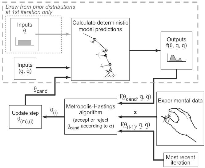
Open-loop structure of Monte Carlo simulations is enclosed by the gray dashed line. Note that Monte Carlo simulations always draw from the prior distributions, while MCMC simulations draw only from the prior distributions at the first iteration. All subsequent MCMC candidate parameter sets are perturbations of the most recent parameter sets. MCMC simulations directly compare model predictions and experimental data in a closed-loop manner. We built our Markov chains using a Metropolis–Hastings algorithm and single-site updating (see Section II-A for details on the notation).

Unfortunately, a severe limitation of Monte Carlo methods is that their computational demands grow exponentially with the number of model parameters [16]. When the number of parameters is large and/or each iteration is computationally expensive, such open-loop methods become computationally prohibitive. However, we can improve the efficiency of the simulations using advanced stochastic methods. One approach is to make the stochastic search data driven (or “closed loop”) by drawing dependent sets of parameters randomly from proposal distributions, feeding them through deterministic equations to predict system behavior, and comparing the predictions to experimental observations in a feedback manner (see Fig. 1). As a result, such data-driven MCMC sampling is biased toward parameter values that lead to model predictions that best agree with experimental data in a least-squares sense [17] (see Appendix A).

While Monte Carlo methods have been applied to biomechanical model parameter spaces ranging from 4 [14] to 50 dimensions [1], the use of MCMC methods has not been demonstrated for realistically large biomechanical models. To our knowledge, MCMC methods have only been used to match 3-D models of the human body to markerless motion capture data [18] and estimate neural activity from biosignals [19]–[21]. In this paper, we use synthetic data from a model of the human thumb as a proof-of-concept of an MCMC Metropolis–Hastings algorithm to explore a complex 36-D model parameter space and improve the fitness of the model. In addition, we explicitly investigate the effects of parameter variability and uncertainty on biomechanical model performance.

II. Methods

Using a truth model approach, we arbitrarily defined model parameters for a 5-DOF kinematic model of the thumb. We then generated synthetic, noisy kinematic output data for this model. Ten independent Markov chains [22] driven by these noisy data searched the model parameter space, which we systematically expanded from 3 to 8, 24, and 36 dimensions, for the subspace that best fit the data. We constructed chains with a Metropolis–Hastings sampling algorithm [23]–[25] on dual INTEL XEON, 2.4-GHz machines. We developed custom C code using the GNU Scientific Library [26], the MICROSOFT Visual Studio .NET Development Environment 2003, and the INTEL C++ Compiler 9.0. We performed the postanalysis in MATLAB 7.1 for visualization purposes.

Our prior work on Monte Carlo simulations of an anatomy-based model of the thumb [27]–[29] employed open-loop simulations and used experimental data to establish prior distributions, but did not use experimental data as a means to effectively explore the parameter space [2]. In this paper, we apply closed-loop MCMC simulations to the same model structure with nonorthogonal and nonintersecting axes of rotation and add model parameters to relate the model to surface marker experimental data. Thus, the model has 36 independent parameters (8 bone dimensions [30], 16 axes of rotation parameters [27]–[29], and 12 coordinate transformation parameters [31]) summarized by θ (see Fig. 2). The input variables to the 5-DOF serial linkage model are joint angles q and joint angular velocities q̇ representative of unimpaired kinematic behavior [31]. The output variables obtained deterministically from the serial linkage model are 3-D thumbnail location, orientation, linear velocities, and angular velocities.

Fig. 2.

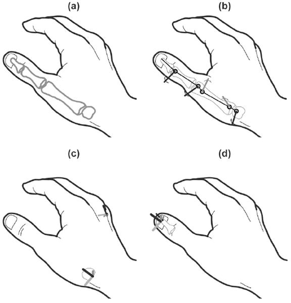
(a) Model structure consists of 36 independent model parameters: 8 bone dimensions [30], (b) 16 axes of rotation parameters [27]–[29], and (c), (d) 12 coordinate transformation parameters [31]. One transformation relates the proximal end of the thumb at the base of the trapezium to a space-fixed coordinate system on the back of the hand, while the other relates the distal end of the thumb at the tip of the distal phalanx to a body-fixed coordinate system on the thumbnail.

The experimental data matrix X is composed of n rows of observations × k = 13 columns of kinematic outputs. The jth observation makes up the jth row of data matrix X, whose individual elements are represented by x_j,k. Three-dimensional thumbnail location (x, y, z), orientation (expressed by four quaternion parameters q₀, q₁, q₂, q₃ [32], [33]), and linear velocity (ẋ, ẏ, ż) are expressed in F_fixed, a fixed global reference frame whose origin is located on the dorsum of the hand just proximal to the distal tip of the third metacarpal [Fig. 2(c)]. Angular velocity (ω′_x, ω′_y, ω′_z) is expressed in F_thumbnail, a local reference frame whose origin is located in the center of the thumbnail [Fig. 2(d)]. For both F_fixed and F_thumbnail, the (+)x-, y-, and z-axes point palmarly, radially, and distally, respectively

$${\underset{¯}{\mathbf{X}}}_j={[xyz{q}_0{q}_1{q}_3\dot{x}\dot{y}\dot{z}{\omega }_x^{\prime }{\omega }_y^{\prime }{\omega }_z^{\prime }]}_j.$$ (1)

A. Constructing Markov Chains Using Metropolis–Hastings Sampling Scheme

Ideally, we would know our target distribution π(θ) (the posterior distribution p(θ∣X), or the probability of the model parameter set θ given observed data X) and it would be a simple analytical expression or easy to sample from directly. When this is not the case, we can still estimate the target distribution by sampling from a stationary distribution π*(θ) that is proportional to the target distribution π(θ) and draw inferences on these results. We can estimate the expectation of any function of θ using averages of samples drawn after convergence to the stationary distribution.

The key to the MCMC approach is the use of an appropriate sampling scheme to construct ergodic Markov chains that converge to such a stationary distribution. If run long enough, these chains will locate and forever sample from a stationary distribution whose existence and uniqueness is guaranteed [34] and is our posterior distribution of interest by design. With the Metropolis–Hastings algorithm, we build ergodic chains by drawing each candidate parameter set θ_cand from a proposal distribution q(θ_cand∣θ_(i−1)) and accepting θ_cand with an acceptance probability α as per [23]–[25]

$$\alpha ({\underset{¯}{\theta }}_{\mathrm{cand}},{\underset{¯}{\theta }}_{(i-1)})=\min \left\{\frac{\pi ({\underset{¯}{\theta }}_{\mathrm{cand}})q({\underset{¯}{\theta }}_{(i-1)}\mid {\underset{¯}{\theta }}_{\mathrm{cand}})}{\pi ({\underset{¯}{\theta }}_{(i-1)})q({\underset{¯}{\theta }}_{\mathrm{cand}}\mid {\underset{¯}{\theta }}_{(i-1)})},1\right\}.$$ (2)

At each iteration, if a randomly drawn uniform variable U (0, 1) lies in the [0, α] range, we accept θ_cand and set θ_(i) = θ_cand. Otherwise, we reject θ_cand and set θ_(i) = θ_{(i − 1)}.

1) Prior Distributions

Boundaries on the prior distributions p(θ) can be set to known physiologically limited ranges (e.g., minimum/maximum bone length). Certainty or uncertainty can be represented by using distributions having small or large variances, respectively. We created bounds (mean ± standard derivation) for our conservative, noninformative, uniform prior distributions using sparse published [27]–[29] and measured data [30], [31]. Inappropriate selection of prior distribution bounds may exclude regions of the model parameter space where the posterior distribution actually resides. However, the shape of the prior distributions is not that critical due to the memoryless nature of the Markov chains. If run long enough, the chains will eventually converge to the distribution of interest regardless of “poor” initial conditions.

2) Proposal Distributions

The initial candidate parameter set θ_cand, the starting point of the chain, is drawn randomly from the prior distributions (see Fig. 1). The remaining θ_cand are perturbations of the most recent parameter set θ_{(i − 1)} by a “jump width” vector c whose elements are independently scaled by a uniform random variable u ~ i.i.d. ¹ U (0, 1) [35] for p = 1, …, d_param, the dimensionality of the model parameter space

$${\theta }_{p,\mathrm{cand},\mathrm{temp}}={\theta }_{p,(i-1)}\pm (c_p{u}_p).$$ (3)

Each c element is first arbitrarily set to 0.1% of each parameter’s allowable range. To gauge search efficiency, we calculate the acceptance rate as the percent of the total iterations that we accept θ_cand. High and low rates mean that the chain is “wandering” excessively (need to increase c) or “stuck” (need to decrease c), respectively. While convergence is guaranteed by ergodicity regardless of the acceptance rate, we adjust c automatically to achieve rates between 30% and 70% for each model parameter to minimize computing time [36]. We use a reflection technique [37] to ensure that all proposed model parameters remain within the prior distribution boundaries (LB_p, UB_p)

$${\theta }_{p,\mathrm{cand}}:=\{\begin{array}{ll}2{\mathrm{LB}}_p+c_p{u}_p-{\theta }_p,(i-1),& \mathrm{if}{\theta }_{p,\mathrm{cand},\mathrm{temp}}<{\mathrm{LB}}_p\\ 2{\mathrm{UB}}_p-c_p{u}_p-{\theta }_p,(i-1),& \mathrm{if}{\theta }_{p,\mathrm{cand},\mathrm{temp}}>{\mathrm{UB}}_p\\ {\theta }_{p,\mathrm{cand},\mathrm{temp},}& \mathrm{otherwise}.\end{array}$$ (4)

3) Likelihood Function

The likelihood function p(X∣θ) is the probability of observing data X given the model parameter set θ. For our likelihood function, we assume that the experimental data matrix X is composed of n i.i.d. observations. We assume that each observation X_j [the jth row of data matrix X, (1)] is i.i.d. from a multivariate Gaussian distribution MVN (f(θ), Σ̂), with a vector of means f(θ) that is a deterministic function of θ and a covariance matrix $\widehat{\sum }=\mathrm{diag}({\widehat{\sigma }}_k^2)$ where k = 1, …, d_expt, the dimensionality of the experimental measurements (number of columns in X).

At each iteration, we estimate ${\widehat{\sigma }}_k^2$ as the sum of the squared residuals divided by a random variable from a χ²-distribution with (n – 1) DOF. The variance estimates are affected by both measurement uncertainty in X_j and modeling errors in f_pred (θ_(i), q_j, q̇_j), where q_j and q̇_j represent the constant input joint angles and joint angular velocities for the jth observation

$${\widehat{\sigma }}_k^2=\frac{{\sum }_{j=1}^n{[x_{j,k}-f_k(\underset{¯}{\theta },{\underset{¯}{q}}_j,{\dot{\underset{¯}{q}}}_j)]}^2}{{\chi }_{(n-1)}^2}.$$ (5)

After applying these assumptions and simplifying (see Appendix A), we are left with the following acceptance probability equation (6), as shown at the bottom of the page. If θ_cand does not predict the experimental data matrix X well, α is small and θ_cand is less likely to be accepted.

4) Updating Scheme

The probability of proposing and accepting a “jump” from one point in our high-dimensional parameter space to an entirely unrelated point in the space is very low. Thus, we adopt the “single-site” updating scheme, or “single-component Metropolis–Hastings,” in which one element of the model parameter set is varied at a time [37]. For each iteration i, we perform an update step m for each dimension in the model parameter space (e.g., m = 36 update steps for the 36-D space of test case 6). At the first update step, we perturb the first element of θ_cand [via (3)], shown here for the 36-D test case

$$\alpha ({\underset{¯}{\theta }}_{\mathrm{cand}},{\underset{¯}{\theta }}_{(i-1)})=\min \left\{\frac{\exp \left\{-(1/2){\sum }_{k=1}^{d_{\mathrm{expt}}}{\sum }_{j=1}^n{[x_{j,k}-f_k({\underset{¯}{\theta }}_{\mathrm{cand}},{\underset{¯}{q}}_j,{\dot{\underset{¯}{q}}}_j)]}^2/{\widehat{\sigma }}_k^2{,}_{(i-1)}\right\}}{\exp \left\{-(1/2){\sum }_{k=1}^{d_{\mathrm{expt}}}{\sum }_{j=1}^n{[x_{j,k}-f_k({\underset{¯}{\theta }}_{(i-1)},{\underset{¯}{q}}_j,{\dot{\underset{¯}{q}}}_j)]}^2/{\widehat{\sigma }}_k^2{,}_{(i-1)}\right\}},1\right\}$$ (6)

$${\underset{¯}{\theta }}_{\mathrm{cand},(m=1),(i)}=\left[\begin{array}{c}{\theta }_{1,\mathrm{cand}}\\ {\theta }_{2,(i-1)}\\ ⋮\\ {\theta }_{36,(i-1)}\end{array}\right].$$ (7)

We calculate the acceptance probability and either accept (θ_1,(i) = θ_1,cand) or reject (θ_1,(i) = θ_1,(i−1)) the element θ_1,cand. At the second update step, we perturb the second element θ_2,cand and so on

$${\underset{¯}{\theta }}_{\mathrm{cand},(m=2),(i)}=\left[\begin{array}{c}{\theta }_{1,(i)}\\ {\theta }_{2,\mathrm{cand}}\\ {\theta }_{3,(i-1)}\\ ⋮\\ {\theta }_{36,(i-1)}\end{array}\right].$$ (8)

B. Post Hoc Analysis

1) Assessing Convergence of MCMC Simulations

MCMC being a stochastic process, there is no analytical expression for predicting a sufficient number of iterations prior to running the simulations. Thus, we run diagnostics on MCMC simulation outputs in a post hoc manner. We use the Gelman–Rubin convergence diagnostic $\sqrt{\widehat{R}}$ [38], [39] to assess convergence because it is an empirical metric that is recommended for use with multiple chains. Briefly, $\sqrt{\widehat{R}}$compares the variance among independent Markov chains to the variance within each chain [22], [36], [37] and approaches one as the independent chains converge to and sample from the same stationary distribution. In practice, we want $\sqrt{\widehat{R}}$ to permanently fall below a threshold (1.2, per [39]) for all input and output scalars of interest, as this indicates convergence. The iterations preceding the crossing of the $\sqrt{\widehat{R}}$threshold are discarded as part of the burn-in period.

The iterations after the burn-in period are often thinned according to a user-specified thinning interval p to reduce costs such as computational storage and postanalysis time [22], [39]. Every pth iteration of each chain is selected and pooled. The model parameter set at each of these pooled iterations is a draw from the joint posteriors and can be used to draw inferences about the model. We know of no widely accepted number of converged iterations necessary for adequate sampling of the posterior distribution, but due to the law of large numbers [40], many iterations beyond convergence will only serve to refine the distribution. We arbitrarily extended chains to obtain 25 000 converged iterations per chain, thus ensuring 1000 thinned iterations with p = 25.

2) Posterior Predictive Sampling

To obtain posterior predictive samples f_pred,noisy (θ_(i), q_j, q̇_j) that account for measurement noise, we add zero-mean, uncorrelated multivariate Gaussian noise [ ${\widehat{\sum }}_{(i)}=\mathrm{diag}({\widehat{\sigma }}_{(i)}^2)$; (5)] to the deterministic model predictions f_pred (θ_(i), q_j, q̇_j)

$$f_{\mathrm{pred},\mathrm{noisy}}({\underset{¯}{\theta }}_{(i)},{\underset{¯}{q}}_j,{\dot{\underset{¯}{q}}}_j)=f_{\mathrm{pred}}({\underset{¯}{\theta }}_{(i)},{\underset{¯}{q}}_j,{\dot{\underset{¯}{q}}}_j)+\mathrm{MV}N(\underset{¯}{0},{\widehat{\sum }}_{(i)}).$$ (9)

The distributions of the posterior predictive samples (over all thinned, converged iterations) are then compared to each inherently noisy experimental observation X_j.

3) Cross-Validating the Model

Posterior predictive sampling indicates how well the joint posteriors can predict the experimental data provided to the Metropolis–Hastings algorithm. However, model cross validation must be performed using a separate set of experimental observations X_val not provided to the algorithm. Cross validation is identical to posterior predictive sampling except that each joint posterior draw θ_(i) is used to predict model outputs under different conditions (i.e., different joint angles q and joint angular velocities q̇). The variance estimates are recalculated [see (5)] and noise is added [see (9)] prior to comparison with X_val.

C. Validating Sampling Algorithm Using Truth Model “Test Cases”

Truth models are used to validate algorithms because the researcher defines the model structure, its parameter values, and its deterministic behavior, and focuses on the algorithm’s performance itself. In this paper, we defined a “virtual subject” having a true model parameter set θ_true and model inputs (joint angles q and joint angular velocities q̇). We calculated the deterministic model outputs f(θ_true, q, q̇), which were necessarily free of measurement noise. We added simulated zero-mean, uncorrelated multivariate Gaussian “measurement noise” MV N (0, Σ̂_true) to our deterministic model outputs f(θ_true, q, q̇) and treated the noisy results f (θ_true,noisy, q, q̇) as experimental data, similar to our posterior predictive methods [see (9)]. For convenience, we defined ${\widehat{\sum }}_{\mathrm{true}}=\mathrm{diag}({\widehat{\sigma }}_{k,\mathrm{true}}^2)$. We used these simulated “noisy” experimental data to drive our MCMC simulations

$$f({\underset{¯}{\theta }}_{\mathrm{true},\mathrm{noisy}},\underset{¯}{q},\dot{\underset{¯}{q}})=f({\underset{¯}{\theta }}_{\mathrm{true}},\underset{¯}{q},\dot{\underset{¯}{q}})+\mathrm{MV}N(\underset{¯}{0},{\widehat{\sum }}_{\mathrm{true}}).$$ (10)

Due to the high-dimensional nature of the parameter space and the fact that we were developing custom C code, we worked through a series of truth model “test cases” to validate our algorithm (see Fig. 3 and Table I).Test cases 1–3 used three free parameters only, requiring a search of a 3-D parameter space. Test cases 1 and 2 were planar and 3-D kinematic models of the thumb, respectively, with orthogonal and intersecting axes of rotation. Test case 3 was a trivial upgrade to test case 2 that used different constants for the axes of rotation model parameters to simulate a kinematic model of the thumb based on the “virtual five-link model” with nonorthogonal and nonintersecting axes of rotation (Table I). Once the sampling scheme worked for these three test cases, we systematically increased the dimensionality of the parameter space from 3 to 8, 24, and 36. Test case 6, with the 36-D parameter space, is the level of complexity we are truly interested in for practical application to experimental data.

Fig. 3.

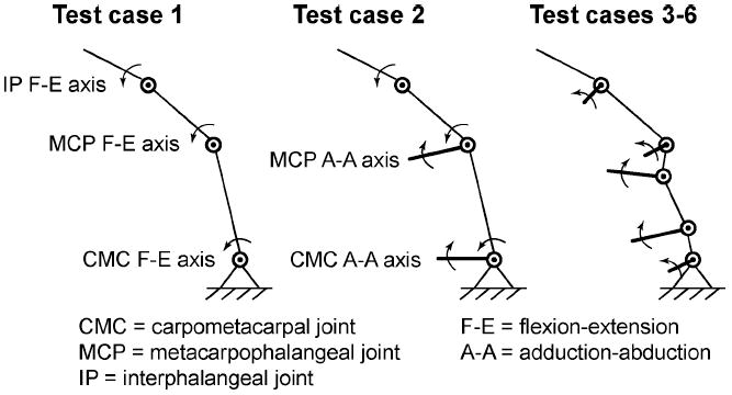
Truth model test cases used for the validation of our Metropolis–Hastings sampling algorithm are shown. From left to right, the models were assigned 3, 3, and (3, 8, 24, and 36) free model parameter values, respectively (see Table I).

Table I.

Six Truth Model Test Cases Were Used to Validate Our Metropolis–Hastings Sampling Algorithm (See Fig. 3)

		Test case		1	2	3	4	5	6
		Dimensionality of model parameter space		3	3	3	8	24	36
		Rotational degrees of freedom		3	5
		Axes of rotation		orthogonal, intersecting		non-orthogonal, non-intersecting
Parameters for bone dimensions	1	metaz	Distal length of metacarpal	-	-	-	-	-	-
	2	metaratx	Palmar/distal length for metacarpal	0.3402	0.3402	0.3402	-	-	-
	3	metaraty	Radial/distal length for metacarpal	0.3602	0.3602	0.3602	-	-	-
	4	proxphalz	Distal length of proximal phalanx	-	-	-	-	-	-
	5	proxratx	Palmar/distal length for proximal phal.	0.4176	0.4176	0.4176	-	-	-
	6	distphalz	Distal length of distal phalanx	-	-	-	-	-	-
	7	trapratz	Trapezium/proximal phalanx distal lengths	0	0	0	-	-	-
	8	trapratx	Palmar/distal length for trapezium	1.1855	1.1855	1.1855	-	-	-
Parameters specifying the location and orientation of the axes of rotation (orientation param. in rad.)	9	BETAcmcFE	Orientation parameter for CMC FE axis	0	0	0.1151	0.1151	-	-
	10	bpercCMCFE	Location parameter for CMC FE axis	0.5	0.5	0.347	0.347	-	-
	11	ALPHAcmcAA	Orientation parameter for CMC AA axis	1.5708	1.5708	1.4824	1.4824	-	-
	12	BETAcmcAA	Orientation parameter for CMC AA axis	1.5708	1.5708	1.2027	1.2027	-	-
	13	tpercCMCAA	Location parameter for CMC AA axis	0.5	0.5	0.5573	0.5573	-	-
	14	IpercCMCAA	Location parameter for CMC AA axis	0	0	0.1586	0.1586	-	-
	15	ALPHAmpAA	Orientation parameter for MP AA axis	1.5708	1.5708	1.4099	1.4099	-	-
	16	BETAmpAA	Orientation parameter for MP AA axis	1.5708	1.5708	1.3123	1.3123	-	-
	17	tpercMPAA	Location parameter for MP AA axis	0.5	0.5	0.4792	0.4792	-	-
	18	IpercMPAA	Location parameter for MP AA axis	1	1	0.8617	0.8617	-	-
	19	ALPHAmpFE	Orientation parameter for MP FE axis	1.5708	1.5708	1.8289	1.8289	-	-
	20	tpercMPFE	Location parameter for MP FE axis	0.5	0.5	0.6425	0.6425	-	-
	21	IpercMPFE	Location parameter for MP FE axis	1	1	0.835	0.835	-	-
	22	BETAipFE	Orientation parameter for IP FE axis	1.5708	1.5708	1.4265	1.4265	-	-
	23	tperclPFE	Location parameter for IP FE axis	0.5	0.5	0.5918	0.5918	-	-
	24	IperclPFE	Location parameter for IP FE axis	1	1	0.9036	0.9036	-	-
Parameters for 3D frame transform. at the proximal base (FF) and distal tip (FN) of the thumb	25	FF_rotz	Euler rot. ang. about z-axis for FF frame	0	0	0	0	0	-
	26	FF_roty	Euler rot. ang. about y-axis for FF frame	0	0	0	0	0	-
	27	FF_rotx	Euler rot. ang. about x-axis for FF frame	0	0	0	0	0	-
	28	FF_trx	Translation along x-axis for FF frame	0	0	0	0	0	-
	29	FF_try	Translation along y-axis for FF frame	0	0	0	0	0	-
	30	FF_trz	Translation along z-axis for FF frame	0	0	0	0	0	-
	31	FN_rotz	Euler rot. ang. about z-axis for FN frame	0	0	0	0	0	-
	32	FN_roty	Euler rot. ang. about y-axis for FN frame	0	0	0	0	0	-
	33	FN_rotx	Euler rot. ang. about x-axis for FN frame	0	0	0	0	0	-
	34	FN_trx	Translation along x-axis for FN frame	0	0	0	0	0	-
	35	FN_try	Translation along y-axis for FN frame	0	0	0	0	0	-
	36	FN_trz	Translation along z-axis for FN frame	0	0	0	0	0	-

Boxes with dashes indicate free variables that make up the model parameter space.

III. Results

Despite the high-dimensional model parameter space, the MCMC simulations converged, and the joint posterior distribution for all model parameters was obtained for test cases ranging from 3 to 36 dimensions. As expected, the burn-in period increased as the dimensionality of the model parameter space increased (Table II). The true posterior distribution for the 3-D test case 3 was found quickly, while the 36-D test case 6 took much longer (burn-in iterations of 919 and 56 400, respectively). The Markov chains also found more local minima as the dimensionality of the model parameter space increased. All ten chains settled on a single minima (true posterior) for the 3-D and 8-D test cases. The ten chains located two and four local minima (including the true posterior) for the 24-D and 36-D test cases, respectively.

Table II.

Summary of MCMC Convergence Statistics Is Shown for Six Truth Model Test Cases

Test case	Dim. of param. space	Total iter. per chain	Burn-in iter.	# of chains to find true posterior (out of 10)	Converged iter. after thinninga	# of minima found thus far
1	3	4,005	455	10	1,420	1 (true)
2	3	3,005	480	10	1,010	1 (true)
3	3	3,020	919	10	840	1 (true)
4	8	4,025	1,600	10	970	1 (true)
5	24	25,000	13,841	8	3,570	2 (inc. true)
6	36	105,000	56,400	6	11,664	4 (inc. true)

We used a thinning interval of 25 iterations.

Not surprisingly, our search of the 36-D test case 6 took the longest to converge likely due to the “curse of dimensionality” [16] as well as the potential for an increased number of local minima in the fitness landscape. For test case 6, we ran ten independent Markov chains of 105 000 iterations each on 2.4-GHz dual INTEL XEON machines, which took 255.5 h (49 h for MCMC simulations in C and 206.5 h for postanalysis in MATLAB 7.1), or approximately 10.6 days of wall clock time.

For the 36-D model parameter space, the time history of the sum of the squared residuals between the model predictions and the simulated experimental data [numerator of (5)] showed that a six-chain subset (majority of the ten independent chains) had sums of squared residuals that were two orders of magnitude smaller than the next best-performing chain. Upon further inspection, it was found that this six-chain subset had converged to the true posterior distribution, while the remaining four chains (a single two-chain subset and two individual chains) found other local minima in the 36-D landscape (see Fig. 4). In all, four distinct types of behavior were observed after convergence.

Fig. 4.

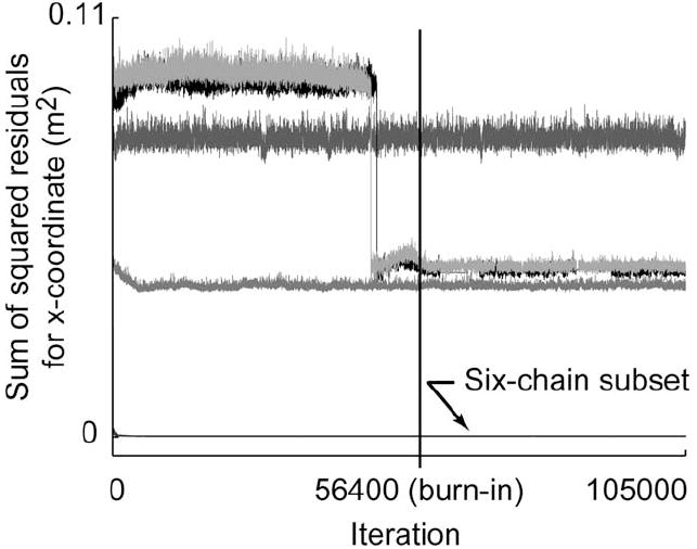
Time history of the sum of the squared residuals [summed across all data points, see numerator of (5)] is shown for a representative model output (thumbnail x-coordinate) for the 36-D test case 6. Each trace corresponds to the performance of a single Markov chain. The burn-in iteration is represented by the vertical line at iteration 56 400. The six-chain subset that located the true posterior distribution had values on the order of 2E–4m². Four other chains had larger residuals ranging from 4E–2 to 8E–2m², suggesting that they had found local minima.

When including all ten Markov chains for the 36-D test case 6, the Gelman–Rubin convergence diagnostic failed to converge to values below our threshold of 1.2. By restricting the $\sqrt{\widehat{R}}$ calculations to the six-chain subset, we determined a burn-in period of 56 400 iterations (see Fig. 5). At this point, each of the six independent chains had located the true posterior distribution and were sampling from the same region of the model parameter space despite their overdispersed initial conditions.

Fig. 5.

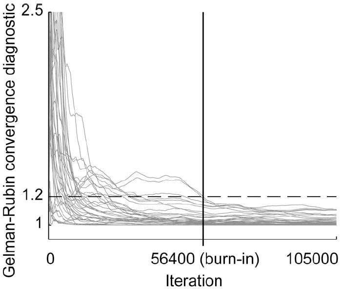
For the best-performing six-chain subset from the 36-D test case 6, the Gelman–Rubin convergence diagnostic values $\sqrt{\widehat{R}}$ satisfied our threshold of 1.2 (dashed line) by a burn-in iteration of 56 400 (vertical line).

For the 36-D test case 6, the first 7500 iterations are shown for two representative model parameters in Fig. 6(a). This subplot illustrates the overdispersed initial conditions of the ten Markov chains, exploration of the parameter space, and the movement of some of the chains toward the true posterior distribution. Note that an open-loop Monte Carlo integrator must randomly sample from the entire volume to achieve convergence. Fig. 6(b) shows the burn-in iterations as well as samples from the true posterior for three representative model parameters. While only 3-D results are shown, convergence occurred in 36-D for this test case 6, making the efficiency of the MCMC approach all the more striking. It is clear that independent chains are able to converge to the appropriate region of the high-dimensional parameter space without the computationally prohibitive exploration of every point in the 36-D space.

Fig. 6.

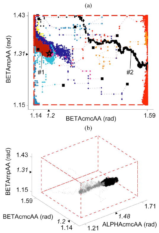
(a) Overdispersed initial conditions (solid squares) for ten independent Markov chains are shown for two representative parameters for the 36-D test case 6. Some chains (e.g., 1) located the true posterior (true parameter values marked by a star), while others (e.g., 2) found local minima. (b) History of the six-chain subset is shown for three representative parameters for the 36-D test case 6. Burn-in and pooled converged iterations are shown in gray and black, respectively. For both (a) and (b), prior distribution bounds are represented by dashed lines, and tick marks and triangles on the axes indicate the parameter bounds and true values, respectively.

From our thinned, converged posterior distribution draws, we immediately have the probability density function for each element of θ, also called the marginal distribution. The marginal distributions for the 3-D test case 3 are sharp and have tight ranges [Fig. 7(a), (d), and (f)]. With only three free model parameters, there are relatively few parameter combinations that lead to model predictions that agree well with the simulated experimental observations. In contrast, the marginal distributions for the 36-D test case 6 varied in breadth (Figs. 7-9). Of the eight bone parameters, the longitudinal lengths of the thumb bones appeared to be the most important for predicting the simulated kinematic experimental data.

Fig. 7.

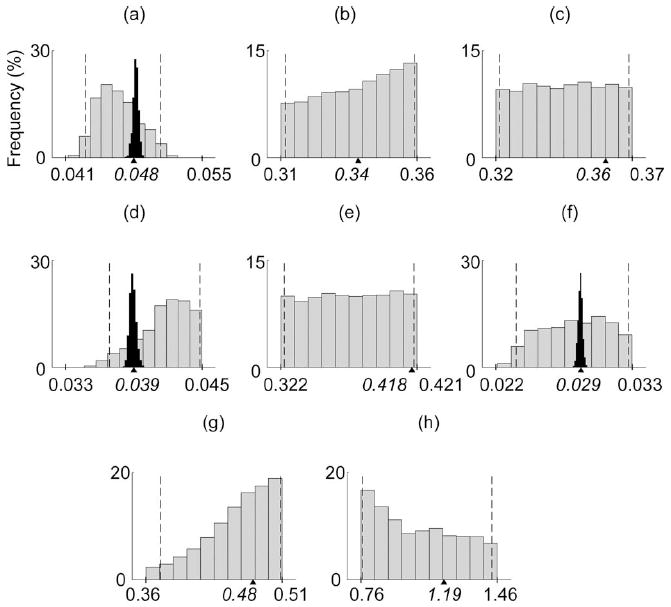
Marginal distributions are shown for the eight bone parameters [30] for the 36-D test case 6 (gray bars) and the 3-D test case 3 [black bars in (a), (d), and (f)]. Dashed lines indicate the 95% confidence intervals (for the 36-D test case 6), while tick marks and triangles on the x-axes indicate the parameter bounds and true values, respectively.

Fig. 9.

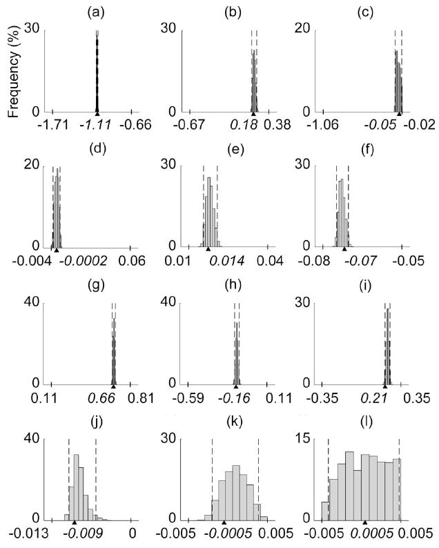
Marginal distributions are shown for the 12 parameters for the frame transformations at the proximal base and distal tip of the thumb [31] for the 36-D test case 6. Dashed lines indicate the 95% confidence intervals, while tick marks and triangles on the x-axes indicate the parameter bounds and true values, respectively.

Of the 16 axes of rotation model parameters, those specifying the orientation of the most proximal joint axes (e.g., BETAcmcAA) had the most narrow marginal distributions, suggesting their importance in the model (see Fig. 8). Almost all model parameters associated with the 3-D frame transformations at the proximal base and distal tip of the thumb had extremely sharp marginal distributions, highlighting the sensitivity of the model to these parameters (see Fig. 9).

Fig. 8.

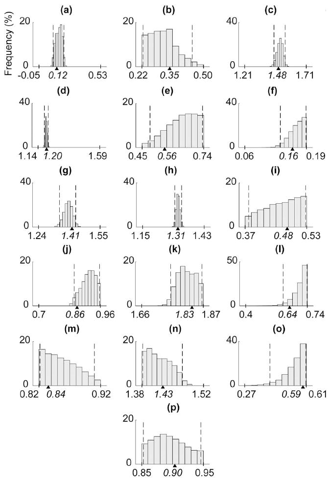
Marginal distributions are shown for the 16 axes of rotation parameters [27]–[29] for the 36-D test case 6. Dashed lines indicate the 95% confidence intervals, while tick marks and triangles on the x-axes indicate the parameter bounds and true values, respectively.

For the 36-D test case 6, the errors in the posterior predictive samples for the six chains were minimal [Fig. 10(a) and (b)]. Despite the noise in the simulated data [see (10)], the Metropolis–Hastings algorithm was able to estimate and account for the simulated measurement errors that we added to the “clean” deterministic truth model outputs to successfully locate the true posterior distribution. The errors in the posterior predictions for the cross-validation dataset were also minimal [Fig. 10(c) and (d)], demonstrating that the algorithm did not simply overfit the data given, but actually found the true parameters in the 36-D space.

Fig. 10.

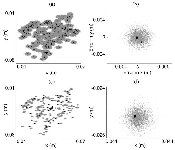
Posterior prediction [(a) and (b)] and cross-validation [(c) and (d)] results are shown for the 36-D test case 6 for two experimental outputs: x and y thumbnail coordinates. (a) Posterior predictive samples (gray points) are clustered around the true model outputs (solid circles) despite the use of noisy data [open circles; see (10)]. (b) Posterior predictive sample errors are shown for a single data point [see box in (a)]. The solid and open circles indicate the true error value of zero and offset of the noisy simulated data point, respectively. (c) Model predictions (gray points) are clustered around the cross-validation data (solid circles). (d) Close-up view of a single data point [see box in (c)] is shown.

IV. Discussion

We have demonstrated a proof-of-concept for our Metropolis–Hastings sampling algorithm for a complex 36-D model parameter space with practical application to experimental data. Contrary to the assumed notion that MCMC methods are computationally prohibitive for nontrivial models, we have shown the feasibility of MCMC methods to improve the fitness of biomechanical models with large numbers of parameters. The advantages, limitations, implications, and applications of this paper are described here.

A. Foundation for Bayesian Approach

MCMC methodology is often criticized for its subjective selection of the prior distribution. However, proponents of the Bayesian philosophy counter that: 1) prior information should be used if available [22]; 2) if the MCMC simulations are run to convergence, the use of possibly naïve prior distributions becomes less important as the data “speak for themselves” [22], [36]; and 3) the subjective selection of the prior distribution is no different from the a priori subjective selection of a likelihood function for maximum likelihood estimation [22].

The Bayesian viewpoint is particularly appropriate for biomechanical modeling, where anatomical variability is the rule, because each parameter has its own probability distribution. A frequentist approach yields a single set (point estimate) of model parameters that optimizes some objective function [41]. In contrast, a Bayesian approach such as MCMC yields distributions (cloud estimates) of model parameters and their outputs that have been informed by experimental data [37]. With distributions, revealing properties are immediately available: probability densities, parameter ranges, skewness, kurtosis, and multimodality. Confidence intervals and means are trivial to extract. Furthermore, the parameter marginal distributions that result can be used as informative prior distributions for future simulations, instead of the diffuse priors used at the start of such parameter estimation processes.

MCMC simulations are essentially stochastic, data-driven sensitivity analyses that enable us to determine the effects of parameter variability and uncertainty resulting from natural anatomical variability across a population and sparseness of experimental data, respectively. Latent parameter covariances that may not have been explicitly measured (and may not be measurable) can be extracted from the joint posterior, justifying a reduction in model complexity.

B. Effects of Increasing Parameter Space Complexity

During the validation of our Metropolis–Hastings algorithm, we gradually increased the dimensionality of the model parameter space from 3 to 8, 24, and 36 dimensions (Table I). As expected, convergence time (Table II) increased with the complexity of the model parameter space.

When landscape complexity increased, an increasing number of independent Markov chains located local minima. All ten Markov chains successfully located the true posterior distribution for the 3-D and 8-D scenarios (test cases 3 and 4, respectively). However, the number of chains to wander into local minima were two and four for the 24-D and 36-D scenarios (test cases 5 and 6, respectively). Importantly, in all cases, the majority of the Markov chains successfully located the true posterior distribution. In theory [34], “trapped” chains should eventually “escape” local minima if run long enough. However, due to the stochastic nature of the sampling method, we cannot determine how long convergence will take a priori.

Guided by our Gelman–Rubin convergence diagnostic, we pooled the majority of the chains that converged and found that they had indeed located the true posterior distribution. As the complexity of the model parameter space increased, we found that the marginal distributions became more varied in range and shape (described shortly).

C. Marginal Distributions

The model parameter marginal distributions (Figs. 7-9) provide insight into the sensitivity of the model predictions to variability in the model parameters. A sharp marginal distribution [e.g., Fig. 8(d)] suggests high sensitivity of the model predictions to variation in the parameter, while a flat marginal distribution [e.g., Fig. 7(c)] can be due to a variety of reasons. The simplest reason is insensitivity of model predictions to variations in the parameter because the parameter values do not affect the model output [13], [42]. In this case, the parameter could be set to a constant and removed from the model parameter space altogether, thereby reducing the dimensionality of the parameter space and the number of update steps per iteration.

There could also be redundancy in the model structure itself. The flattest marginal distributions we observed were for model parameters that relate bone widths and lengths [Fig. 7(c) and (e)]. In our model structure, we represent bones by their bounding box dimensions. It may be that a “link” in our serial linkage model could fit within this bounding box in a variety of ways (e.g., perfectly aligned within the box or more diagonally oriented within the box). This redundancy could allow for greater variance of the model parameters that relate bone widths and lengths, but less variance in the model predictions. Finally, the flat marginal distributions could result from unobservability [41] because effects of the model parameters cannot be observed within the experimental data.

The range of the marginal distributions can highlight a need to reassess the prior distribution bounds. For instance, a marginal distribution that is pushed up against a parameter’s upper bound [e.g., Fig. 7(g)] may suggest a need to reevaluate the appropriateness of the bound. If the bound is nonnegotiable, then the MCMC results point directly to limiting aspects of the model structure.

It is interesting that the marginal distributions for the 3-D test case 3 had tight ranges and sharp distributions as compared to their counterparts for the 36-D test case 6 [Fig. 7(a), (d), and (f)]. This was not expected a priori. However, these results are not unreasonable given the increased chance of observing the effects of parameter insensitivity, model redundancy, and unobservability as the complexity of the model parameter space increases.

D. Correlations Among Bone Lengths

From an anatomical perspective, it is reasonable to expect that larger people have larger hands and that bone lengths scale up, resulting in a positive correlation among bone lengths. However, this issue concerns trends across a population and cannot be addressed by the truth model in this study, which focused on modeling a single virtual subject. To ensure proper sampling of the parameter space within our single-site updating scheme, we removed constraints on relative bone lengths and allowed bone dimensions to be drawn independently of the others. While this does not explicitly enforce physiological realism, it ensures that our Metropolis–Hastings algorithm is properly constructed such that convergence to the posterior distribution is guaranteed. Simulation results can be checked easily for physiologically realistic relationships upon convergence. In addition, “block-updating” can be used to incorporate such parameter correlations and improve the efficiency of the search [37], [43]. With block updating, correlated model parameters are perturbed as a subset rather than individually, as with single-component Metropolis–Hastings. For instance, let model parameters 1–3 be correlated. At the first update step (m = 1), we perturb the first three parameters as a block. At the second update step, we continue the single-site updating from the 4th parameter, shown here for the 36-D test case

$${\underset{¯}{\theta }}_{\mathrm{cand},(m=1),(i)}=\left[\begin{array}{c}\left[\begin{array}{c}{\theta }_{1,\mathrm{cand}}\\ {\theta }_{2,\mathrm{cand}}\\ {\theta }_{3,\mathrm{cand}}\end{array}\right]\\ {\theta }_{4,(i-1)}\\ ⋮\\ {\theta }_{36,(i-1)}\end{array}\right].$$ (11)

E. Gelman–Rubin Convergence Diagnostic

For the 36-D test case 6, $\sqrt{\widehat{R}}$ never fell below our threshold of 1.2 when calculating the shrink factor for all ten Markov chains together [Fig. 5(a)]. This apparent lack of convergence is not due to inadequacies of the MCMC approach, as has been successful in other applications [23], [44], including problems with 200 dimensions [45]. The lack of convergence likely results because we are exploring a complex, nonlinear landscape with multiple local minima, and by construction, $\sqrt{\widehat{R}}$ will not indicate convergence until all chains overlap in their sampling regions. Unfortunately, we have not found literature that explains how to deal with the failure of $\sqrt{\widehat{R}}$ for multimodal posterior distributions.

Nonetheless, $\sqrt{\widehat{R}}$ remains a popular, straightforward, and effective means to assess the progress of MCMC simulations. We took a common sense approach and calculated $\sqrt{\widehat{R}}$ for the six-chain subset that was obviously sampling from the same subspace and found that $\sqrt{\widehat{R}}$ satisfied our threshold [Fig. 5(b)].

F. Posterior Distribution Multimodality: Real or Artifact?

A valid concern with the MCMC approach is how to distinguish between modes that actually exist in a population and those that arise because of a complex high-dimensional model parameter space and/or the search methodology. With our truth model, we know that six of ten chains converged to the true posterior distributions, while four chains wandered into local minima (see Fig. 4). It may appear that we have found alternative solutions to the same problem, but further inspection reveals that the solutions are not equivalent and some outperform others (Fig. 4). If we had run a nonlinear least-squares optimization (a frequentist technique) and found two different solutions² (a likely occurrence given that convergence is also a challenge for these other methods), we would immediately look at the cost function for each solution and use the model that performs better. We could set a cost threshold relevant to the research question, objectively select the “best” mode, and use it to represent the true posterior distribution.

The “Achilles heel” of all search algorithms is that local minima can attract the algorithms to false solutions, often resulting in multimodal posterior distributions. Note that this only occurred for test cases 5 and 6, when the model parameter spaces were large (24-D and 36-D, respectively). One advanced technique for dealing with multimodality is Metropolis-coupled MCMC, or “hot-swapping” [46], [47], where one continuously monitors a user-defined metric [e.g., the sum of the squared residuals (Fig. 4)]. A chain that is presumably trapped in a local minimum is given an opportunity to swap one or more states (model parameter values) with a chain that has located a better performing region in parameter space. Using a process analogous to the genetic algorithm concepts of recombination and crossover [48], this swapping enables chains to escape from their local attractors.

G. Application to Clinical Questions

The Bayesian concept that “true” parameters are random variables is well suited to study how anatomical variability in musculoskeletal systems affects biomechanical function and contributes to the success or failure of a clinical method. The MCMC approach is not appropriate for quick subject-specific parameterizations (as in [49]) due to its computationally intensive nature. Rather, one can address whether a model structure will lead to meaningful clinical predictions. All too often, a model structure is assumed and its large-scale contributions to the success or failure of the model are overlooked and overshadowed by the need to specify its numerical details (i.e., the parameter estimation problem). With MCMC, the user can test a hypothesized model structure (e.g., anatomical kinematic constraints) against experimental data to elucidate the capabilities and limitations of such a structure [50].

The MCMC methods described here can be used to test whether a “one size fits all” model will suffice for the entire population, or if subject-specific models will be necessary. For instance, one can run separate sets of MCMC simulations each driven by various subsets of the experimental data. One could compare the posterior distributions from a group of subjects with presumably similar levels of impairment to those of a single member of that subpopulation.

The MCMC approach can highlight critical treatment-relevant model parameters and may be useful for defining clinically relevant subpopulations (e.g., different modes) for susceptibility to impairment and/or response to treatment. By tracking posterior distribution characteristics for a population of interest over time, it may be possible to observe the evolution of a disease state in model parameter space. Such insights could be used to devise objective methods of grading impairment. Strong correlations between easily measured model parameters and functional behavior could be incorporated into diagnostic tools. Furthermore, one can determine which model parameter(s) can afford to be noisy because of anatomical and/or surgical variability. We continue to address these issues to produce clinically useful models for studying the functional consequences of orthopedic and neurological diseases and treatments, and their treatment outcomes.

Biographies

Veronica J. Santos (M’03) received the B.S. degree in mechanical engineering with a music minor from the University of California, Berkeley, in 1999, and the M.S. and Ph.D. degrees in mechanical engineering with a biometry minor from Cornell University, Ithaca, NY, in 2004 and 2007, respectively.

From 2007 to 2008, she was a Postdoctoral Research Associate at the A. E. Mann Institute for Biomedical Engineering, University of Southern California, Los Angeles. She is currently an Assistant Professor in the Department of Mechanical and Aerospace Engineering, Arizona State University, Tempe. Her current research interests include hand biomechanics, neural control of movement, robotics, stochastic modeling, and clinical applications of biomechanical modeling for prosthetics and rehabilitation technology.

Prof. Santos is a member of the IEEE Engineering in Medicine and Biology Society, the American and International Societies of Biomechanics, the American Society of Mechanical Engineers, the Biomedical Engineering Society, the Society for the Neural Control of Movement, and the Society of Women Engineers. She was the recipient of the Young Investigator Poster Presentation Award from the International Society of Biomechanics (2005), an Exceptional Teaching Assistant Award from the Sibley School of Mechanical and Aerospace Engineering at Cornell University (2005), and a National Science Foundation Graduate Research Fellowship (2001).

Carlos D. Bustamante received the B.A. degree in biology, the M.S. degree in statistics, and the Ph.D. degree in biology from Harvard University, Cambridge, MA, in 1997 and 2001, respectively.

In 1998, he was a National Science Foundation Graduate Research Fellow. From 199 to 2000, he was a Howard Hughes Graduate Fellow. From 2001 to 2002, he was a Postdoctoral Fellow in the Mathematical Genetics Group of the Department of Statistics, University of Oxford, Oxford, U.K. He is currently an Associate Professor in the Department of Biological Statistics and Computational Biology and the Department of Statistical Sciences, Cornell University, Ithaca, NY, where he is also an Alfred P. Sloan Research Fellow in Molecular Biology. His current research interests include population genetics and genomics, statistical genetics and genomics, computational statistics, and application of Markov chain Monte Carlo techniques to problems in biology.

Prof. Bustamante is a member of the Society for Molecular Biology and Evolution and the American Society of Human Genetics. He has received various awards including a Marshall-Sherfield Fellowship to the University of Oxford, Oxford, U.K. He was the recipient of the Cornell Provost’s Award for Distinguished Research (2008).

Francisco J. Valero-Cuevas (M’99) received the B.S. degree in engineering from Swarthmore College, Swarthmore, PA, in 1988, and the M.S. degree in mechanical engineering from Queen’s University, Kingston, ON, Canada, in 1991, and the Ph.D. degree in mechanical engineering from Stanford University, Stanford, CA, in 1997.

He is currently an Associate Professor in the Department of Biomedical Engineering and the Division of Biokinesiology and Physical Therapy, University of Southern California, Los Angeles. His current research interests include combining engineering, robotics, mathematics and neuroscience to understand organismal, and robotic systems for basic science, engineering, and clinical applications.

Prof. Valero-Cuevas is a member of the IEEE Engineering in Medicine and Biology Society, the American and International Societies of Biomechanics, the American Society of Mechanical Engineers, the Society for Neuroscience, and the Society for the Neural Control of Movement. He was recipient of the Research Fellowships from the Alexander von Humboldt (2005) Foundation, the Postdoctoral Young Scientist Award from the American Society of Biomechanics (2003), the Faculty Early Career Development Program CAREER Award from the National Science Foundation (2003), the Innovation Prize from the State of Tyrol in Austria (1999), a Fellowship from the Thomas J. Watson Foundation (1988), and was elected Associate Member of the Scientific Research Society Sigma-Xi (1988). Since 2003, he has been an Associate Editor for the IEEE Transactions on Biomedical Engineering.

Appendix

Comparison of Monte Carlo and MCMC Methods

Unencumbered by experimental data, Monte Carlo simulations take an open-loop “shotgun” approach to exploration of the parameter space. These feedforward simulations work well for low-dimensional systems, but become impractical when the dimensionality of the problem is scaled up [16]. The main advantage of MCMC methods is that they allow the use of simple sampling techniques and experimental data to estimate model parameters θ of complex multivariate systems that are difficult or impossible to solve for in closed form or require the use of/need computationally expensive, open-loop Monte Carlo methods.

The concept of a chain comes from the fact that each search is akin to a biased random walk starting at a random location in parameter space, which “drift” toward a favorable region in parameter space. In our implementation, the “drift” is governed by the Metropolis–Hastings algorithm (described shortly), which seeks parameter values that lead to predictions that are most compatible with the experimental data. By starting chains from dispersed locations, and running them long enough, the chains will converge to our region(s) of interest in parameter space [34].

Derivation of our Metropolis–Hastings Acceptance Probability

With our symmetric proposal distribution [see (3)], the Hastings ratio q(θ_(i−1)∣ θ_cand)/q(θ_cand∣ θ_(i−1)) equals 1 and our acceptance probability [(2)] simplifies to the special Metropolis case [37]

$$\alpha ({\underset{¯}{\theta }}_{\mathrm{cand}},{\underset{¯}{\theta }}_{(i-1)})=\min \left\{\frac{\pi ({\underset{¯}{\theta }}_{\mathrm{cand}})}{\pi ({\underset{¯}{\theta }}_{(i-1)})},1\right\}.$$ (12)

Combining (12) with Bayes’ Rule [22], [40]

$$\pi (\underset{¯}{\theta })=p(\underset{¯}{\theta }\mid \mathbf{X})=\frac{p(\mathbf{X}\mid \underset{¯}{\theta })p(\underset{¯}{\theta })}{p(\mathbf{X})}$$ (13)

we obtain

$$\theta ({\underset{¯}{\theta }}_{\mathrm{cand}},{\underset{¯}{\theta }}_{(i-1)})=\min \left\{\frac{p(\mathbf{X}\mid {\underset{¯}{\theta }}_{\mathrm{cand}})p({\underset{¯}{\theta }}_{\mathrm{cand}})}{p(\mathbf{X}\mid {\underset{¯}{\theta }}_{(i-1)})p({\underset{¯}{\theta }}_{(i-1)})},1\right\}.$$ (14)

When using uniform prior distributions, p(θ_cand) and p(θ_{(i − 1)}) cancel in (14), leaving a ratio of likelihood functions

$$\alpha ({\underset{¯}{\theta }}_{\mathrm{cand}},{\underset{¯}{\theta }}_{(i-1)})=\min \left\{\frac{p(\mathbf{X}\mid {\underset{¯}{\theta }}_{\mathrm{cand}})}{p(\mathbf{X}\mid {\underset{¯}{\theta }}_{(i-1)})},1\right\}.$$ (15)

Assuming that the experimental data matrix X is composed of n i.i.d. observations, each likelihood function can be written as the product of the probabilities across all n observations [40]

$$p(\mathbf{X}\mid \underset{¯}{\theta })=\prod _{j=1}^{n}p({\underset{¯}{\mathbf{X}}}_j\mid \underset{¯}{\theta },{\underset{¯}{q}}_j,{\dot{\underset{¯}{q}}}_j).$$ (16)

The arguments q_j and q̇_j represent the constant input joint angles and joint angular velocities for the jth observation. We assume that each observation X_j [the jth row of data matrix X, see (1)] is i.i.d. from a multivariate Gaussian distribution MV N (f(θ ), Σ̂) with a vector of means f (θ) that is a deterministic function of θ and a covariance matrix $\widehat{\sum }=\mathrm{diag}\left({\widehat{\sigma }}_k^2\right)$, where k = 1, …, d_expt, represents the dimensionality of the experimental measurements (number of columns in X).

Combining the probability density function for a multivariate Gaussian distribution [36] and the assumed covariance matrix $\widehat{\sum }=\mathrm{diag}({\widehat{\sigma }}_k^2)$ [using (5)], we can rewrite the likelihood in (16) as

$$p(\mathbf{X}\mid \underset{¯}{\theta })=\prod _{k=1}^{d_{\mathrm{expt}}}\prod _{j=1}^n\times \left\{\frac{1}{\sqrt{2\pi {\widehat{\sigma }}_k^2}}\exp \left[-\frac{1}{2{\widehat{\sigma }}_k^2}{[x_{j,k}-f_k(\underset{¯}{\theta },{\underset{¯}{q}}_j,{\dot{\underset{¯}{q}}}_j)]}^2\right]\right\}.$$ (17)

$$\alpha ({\underset{¯}{\theta }}_{\mathrm{cand}},{\underset{¯}{\theta }}_{(i-1)})=\min \left\{\frac{\exp \left\{-(1/2){\sum }_{k=1}^{d_{\mathrm{expt}}}{\sum }_{j=1}^n{[x_{j,k}-f_k({\underset{¯}{\theta }}_{\mathrm{cand}},{\underset{¯}{q}}_j,{\dot{\underset{¯}{q}}}_j)]}^2/{\widehat{\sigma }}_{k,(i-1)}^2\right\}}{\exp \left\{-(1/2){\sum }_{k=1}^{d_{\mathrm{expt}}}{\sum }_{j=1}^n{[x_{j,k}-f_k({\underset{¯}{\theta }}_{(i-1)},{\underset{¯}{q}}_j,{\dot{\underset{¯}{q}}}_j)]}^2/{\widehat{\sigma }}_{k,(i-1)}^2\right\}},1\right\}$$ (18)

Combining (15) and (17), assuming that ${\widehat{\sigma }}_{k,\mathrm{cand}}^2={\widehat{\sigma }}_{k,(i-1)}^2$, and simplifying, we get (18), as shown at the top of the page.

References

- 1.Valero-Cuevas FJ, Johanson ME, Towles JD. Towards a realistic biomechanical model of the thumb: The choice of kinematic description may be more critical than the solution method or the variability/uncertainty of musculoskeletal parameters. J Biomech. 2003 Jul;36:1019–1030. doi: 10.1016/s0021-9290(03)00061-7. [DOI] [PubMed] [Google Scholar]
- 2.Santos VJ, Valero-Cuevas FJ. Reported anatomical variability naturally leads to multimodal distributions of Denavit–Hartenberg parameters for the human thumb. IEEE Trans Bio-Med Eng. 2006 Feb;53(2):155–163. doi: 10.1109/TBME.2005.862537. [DOI] [PubMed] [Google Scholar]
- 3.Davidson PL, Chalmers DJ, Wilson BD. Stochastic-rheological simulation of free-fall arm impact in children: Application to playground injuries. Comput Methods Biomech Biomed Eng. 2004 Apr;7:63–71. doi: 10.1080/1025584042000206461. [DOI] [PubMed] [Google Scholar]
- 4.Langenderfer JE, Hughes RE, Carpenter JE. A stochastic model of elbow flexion strength for subjects with and without long head biceps tear. Comput Methods Biomech Biomed Eng. 2005 Oct;8:315–322. doi: 10.1080/10255840500294988. [DOI] [PubMed] [Google Scholar]
- 5.Hughes RE, An KN. Monte Carlo simulation of a planar shoulder model. Med Biol Eng Comput. 1997 Sep;35:544–548. doi: 10.1007/BF02525538. [DOI] [PubMed] [Google Scholar]
- 6.Chang YW, Hughes RE, Su FC, Itoi E, An KN. Prediction of muscle force involved in shoulder internal rotation. J Shoulder Elbow Surg. 2000 May;9:188–195. [PubMed] [Google Scholar]
- 7.Langenderfer JE, Carpenter JE, Johnson ME, An KN, Hughes RE. A probabilistic model of glenohumeral external rotation strength for healthy normals and rotator cuff tear cases. Ann Biomed Eng. 2006 Mar;34:465–476. doi: 10.1007/s10439-005-9045-9. [DOI] [PMC free article] [PubMed] [Google Scholar]
- 8.Dhaher YY. Monte carlo-based musculoskeletal modeling suggests passive tissue afferents have optimal role in promoting knee stability. Proc 2nd Joint EMBS/BMES Conf. 2002:2499–2500. [Google Scholar]
- 9.McLean SG, Su A, van den Bogert AJ. Development and validation of a 3D model to predict knee joint loading during dynamic movement. J Biomech Eng—Trans ASME. 2003 Dec;125:864–874. doi: 10.1115/1.1634282. [DOI] [PubMed] [Google Scholar]
- 10.McLean SG, Huang X, Su A, van den Bogert AJ. Sagittal plane biomechanics cannot injure the ACL during sidestep cutting. Clin Biomech. 2004 Oct;19:828–838. doi: 10.1016/j.clinbiomech.2004.06.006. [DOI] [PubMed] [Google Scholar]
- 11.Mirka GA, Marras WS. A stochastic model of trunk muscle coactivation during trunk bending. Spine. 1993 Sep;18:1396–1409. [PubMed] [Google Scholar]
- 12.Perrier P, Perkell J, Payan Y, Zandipour M, Guenther F, Khalighi A. Degrees of freedom of tongue movements in speech may be constrained by biomechanics. presented at the Int Conf Spoken Lang Process; Beijing, China. 2000. [Google Scholar]
- 13.Keenan KG, Valero-Cuevas FJ. Experimentally valid predictions of muscle force and EMG in models of motor-unit function are most sensitive to neural properties. J Neurophysiol. 2007 Sep;98:1581–1590. doi: 10.1152/jn.00577.2007. [DOI] [PubMed] [Google Scholar]
- 14.Laz PJ, Stowe JQ, Baldwin MA, Petrella AJ, Rullkoetter PJ. Incorporating uncertainty in mechanical properties for finite element-based evaluation of bone mechanics. J Biomech. 2007;40:2831–2836. doi: 10.1016/j.jbiomech.2007.03.013. [DOI] [PubMed] [Google Scholar]
- 15.Camilleri MJ. Response-surface mapping to generate distributions of forward dynamic simulations. presented at the Amer Soc Biomechanics Annu Meeting; Palo Alto, CA. 2007. [Google Scholar]
- 16.Bellman RE. Adaptive Control Processes: A Guided Tour. Princeton, NJ: Princeton Univ Press; 1961. [Google Scholar]
- 17.Beaumont MA, Rannala B. The Bayesian revolution in genetics. Nature Rev Gen. 2004 Apr;5:251–261. doi: 10.1038/nrg1318. [DOI] [PubMed] [Google Scholar]
- 18.Corazza S, Mündermann L, Chaudhari AM, Demattio T, Cobelli C, Andriacchi TP. A markerless motion capture system to study musculoskeletal biomechanics: Visual hull and simulated annealing approach. Ann Biomed Eng. 2006;34:1019–1029. doi: 10.1007/s10439-006-9122-8. [DOI] [PubMed] [Google Scholar]
- 19.Johnson TD, Elashoff RM, Harkema SJ. A Bayesian change-point analysis of electromyographic data: Detecting muscle activation patterns and associated applications. Biostatistics. 2003 Jan;4:143–164. doi: 10.1093/biostatistics/4.1.143. [DOI] [PubMed] [Google Scholar]
- 20.Kincses WE, Braun C, Kaiser S, Grodd W, Ackermann H, Mathiak K. Reconstruction of extended cortical sources for EEG and MEG based on a Monte-Carlo-Markov-Chain estimator. Hum Brain Mapp. 2003 Feb;18:100–110. doi: 10.1002/hbm.10079. [DOI] [PMC free article] [PubMed] [Google Scholar]
- 21.Ridall PG, Pettitt AN. Motor unit number estimation using reversible jump Markov Chain Monte Carlo methods. Appl Statist—J Roy Soc C. 2007;56:1–26. [Google Scholar]
- 22.Gill J. Bayesian Methods: A Social and Behavioral Sciences Approach. London, U.K./Boca Raton, FL: Chapman & Hall/CRC; 2002. [Google Scholar]
- 23.Metropolis N, Rosenbluth A, Rosenbluth M, Teller A, Teller E. Equation of state calculations by fast computing machines. J Chem Phys. 1953 Jun;21:1087–1092. [Google Scholar]
- 24.Hastings WK. Monte Carlo sampling methods using Markov chains and their applications. Biometrika. 1970 Apr;57:97–109. [Google Scholar]
- 25.Roberts G. Markov chain concepts related to sampling algorithms. In: Gilks W, Richardson S, Spiegelhalter D, editors. Markov Chain Monte Carlo in Practice. London, U.K./Boca Raton, FL: Chapman & Hall/CRC; 1996. pp. 45–57. [Google Scholar]
- 26.Galassi M, Davies J, Theiler J, Gough B, Jungman G, Booth M, Rossi F. GNU Scientific Library Reference Manual. Bristol, U.K.: Network Theory Ltd; 2004. [Google Scholar]
- 27.Hollister AM, Buford WL, Myers LM, Giurintano DJ, Novick A. The axes of rotation of the thumb carpometacarpal joint. J Orthop Res. 1992 May;10:454–460. doi: 10.1002/jor.1100100319. [DOI] [PubMed] [Google Scholar]
- 28.Hollister AM, Giurintano DJ, Buford WL, Myers LM, Novick A. The axes of rotation of the thumb interphalangeal and metacarpophalangeal joints. Clin Orthop Relat R. 1995 Nov;320:188–193. [PubMed] [Google Scholar]
- 29.Giurintano DJ, Hollister AM, Buford WL, Thompson DE, Myers LM. A virtual five-link model of the thumb. Med Eng Phys. 1995 Jun;17:297–303. doi: 10.1016/1350-4533(95)90855-6. [DOI] [PubMed] [Google Scholar]
- 30.Santos VJ, Valero-Cuevas FJ. Investigating the interaction between variability in both musculoskeletal structure and muscle coordination for maximal voluntary static thumb forces. Proc Soc Neural Control Movement Annu Meeting. 2004:27–28. [Google Scholar]
- 31.Santos VJ. Ph D dissertation, Mech Aerosp Eng Dept, Cornell Univ, Ithaca, NY. May, 2007. A Bayesian approach to biomechanical modeling: A treatise on the human thumb. [Google Scholar]
- 32.Schwab A. Quaternions, finite rotation and Euler parameters—Lecture notes. Mech Eng Dept, Delft, Univ Technol Delft The Netherlands, Tech Rep. 2002 May; [Google Scholar]
- 33.Hall C. Spacecraft attitude dynamics and control—Lecture notes. Aerosp Ocean Eng Dept, Virginia Tech, Blacksburg, VA, Tech Rep. 2003 Feb; [Google Scholar]
- 34.Schinazi RB. Classical and Spatial Stochastic Processes. Boston, MA: Birkhauser; 1999. [Google Scholar]
- 35.Spall JC. Estimation via Markov chain Monte Carlo. IEEE Control Syst Mag. 2003 Apr;23(2):34–45. [Google Scholar]
- 36.Gelman A, Carlin JB, Stern HS, Rubin DB. Bayesian Data Analysis. London, U.K./Boca Raton, FL: Chapman & Hall/CRC; 2003. [Google Scholar]
- 37.Gilks W, Richardson S, Spiegelhalter D. Markov Chain Monte Carlo in Practice. London, U.K./Boca Raton, FL: Chapman & Hall/CRC; 1996. [Google Scholar]
- 38.Gelman A, Rubin DB. Inference from iterative simulation using multiple sequences. Statist Sci. 1992 Nov;7:457–472. [Google Scholar]
- 39.Gelman A. Inference and monitoring convergence. In: Gilks W, Richardson S, Spiegelhalter D, editors. Markov Chain Monte Carlo in Practice. London, U.K./Boca Raton, FL: Chapman & Hall/CRC; 1996. pp. 131–143. [Google Scholar]
- 40.Rice JA. Mathematical Statistics and Data Analysis. Belmont, CA: Duxbury Press; 1995. [Google Scholar]
- 41.Bar-Shalom Y, Li XR, Kirubarajan T. Estimation With Applications to Tracking and Navigation. New York: Wiley; 2001. [Google Scholar]
- 42.Valero-Cuevas FJ. Predictive modulation of muscle coordination pattern magnitude scales fingertip force magnitude over the voluntary range. J Neurophys. 2000 Mar;83:1469–1479. doi: 10.1152/jn.2000.83.3.1469. [DOI] [PubMed] [Google Scholar]
- 43.Hurn MA, Rue H, Sheehan NA. Block updating in constrained Markov chain Monte Carlo sampling. Statist Probability Lett. 1999 Feb;41:353–361. [Google Scholar]
- 44.Berger JO. Bayesian analysis: A look at today and thoughts of tomorrow. J Amer Statist Assoc. 2000 Dec;95:1269–1276. [Google Scholar]
- 45.Roberts GO, Rosenthal JS. Optimal scaling for various Metropolis–Hastings algorithms. Statist Sci. 2001 Nov;16:351–367. [Google Scholar]
- 46.Geyer C. Markov chain Monte Carlo maximum likelihood. Proc Comput Sci Statist, 23rd Symp Interface. 1991:156–163. [Google Scholar]
- 47.Gill J, Casella G. Dynamic tempered transitions for exploring multimodal posterior distributions. Political Anal. 2004;12:425–443. [Google Scholar]
- 48.Goldberg DE. Genetic Algorithms in Search, Optimization and Machine Learning. Boston, MA: Addison-Wesley; 1989. [Google Scholar]
- 49.Reinbolt JA, Schutte JF, Fregly BJ, Koh BI, Haftka RT, George AD, Mitchell KH. Determination of patient-specific multi-joint kinematic models through two-level optimization. J Biomech. 2005 Mar;38:621–626. doi: 10.1016/j.jbiomech.2004.03.031. [DOI] [PubMed] [Google Scholar]
- 50.Valero-Cuevas FJ, Anand VV, Saxena A, Lipson H. Beyond parameter estimation: Extending biomechanical modeling by the explicit exploration of model topology. IEEE Trans Biomed Eng. 2007 Nov;54(11):1951–1964. doi: 10.1109/TBME.2007.906494. [DOI] [PubMed] [Google Scholar]