Resolving the impact of waiting time distributions on the persistence of measles

Abstract

Measles epidemics in human populations exhibit what is perhaps the best empirically characterized, and certainly the most studied, stochastic persistence threshold in population biology. A critical community size (CCS) of around 250 000–500 000 separates populations where measles is predominantly persistent from smaller communities where there are frequent extinctions of measles between major epidemics. The fundamental mechanisms contributing to this pattern of persistence, which are long-lasting immunity to re-infection, recruitment of susceptibles, seasonality in transmission, age dependence of transmission and the spatial coupling between communities, have all been quantified and, to a greater or lesser level of success, captured by theoretical models. Despite these successes there has not been a consensus over whether simple models can successfully predict the value of the CCS, or indeed which mechanisms determine the persistence of measles over a broader range of population sizes. Specifically, the level of the CCS has been thought to be particularly sensitive to the detailed stochastic dynamics generated by the waiting time distribution (WTD) in the infectious and latent periods. We show that the relative patterns of persistence between models with different WTDs are highly sensitive to the criterion of comparison—in particular, the statistical measure of persistence that is employed. To this end, we introduce two new statistical measures of persitence—fade-outs post epidemic and fade-outs post invasion. Contrary to previous reports, we demonstrate that, no matter the choice of persistence measure, appropriately parametrized models of measles demonstrate similar predictions for the level of the CCS.

1. Introduction

Measles is an exceptionally transmissible viral infection of humans, with no animal reservoir (Black 1984). The persistence of measles in isolated communities is therefore dependent on the maintenance of unbroken chains of transmission within the human population (Bartlett 1956, 1957). Natural infection with measles imparts a lifelong immunity to re-infection which drives a regular pattern of endemic–epidemic cycles, sustained by seasonality in transmission (Soper 1929; London & Yorke 1973; Dietz 1976) and interspersed with deep troughs in incidence (Anderson & May 1991). In these troughs, measles is vulnerable to local extinction through the inherent randomness in the timing of birth, recovery and transmission events—so-called demographic stochasticity. As the abundance of measles scales linearly with host population size (Grenfell et al. 2002), the probability of stochastic extinction between epidemics can be defined in terms of a host population size.

This relationship naturally leads to the notion of a threshold population size above which measles will persist—termed the critical community size (CCS) (Bartlett 1957). The island studies of Black suggest a CCS of above 500 000 (Black 1966), while data from England and Wales suggest a lower CCS of 250 000–300 000 (Bartlett 1957). The level of the CCS is also liable to vary between communities with differing demographic and social structures (Ferrari et al. 2008), with birth rates in particular being a key driver of persistence (Conlan & Grenfell 2007).

1.1. Modelling the CCS

Despite being a key process in population biology, stochastic persistence is empirically quantified for only a very few systems (Hanski & Gaggiotti 2004). Understanding persistence and its mechanistic determinants can inform both the eradication of disease and—in a more general ecological context—the conservation of endangered populations (Goodman 1987; Earn et al. 1998). Detailed historical records of measles incidence have allowed the development and support of mechanistic transmission models incorporating seasonality in transmission (Soper 1929; Fine & Clarkson 1982; Earn et al. 2000), age structure (Schenzle 1984; Bolker & Grenfell 1993), spatial structure (Bolker & Grenfell 1995; Xia et al. 2004) and variable infectious and latent period distributions (Keeling & Grenfell 1997). While most of these models successfully capture the temporal pattern of measles outbreaks in England and Wales, a major question mark remains over the ability of simple models to predict the level of the CCS and the relative impact of the above mechanisms on persistence. In particular, there have been contradictions in the literature concerning the role that assumptions concerning the infectious and latent period distributions play in the persistence of measles within theoretical models (Keeling & Grenfell 1997; Andersson & Britton 2000; Lloyd 2001c). In this paper, we systematically review the methodology, philosophy and results of previous studies to resolve these contradictions and tease apart the relative roles of the key ingredients determining the level of the CCS: seasonality, age structure, spatial structure and the waiting time distribution (WTD) in the infectious and latent stages.

1.2. Ingredients of the CCS

We focus exclusively on modelling the patterns of persistence found in the disease records of England and Wales, where measles exhibited a regular biennial pattern of epidemics in the 1950s–1960s. The Registrar General's weekly return for England and Wales documents the (weekly) number of reported cases of measles, and other notifiable infectious diseases, within certain administrative regions, the number and size of which vary over the history of its publication. The most detailed dataset covers the period of 1940–1964, where incidence was reported for 954 unique urban districts.

Wavelet analyses have revealed a complex hierarchical pattern of spatial dynamics with recurrent waves of extinction and re-colonization of measles within these districts (Grenfell et al. 2001). In order to compare theoretical models to empirical estimates of persistence we must therefore account for this ‘re-seeding’ process. Ideally, this should take the form of an explicit spatial model (Xia et al. 2004). However, owing to the computational complexity and difficulty in parametrization of such models, this process has often been modelled implicitly by assuming that there is a (small) rate of infectious imports into (otherwise) closed populations. Such ‘implicit’ models of spatial dynamics and persistence are the focus of this paper.

The inter-epidemic period of measles, as with many childhood infections in industrial countries, is determined by a combination of population birth rates and the strong seasonal forcing of transmission rates resulting from the timing of school terms (Earn et al. 2000). The inter-epidemic period, in turn, determines the depth of troughs in the incidence between major epidemics and is therefore also a strong predictor/driver of the patterns of persistence (Conlan & Grenfell 2007).

1.3. A puzzle

In his seminal study which introduced the concept of a CCS for measles, Bartlett (1956) proposed a stochastic version of an earlier susceptible, infectious, removed (SIR) model (Soper 1929), which predicted a realistic value of the CCS of 250 000. Refinements of this approach have suggested a larger predicted CCS (Nåsell 1999). However, these analytic results do not account for the significant seasonal variation in transmission which is an essential component of measles dynamics in England and Wales (Fine & Clarkson 1982) or the latency period where individuals are exposed but not yet infectious.

When the persistence of measles was re-visited using seasonally forced models, they were found to be unable to match both the dynamics and the patterns of persistence successfully. Homogeneous mixing susceptible, exposed, infectious and recovered (SEIR) models predicted a CCS far in excess of 5 million (Bolker & Grenfell 1995). This discrepancy between models and data was reduced by the introduction of explicit age structure—the so-called realistic age-structure (RAS) models (Schenzle 1984). However, even these models predicted a CCS in excess of 1 million (Bolker & Grenfell 1995).

An explanation for this failure of models to capture the CCS was proposed by Keeling & Grenfell (1997) who showed that their pulsed realistic age-structure (PRAS) model provided not only a closer match to the incidence time series of London than the previous models, but also generated realistic levels of measles persistence. This success was attributed to the stochastic dynamics resulting from their use of less dispersed WTDs in the infectious and latent classes (Keeling & Grenfell 1998).

The classical SEIR model assumes constant rates of transition between the exposed, infectious and recovered classes leading to the waiting time that individuals spend in these states being exponentially distributed (exponential models henceforth). Household studies suggest that the infectious and latent periods of measles are much less dispersed, tightly distributed about a mean latent period of 8 days and infectious period of 5 days (Hope Simpson 1952; Bailey 1954, 1975; Keeling & Grenfell 2002).

More realistic WTDs can be incorporated into a computationally straightforward fashion in the SEIR framework by the method of stages (technical appendix), with an increasing number of stages reducing the dispersion of the WTD (Bailey 1964; Anderson & Watson 1980). Under this modification to the SEIR equations, waiting times in the infectious and latent classes are gamma-distributed (gamma models henceforth). WTDs had long been known to be important for infections with long (order of years) infectious periods (Blythe & Anderson 1988) but were often thought to be of negligible importance for ‘fast’ infections with short (order of days) infectious periods. The analysis of simpler epidemic models with gamma-distributed infectious periods has demonstrated that less dispersed infectious period distributions destabilize epidemics dynamics (Grossman 1980; Lloyd 1996) and has led to a growing body of work highlighting the importance that distributional assumptions have for parameter estimation for ‘fast’ infections (Nowak et al. 1997; Lloyd 2001a; Wearing et al. 2005; Heffernan & Wahl 2006; Wallinga & Lipsitch 2007).

1.4. A controversy

The model simulations presented by Keeling & Grenfell (1997) suggested an order of magnitude difference in the CCS for models with exponential and less dispersed WTDs. The authors explained this relative pattern of persistence in terms of a well-established result from branching process theory. At the beginning of an epidemic, when the number of susceptibles in the population is approximately constant, models with less dispersed WTDs demonstrate less variability in the number of secondary infections (Malice & Kryscio 1989). During ‘invasion’ into a disease-free population, this reduced variability in secondary infections leads to a commensurate reduction in the probability of extinction and hence an increased probability of successful invasion. Keeling & Grenfell (1998) suggested that this effect would also reduce the probability of extinctions in the troughs between epidemics, essentially arguing that the inter-epidemic persistence of measles was determined by these invasion dynamics.

Partly motivated by his bifurcation analyses of gamma-distributed models, Lloyd (2001b) argued that—in an isolated population—the CCS for a broad range of infectious diseases should increase as the dispersion of the WTDs is reduced (Lloyd 2001c). Although Lloyd found some evidence for parameter regimes where the ‘Keeling and Grenfell’ effect led to enhanced persistence, the study brought into doubt the generality of Keeling and Grenfell's results. Lloyd was also unable to reproduce the same magnitude of increase in persistence as reported by Keeling & Grenfell (1997)—a disparity which has not been resolved satisfactorily (Lloyd 2001c; Keeling & Grenfell 2002).

Comparison between different studies in the literature is complicated as individual authors have made a series of different assumptions concerning the structure and parametrization of models. Analytical results offer some insights into the impact of key parameters on persistence; however, the intractability of incorporating seasonality and imports of infection makes direct comparisons to the data impossible. Andersson & Britton (2000) studied the time to extinction (τ) in SEIR models with variable WTDs and demonstrated that τ increases with community size and the average length of the infectious period. For ‘large enough populations’ τ was shown to increase with both the average length and the variance of the latent period. If the average duration of latency was short (or zero), then τ was found to increase with the variance of the infectious period. In general, however, the time to extinction was found to have a non-monotonic relationship with the variance of the infectious period. This complexity echoes the results of Lloyd (2001b) where the relative impact of WTDs was found to vary in different parameter regimes.

There are clear philosophical differences between the central studies of Lloyd and of Keeling and Grenfell. Lloyd carried out a theoretical study with the desire to infer general results in as broad a context as possible. By contrast, Keeling and Grenfell were concerned with achieving the best possible biological description using all of the available sources of data for one particular disease, measles, in one particular environ, England and Wales, in the 1950s and the 1960s. Keeling and Grenfell's model incorporated age structure and an implicit model of spatial imports designed to mimic the role played by London in driving measles epidemics in England and Wales (Grenfell et al. 2001). This complexity made it difficult to generalize their results, motivating later studies to examine persistence within the setting of simpler homogeneous mixing models (Lloyd 2001c; Keeling & Grenfell 2002) where the dramatic results of Keeling & Grenfell (1997) could not be replicated.

1.5. Prospectus

In this paper, we first seek to understand the impact of WTDs on the persistence within homogeneous mixing models. We shall show that the impact of WTDs on the persistence depends critically on how we choose to compare between models in terms of the choice of parameters and measures of persistence. In order to make these comparisons, we require a comprehensive review of the statistical measures we can employ to quantify persistence and the methods of parametrization applied by previous authors (§2).

We demonstrate that trajectory-matching techniques can lead to a larger theoretical value of R₀ during the deepest troughs in incidence for models with less dispersed WTDs (§3). Despite this parametric difference, we find that trajectory-matched models exhibit similar patterns of persistence as models where the parameters are held constant for different WTDs (§4). However, under different measures of persistence, we show that less dispersed WTDs can both increase and decrease the stochastic persistence of measles validating both Keeling and Grenfell's and Lloyd's studies (Lloyd 2001c; Keeling & Grenfell 2002).

We conclude by re-visiting the effect of WTDs on persistence within age-structured models (§5). We find that the order of magnitude improvement in persistence reported for the PRAS model (Keeling & Grenfell 1997) was not due to the use of gamma-distributed WTDs, but rather to a consequence of an unfair comparison between models introduced by the use of an approximate model of ageing. Most importantly, we find that if we require the models to describe the same historical disease record, then the magnitude of the CCS is comparable (Keeling & Rohani 2007) no matter the choice of WTDs or the measure of persistence (figures 4 and 5).

Figure 4.

Persistence in the simple model: mean annual fade-outs and fade-outs post epidemic. (a,b) Ensemble average (over 100 replicates of 24 years) of mean annual fade-outs against (log₁₀) population size for exponential (black) and the gamma (8,5) (red) models based on the comparison criteria of (a) constant parameters and (b) trajectory matching. Inset plots based on same simulated data, showing detail for large populations. (c,d) Ensemble average (over 100 replicates of 24 years) of fade-outs post epidemic (T = 1/2000 per capita) against (log₁₀) population size for exponential (black) and the gamma (8,5) (red) models based on the comparison criteria of (c) constant parameters and (d) trajectory matching. Parameter values as described in the main text. Shaded envelope represents a 95 per cent confidence interval calculated as 1.96 standard errors, based on 100 replicates of 24 years. Imports of infection are scaled with the square root of population size (0.02√N imports per year).

Figure 5.

Persistence in the simple model: fade-outs post invasion. (a,b) Ensemble average (over 100 replicates of 24 years) of fade-outs post invasion against (log₁₀) population size for exponential (black) and the gamma (8,5) (red) models based on the comparison criteria of (a) constant parameters and (b) trajectory matching with threshold T = 1. (c,d) Ensemble average (over 100 replicates of 24 years) of fade-outs post invasion against (log₁₀) population size for exponential (black) and the gamma (8,5) (red) models based on the comparison criteria of (c) constant parameters and (d) trajectory matching with threshold T = 5. Parameter values as described in the main text. Shaded envelope represents a 95 per cent confidence interval calculated as 1.96 standard errors, based on 100 replicates of 24 years. Imports of infection are scaled with the square root of population size (0.02√N imports per year).

2. Quantifying the persistence of measles

Characterization of the level of the CCS from the disease record is complicated as our best sources of data come not from isolated populations, but from the disease records of England and Wales and other countries where hierarchical spatial dynamics repeatedly re-introduce infection after local extinctions (Xia et al. 2004). The most appealing theoretical measures of persistence—the probability of extinction or expected time to extinction (τ)—relate to single isolated populations. Empirical measures of persistence—based on a time series of case reports—inevitably capture information not only on the persistence of disease after an epidemic but also on the invasion dynamics associated with the ‘re-seeding’ of infection from neighbouring districts.

Provided we have regular notifications of disease, we can quantify persistence by building statistics based on the proportion or on the frequency of zero reports in a given reporting interval. Given the delays inherent in the presenting and reporting of new infections, persistence statistics are typically defined in terms of ‘fade-outs’: defined for measles in England and Wales (where weekly reports are available) as three or more consecutive weeks with no reported cases (Bartlett 1957).

2.1. Mean annual fade-outs

The conflation of invasion and persistence is amply demonstrated by what has become perhaps the most common measure of persistence—the mean annual number of fade-outs (MAFs; Bolker & Grenfell 1995; Keeling & Grenfell 1997, 2002; Lloyd 2001c). Plotting MAFs against population size results in a ‘hump-backed curve’ with low numbers of fade-outs in large and small populations (figure 1a). Comparison with another commonly used persistence measure—the proportion of zero reports, figure 1b (Bjornstad et al. 2002)—reveals that the proportion of time ‘faded-out’ increases with decreasing population size. The maximum value of the MAFs is therefore limited by the rate at which a population experiencing fade-out is challenged by external sources of infection.

Figure 1.

Fade-out statistics for measles in England and Wales. Fade-out statistics for the 954 urban districts of England and Wales (1940–1964) are plotted in grey, with a smooth spline trend line overlaid in white. Population size of a district is taken to be the median population size over the period. (a) Mean annual fade-outs of measles (defined as 3 or more weeks with no reported cases) against population size. (b) Proportion of zero reports—the proportion of weeks with no reported cases of measles.

This potentially misleading property of the MAFs is well known, and empirical studies will typically only present MAFs along with a complementary measure of the length of fade-outs (e.g. fade-out length or proportion of weeks with no reported cases; Bolker & Grenfell 1995; Keeling & Grenfell 1997; Bjornstad et al. 2002; Broutin et al. 2005). The ideal measure of persistence should not only account for the frequency and proportion of zero reports, but also provide some discrimination between the relative roles of persistence and invasion dynamics.

2.2. Fade-outs post epidemic

One approach, largely overlooked since being introduced by Bartlett (1957), is to calculate the proportion of epidemics of a certain size which are terminated by fade-out—the fade-outs post epidemic (FPE). Such a measure seeks to exclude the small, invasive outbreaks in the troughs between major epidemics and unlike MAFs is a measure which is independent of a time scale of observation. The major practical limitation of this measure is the somewhat arbitrary choice of what constitutes an epidemic. Bartlett applied the criterion that the epidemic preceding fade-out had to exceed a (per capita) threshold of weekly reported cases of 1 per 4000 of population. This threshold was chosen and applied by Bartlett (1957) through individual inspection of the time series of case reports for the 19 towns examined in his study. With the full dataset of reporting districts of England and Wales available to us, it is desirable to employ a more algorithmic definition which can be applied systematically to empirical and simulated data.

Following Bartlett, we define an epidemic as beginning when the reported cases in a given week cross a (per capita) threshold value T. We define an epidemic as ending when the weekly number of case reports crosses T for the second time. Three or more consecutive weeks of zero-case reports immediately following the end of an epidemic are counted as a ‘fade-out’. We define the FPE as the ratio of the number of ‘fade-outs’ and the number of epidemics for a given time series.

The usefulness of this statistic depends critically on the choice of threshold T. If T is too large, then the weekly notifications in small populations will never rise high enough for an ‘epidemic’ to be counted whereas if T is too small then we shall not achieve the discrimination which we set out to achieve. This selection is made all the more delicate for time series which exhibit noisy, multi-annual cycles of incidence, where fluctuations around the threshold value of cases are liable to lead to ‘over-counting’ of epidemics. Bartlett (1957) addressed this issue by reducing T in an ad hoc way for small populations, again based on visual inspection of the data. Here, we choose a compromise value of T = 1/2000 per capita, which, although counting too many epidemics in mid-range populations, generates a smooth relationship between persistence and population size (figure 2a,b).

Figure 2.

Alternative fade-out statistics for measles in England and Wales. Fade-out statistics for the 954 urban districts of England and Wales (1940–1964) are plotted in grey, with a smooth spline trend line overlaid in white. Population size of a district is taken to be the median population size over the period. (a) Fade-outs post epidemic—number of fade-outs, defined as 3 or more weeks with no reported cases, divided by the number of epidemics over the period. (b) Number of epidemics—an epidemic is counted when the number of weekly reported cases falls below a (per capita) threshold value (T) of cases after previously rising above the same threshold; here we choose T = 1/2000 per capita. (c) Fade-outs post invasion—number of fade-outs, defined as 3 or more weeks with no reported cases, divided by the number of invasions over the period. (d) Number of invasions—an invasion is counted when the number of weekly reported cases crosses an absolute threshold (T) after a week with zero reports; here we choose T = 1.

2.3. Fade-outs post invasion

By calculating the FPE, we seek to limit the impact which invasion dynamics have on our measure of persistence and remove the implicit time scale of observation which is inherent with MAFs. By setting a per capita threshold T we achieve a measure of control over the size of epidemics which are allowed to contribute to the fade-out statistic. Given the proportionality between the host population size and the abundance of measles, it is natural to define this threshold as a proportion of the host population size rather than an absolute value.

However, it is also desirable to understand how this form of persistence measure relates to MAFs. By choosing a fixed absolute threshold of T = 1, we will generate a measure of FPE which is consistent with MAFs (in the sense that it is calculated on the same set of fade-outs). We can then systematically exclude smaller, invasive, outbreaks by increasing the (absolute) value of T.

We define an invasion as beginning when the reported cases in a given week cross an absolute threshold value T after a preceding week of zero reports. Three or more consecutive weeks of zero case reports immediately following the end of an invasion are counted as a ‘fade-out’. We define the fade-outs post invasion (FPI) as the ratio of the number of ‘fade-outs’ and the number of invasions for a given time series.

FPIs offer some advantages and limitations, as compared to both FPEs and MAFs. FPIs demonstrate a simpler, approximately log-linear, relationship with population size across the whole range of population sizes in England and Wales dataset (figure 2c,d). The number of ‘invasions’ is not subject to the problems of ‘over-counting’ which arise with noisy time series for FPEs. However, the definition of ‘invasions’ is problematic for large populations, such as London, which experience no weeks of zero reports over the period. In this situation, the FPIs will be undefined, as the definition will count zero ‘invasions’. For logical consistency, we define the FPI to be zero when no invasions are counted.

2.4. Biases in reporting

No matter the choice of persistence measure, the estimates of the CCS from incidence data are potentially confounded by under-reporting (failure of cases to seek medical attention be correctly diagnosed or be reported after diagnosis) and over-reporting (misdiagnosis of measles cases). The reporting rates of measles in England and Wales have been estimated between 50 per cent (Finkenstadt & Grenfell 2000) and 67 per cent (Fine & Clarkson 1982). Under-reporting of measles cases has the potential to increase the length of periods of zero reports leading to an overestimate of the CCS. However, provided that the rate of reporting does not vary through the year, the impact of under-reporting can be straightforwardly modelled as a sampling process (He et al. in press).

Conversely, over-reporting has the potential to increase the estimates of the persistence of measles and is more difficult to quantify. Although the clinical symptoms of measles, particularly the presence of Koplik's spots (Black 1984), are generally held to have a high degree of specificity, in practice contemporary confirmation rates are quite low at around 20 per cent (Health Protection Agency (HPA), http://www.hpa.org.uk). Current trends reported by the HPA support an anecdotal association between the accuracy of diagnoses and the abundance of measles (in recent years during periods of low incidence of measles confirmation rates fell to as low as 1%). Unfortunately, with no historical estimates of the specificity of measles diagnoses, it is impossible to model the effect that the dynamics of notification have on the estimates of the CCS, leaving very little choice other than to treat all reported cases as measles.

3. Parametrization of homogeneous mixing models

Previous models for the persistence of measles fall into two distinct categories: homogeneous mixing models (of which the most parsimonious is the seasonally forced SEIR model which we will refer to as the simple model) and RAS models which we will return to in the next section.

Homogeneous mixing models have traditionally been parametrized by fixing the value of R₀ to give an appropriate mean age of infection and then adjusting the amplitude of seasonal forcing (α, defined below) to match the trajectory of the observed epidemic dynamics. With only one source of seasonal forcing, the simple model is amenable to statistical estimation. Although more modern, and rigorous, state-space methods have been developed (Ionides et al. 2006; Cauchemez & Ferguson 2008; He et al. in press), for consistency with the literature we limit our discussion to a review of the trajectory fitting method of Keeling & Grenfell (2002).

Recent research has highlighted the importance of distributional assumptions for estimating the basic reproductive potential of a pathogen from incidence data (Nowak et al. 1997; Lloyd 2001a; Wearing et al. 2005; Heffernan & Wahl 2006; Wallinga & Lipsitch 2007). The basic reproductive ratio, R₀, quantifies the maximum reproductive potential of a pathogen and is defined as the average number of secondary cases when a single infective individual is placed in a fully susceptible population. Under the assumption of a homogeneously mixing population, R₀ for measles is estimated to be in the range 16–18 (Anderson & May 1991). However, plausible bounds which take account of the age dependence of transmission are wider, within the range 7.17–45.41 (Wallinga et al. 2001).

The effect of such distributional assumptions on the estimation of the amplitude and seasonal patterns of transmission has been less well studied. Less dispersed WTDs require a smaller amplitude of seasonal forcing (α) to generate the same epidemic dynamics (Lloyd 2001b). By considering a simple time-since-infection model (Kermack & McKendrick 1927) together with a ‘term-time’ forcing function, we set out to quantify how the seasonality of the basic reproductive ratio is shaped by the WTD and the implications this has for trajectory fitting methods (and more general time-series techniques).

We shall show that the methodology used to parametrize published ‘best-fit’ models of measles in London (Keeling & Grenfell 2002) introduced systematic biases which may contribute to the difference in the levels of persistence observed between the gamma-distributed and the exponential models.

3.1. Seasonal forcing

Homogeneous mixing models for childhood diseases typically assume that the force of infection, the rate of susceptibles acquiring infection, takes the standard form of frequency-dependent transmission (Begon et al. 2002)

3.1

where β(t) is the time-dependent transmission parameter. Modern studies have favoured the so-called ‘term-time’ forcing functions which take a binary form with a high value (β_H) within school terms and low value in the holidays (β_L) based on the term times for England and Wales (Keeling et al. 2001). The amplitude of seasonal forcing can be defined as α = (β_H − β_L)/〈β(t)〉, with 〈β(t)〉 denoting a time average and t calendar time in days (Bauch & Earn 2003). Theoretical studies have often made the simplifying assumption that the time dependence of transmission can be represented by a sinusoidal forcing function

The estimates of α obtained in Keeling & Grenfell (2002) were achieved by minimizing the χ²-error of simulated data to the average biennial pattern of measles incidence in London (1950–1964). This procedure was intended to keep all other parameters constant—in particular the time-averaged transmission parameter (〈β(t)〉)—to ensure that all models had the same value of R₀. In fact, we shall show that this was not the case. In order to understand why, we need to consider the interaction of the term-time forcing function with different WTDs on long and short time scales.

3.2. Interaction of seasonal forcing and the WTD

For endemic infections, provided data are available, there are typically two sources of information suitable for the estimation of transmission parameters for a particular disease.

1. Time-independent, cross-sectional, measures (serology, age-stratified case notifications) allow us to estimate R₀.

2. Time series of incidence (time-series methods, trajectory-matching, state-space models) allow us to estimate how transmission parameters vary seasonally (e.g. the amplitude of seasonal forcing, α).

Seasonal variation in transmission parameters should be introduced in such a way that, irrespective of the amplitude of seasonality, the long-term time average of R₀ is kept constant and consistent with the estimates from time-independent measures of R₀. For binary forcing functions, β(t) is assumed to take a constant value β_t for each day of the year (η = 364). Motivated by previous work on the estimation of reproductive rates for diseases with discrete generation times, the trajectory fitting method of Keeling & Grenfell (2000) kept the geometric mean constant

rather than the arithmetic mean

Given the multiple overlapping generations in measles epidemics, this assumption is not appropriate and comparison with model simulations shows that this introduces a relationship between α and R₀ in the fitted models in line with previous studies (technical appendix; Williams & Dye 1997).

The persistence comparisons performed in Keeling & Grenfell (2002) assumed that R₀ was kept constant between models, but the parametrization method resulted in R₀ varying with the seasonality α. Across the different models fitted, R₀ varies from 17.1 to 18.7—negligible compared to the accuracy to which R₀ can be measured in a real population, but large enough to change the dynamics of the idealized model. However, we note that to replicate the same dynamics, a much smaller α is required as the WTD is made less dispersed (Lloyd 2001b). By this method of fitting, R₀ varies directly with α, so the less dispersed models actually have the lower R₀ (and may naively be expected to have lower levels of persistence).

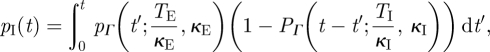
To fully explain the difference in the levels of persistence of the models in Keeling & Grenfell (2002), we need to consider the interaction of seasonality in transmission and the WTD on a shorter time scale. On a scale of the order of the infectious period, we might expect considerable variation in an individual's R₀ when the transmission parameter changes significantly. Individuals infected around the break-up and commencement of school terms will lead to a different number of secondary cases for different WTDs. We can construct the expected response of the reproductive ratio for different WTDs by convolving the probability of being infectious (as a function, p_I(t), of time since infection) with the term-time forcing function.

We define the individual basic reproductive ratio as a convolution

3.2

Because β(t) has period equal to the school year, R_indiv(t) is also therefore defined to be a periodic function. We calculate the value of R_indiv for each day of the year numerically using the values of β_t and the convolution theorem for Fourier transforms (Riley et al. 2002). This definition makes the assumption that the transmission parameter is constant across individuals and the variation in the reproductive number is purely due to the WTD and the form of the seasonal forcing function β(t). This is therefore a special case of the instantaneous reproductive number (Fraser 2007) of Kermack–McKendrick type time-since-infection models (Kermack & McKendrick 1927). Essentially, R_indiv is the basic reproductive ratio of the pathogen, R₀, for individuals who become infected on a specific day—a running average of the underlying binary step structure of β with a kernel given by the WTD.

We can derive an expression for p_I(t) by assuming that the latent and infectious periods are gamma-distributed with shape parameters κ_I, κ_E and scale parameters θ_I, θ_E. The probability density function for the time an individual is infectious is then

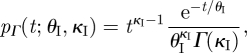3.3

where Γ(κ_I) is the gamma function . We can control the dispersion of the WTD using the shape parameter κ_I (coefficient of variation of gamma ), adjusting θ_I to maintain a constant mean value (T_I = κ_Iθ_I). For integral values of the shape parameter, the gamma distribution (equation (3.3)) arises from a sum of independent, identical, exponential terms. This property allows gamma distributions to be straightforwardly incorporated within standard compartmental models by subdividing the infectious and latent classes into stages (the number of which are identical to the shape parameter of the gamma distribution).

The probability of being infectious at time t after entering the infectious state is

3.4

where P_Γ is the cumulative distribution function and θ_I is the reciprocal of the infectious period (T_I = 5 days). Accounting for the latent period distribution (of mean duration T_E = 8 days) using the law of total probability gives the required expression

3.5

where κ_E is the shape parameter for the latent period distribution.

The magnitude of the drop in R_indiv in response to the fall in transmission during a vacation period (β(t) = β_L) is dependent on the length of the vacation and inversely related to the dispersion of the WTDs, i.e. as κ_E, κ_I increase, the temporal variation in R_indiv decreases (figure 3a). The sinusoidal forcing function generates a pattern which is in sharp contrast to term-time forcing, with much less marked variation in R_indiv owing to the smoother underlying pattern in transmission (figure 3b). We would therefore expect that WTDs will have most impact on model fitting when there exist sharp discontinuities, such as term-time effects, in the underlying transmission process.

Figure 3.

Interaction between seasonal forcing and the WTD. (a) The individual reproductive ratio for a term-time forcing function (R₀ = 17.0, α = 0.17) resulting from gamma-distributed WTDs in the latent and infectious stages with shape parameters κ_E = κ_I = κ. Dates of school terms are quoted in the electronic supplementary material. Black line, κ = 1; blue line, κ = 2; red line, κ = 5; green line, κ = 20. (b) The individual reproductive ratio for a cosine forcing function (R₀ = 17.0, α = 0.17) resulting from gamma-distributed WTDs in the latent and infectious stages with shape parameters κ_E = κ_I = κ. (c) Detail on the response of the individual reproductive ratio to the autumn half-term holiday. Parameters as in (a). (d) The individual reproductive ratio calculated for the trajectory-matched model fits from Keeling & Grenfell (2002). Transmission rates are reproduced in the electronic supplementary material (table a). Black lines are the two models with exponential WTDs (κ_E = κ_I = 1), red lines the two gamma (8,5) models (with κ_E = 8, κ_I = 5).

Comparing R_indiv for the range of previously published ‘best-fit’ models for London, we find that the trajectory-matching method is equivalent to fitting the response of R_indiv for the first (which happens to be the shortest) vacation of the year—the autumn half-term holiday—with all model fits corresponding closely at this point (figure 3d). Given that the autumn half-term holiday occurs during the attack of the major epidemic—and the impact of it is particularly sensitive to the WTD (figure 3c)—it is natural that it is this response that is picked out by trajectory-matching methods. The requirement that models correspond in their response to the autumn half-term holiday implies that models with less dispersed infectious period distributions will always have a lower amplitude of seasonal variation in R_indiv and therefore a higher R_indiv in the long summer holiday (days 313–365, counting from the beginning of the school year) where the majority of extinction events occur.

4. Persistence of the simple model

In this section, we review the persistence properties of homogeneous mixing SEIR models of measles with exponential and gamma-distributed infectious (and latent) periods under the criteria of constant parameters and trajectory-matched dynamics. Persistence characteristics of models are obtained by the numerical simulation of a fully stochastic, seasonally forced, SEIR model which we refer to as the simple model (see technical appendix for details).

We have argued that parametric differences are introduced when models with different WTDs are required to match the same major epidemic dynamics in a historical time series. We now revisit the persistence characteristics of trajectory-matched models and compare the qualitative patterns of persistence under the alternative criterion of maintaining constant parameters. For the purposes of this comparison, we use a rate of imports of infection which is scaled with the square root of population size (0.02 per year; Keeling & Grenfell 2002).

We take advantage of the increase in the available computational power to generate a larger number of ensemble replicate simulations than in the previous studies. One hundred replicates of 24 years (approx. equal to the longest pre-vaccination time series of measles reports available for England and Wales) were generated for each population size and model parametrization. We quantify persistence using the three measures introduced in §2: MAFs, FPE and FPI.

4.1. Constant parameters versus trajectory-matched dynamics

In figure 4a,b, we compare the persistence of models with different WTDs using the ensemble average (over 100 replicates of 24 years) of MAFs. The WTDs in the latent and infectious classes are modelled once more as gamma distributions, using the method of stages (Anderson & Watson 1980). The infectious and latent classes are subdivided into κ_E and κ_I compartments with a constant rate of flow between the compartments set at κ_E/T_E and κ_I/T_I to maintain the mean time spent in the latent (T_E = 8 days) and infectious (T_I = 5 days) classes. κ_E and κ_I are therefore limited to take integral values. The exponential model corresponds to the limiting case of κ_E = 1 and κ_I = 1, with increasing values of κ_E and κ_I reducing the dispersion of the WTDs. Modifying the WTDs leads to a correction to the algebraic form of R₀ which is small, of the order of mortality rate (μ) (Lloyd 2001b). For all of the model simulations presented here, stages of 1 day were used for the gamma model (κ_E = 8, κ_I = 5), henceforth the gamma (8,5) model, to maintain consistency with Keeling & Grenfell (2002).

Under the constant parameter comparison, both the exponential and the gamma (8,5) models have fixed R₀ = 17.0, α = 0.17. For the trajectory-matched comparison, we consider a pair of trajectory-matched models with (R₀ = 17.522, α = 0.2535) for the exponential model and (R₀ = 17.2991, α = 0.1984) for the gamma (8,5) model.

We find that, when scaling the level of infective imports with population size, all models predict a similar level of the CCS lying between 500 000 and 1 million, albeit predicting greater levels of persistence overall in smaller populations than the data would suggest. Under both criteria (constant parameters versus trajectory-matched dynamics), the gamma (8,5) model appears to exhibit greater persistence in populations smaller than the CCS, in line with the predictions of Keeling & Grenfell (1998). However, under the constant parameters comparison, the fade-out curves cross over (close to the CCS) with the exponential model exhibiting marginally greater persistence in the large population limit (populations larger than the CCS).

4.2. Sensitivity to measure of persistence

We have already discussed the potentially misleading properties of the mean number of annual fade-outs as a measure of persistence (§2; quantifying persistence, figure 1) and argued that the proportion of FPE could provide a more consistent description of epidemic persistence. Calculating the ensemble average of FPE from the same model simulations, we find that the relative patterns of persistence between the exponential and the gamma (8,5) models are dramatically different from those suggested by MAFs. In terms of the FPE, the exponential model exhibits greater persistence than the gamma (8,5) model over the whole range of population sizes considered for both the trajectory-matched and the constant parameter models.

The seemingly opposite conclusions suggested by these two persistence measures can be resolved by repeating the comparison once again using our final persistence measure—FPI. With a threshold value of T = 1 (chosen such that the FPIs are calculated from the same subset of epidemics as the MAFs), the FPI for the exponential and gamma (8,5) models displays the same relative patterns of persistence (figure 5a,b) suggested by the MAFs (figure 4a,b). Under this persistence measure, there is once again a clear crossing over of the fade-out curves—with the gamma model exhibiting greater persistence in small populations. However, when the value of T is increased to T = 5 (figure 5c,d; excluding all of the small invasive outbreaks where the number of weekly reports of measles never exceeds 5), the exponential model exhibits greater persistence over the entire range of population sizes in line with the comparison under FPE.

It should finally be noted that the differences in persistence between all of the models, no matter the choice of persistence measures, only become apparent when comparing the ensemble average over multiple replicate simulations. In particular, in the range of population sizes relating to the estimated level of the CCS (250 000–500 000), all of the models exhibit similar levels of persistence. This agreement with the data is guaranteed by the choice of a rate of infectious imports which leads to levels of persistence comparable with the data. The dynamics of forced SEIR models are known to be exceedingly sensitive to differing rates of infective imports (Engbert & Drepper 1994; Bolker & Grenfell 1995). The quantitative differences in persistence between models can be modified somewhat by the rate of imports (results not shown). The differences between models are still small compared to the impact of varying the import rate itself.

5. RAS Models

Serological surveys (Anderson & May 1982, 1983, 1985; Edmunds et al. 2000) and the analysis of age-structured cases reports (Wilson 1904; Collins 1924, 1929; Sydenstricker 1928; Godfrey 1930; Hedrich 1930) reveal that the probability of acquiring measles varies substantially with age. In industrial countries before vaccination, there is a generally consistent pattern of a peak in transmission for 5 to 10-year-old children. Incidence data show a clear link between the epidemic timing and the pattern of school terms (Fine & Clarkson 1982). This implies that the heterogeneity in mixing with age is the consequence of higher mixing rates of school-age children within the classroom (Schenzle 1984).

The availability of parallel age-structured prevalence data and weekly incidence data has allowed detailed, dynamic, age-structured models to be developed for England and Wales (Schenzle 1984). These so-called RAS models have notably been used in the modelling of persistence (Bolker & Grenfell 1993) and forecasting the impact of vaccination (Babad et al. 1994). RAS models explicitly account for the age dependence of transmission and are therefore a more biologically realistic description of measles epidemiology than models assuming homogeneous mixing.

The PRAS model (Keeling & Grenfell 1997) demonstrated an order of magnitude smaller CCS than the previously published RAS models. This result was attributed to the use of less dispersed WTDs, a mechanism which the simulations presented in the previous section bring into doubt. The PRAS model introduced several innovations which modified the parametrization of the model somewhat from the previous RAS models, the most significant of which was using an approximate fractional ageing method (discussed below).

We compare the persistence characteristics of the PRAS model with two earlier RAS models which we refer to as the Bolker model (Bolker & Grenfell 1993) and the Babad model (Babad et al. 1994). We take the same approach as with the simple model, quantifying the differences in parametrization before comparing persistence characteristics by numerical simulation.

5.1. RAS model framework

The proper accounting of age structure within an epidemic model necessitates a considerable increase in model complexity over the simple model. Theoretically, transmission parameters and the proportions of the population SEIR will vary continuously with age. A formulation based on partial differential equations would be the most natural formulation (Anderson & May 1991). Such systems are notoriously difficult to simulate efficiently—particularly with the incorporation of stochasticity. At best, the data can provide us with differences in transmission between birth cohorts or broad age classes. We can therefore considerably simplify our model by considering only coarse yearly cohorts, and assume that transmission parameters only vary between broad age classes determined by the grain of the data (Schenzle 1984; Anderson & May 1991). In addition to the computational advantages, this approach is arguably more epidemiologically correct as it is a child's (school) year group which determines their disease risk rather than their calendar age.

Each compartment of the simple model (S,E,I,R) is further subdivided into discrete age classes with bounds a₁, a₂, a₃, … , a_n and of widths Δa₁, Δa₂, Δa₃, … , Δa_n. Serological studies reveal that newborns are protected from measles through maternally transferred antibodies, for a period that typically ranges between three and six months (Cáceres et al. 2000). In industrial countries, such as England and Wales, this period is of little epidemiological importance and exceedingly short compared to the mean age of infection. For completeness this is accounted for in the RAS framework by the inclusion of a fifth epidemiological compartment, M, for maternally protected infants who are transiently immune to infection.

The frequency-dependent formulation of the force of infection used in the simple model must be generalized to take into account different transmission parameters between age classes

5.1

The transmission parameter assumed for homogeneous mixing is replaced with a matrix, β. This matrix defines the coupling between susceptibles in age class i with infectives in age class j. The instantaneous force of infection acting on an age class is a sum of the total infectives in the population by age, weighted by the elements of β. Assuming that the population is in demographic equilibrium and fully susceptible, a basic reproductive ratio can be defined for the expected number of new infections within a given age group when a single infectious individual is introduced into a second age group. Together, these age-group specific basic reproductive ratios form the next generation matrix K (Diekmann et al. 1990), which has elements

5.2

where T_I is the average length of the infectious period and w_i is the proportion of the population that is contained within the ith age class. Under the assumption of a type I survival function (Anderson & May 1991) w_i = Δa_i/L, where L is the life expectancy in the population.

We can interpret β_ijw_i as the potential number of effective contacts per unit time between an infectious individual in age class j with susceptible individuals in age class i (Wallinga et al. 2001). Therefore, each element of K gives the expected number of secondary cases within age class i on introduction of a single infective into age class j. The basic reproductive ratio, R₀, is given by the dominant eigenvalue of K. In the same way that the effective reproductive ratio R is reduced by the buildup of immunity in a population, an age profile of susceptibility σ_i (defined as the proportion of age class i which is susceptible) leads to a reduction in the observed reproductive ratios

5.3

The overall effective reproductive ratio (R) in an age-stuctured population will therefore be given by the dominant eigenvalue of R_ij.

5.1.1. The WAIFW matrix

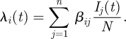
The structure of β, often referred to as the ‘who acquires infection from whom’ (WAIFW) matrix (Anderson & May 1991), determines the dynamics of the model and the long-term age distribution of susceptibility. Yet, as with the mean transmission parameter of the simple model, we cannot directly measure the values of this matrix directly from data. Although some novel methods for estimating mixing rates empirically have been suggested (Edmunds 1997; Mossong et al. 2007), in general the only constraint on the elements of β is that they reproduce the long-term average force of infection λ_i, or equivalently the serological age profile of susceptibility σ_i. There is therefore considerable scope for a whole spectrum of WAIFW matrices (with widely varying transmission parameters and basic reproductive ratios) to fit the same force of infection data. Models for England and Wales typically concentrate transmission in the core group of 5 to 10-year-olds in line with the peak in transmission in school-age children (Anderson & May 1991) and term-time forcing hypothesis.

RAS models with different values of R₀ can match the same levels of incidence in an endemic population provided that they generate the same age profile of incidence and share a similar overall effective reproductive ratio R. All of the models considered here have different values of R₀ (PRAS 10.6, Babad 8.6, Bolker 5.5) but share a similar effective reproductive ratio R at a fixed birth rate of 13.3 per 1000. (Details of the parametrization of these models can be found in the technical appendix, §2.)

5.2. Impact of fractional ageing on parametrization of RAS models

In the original RAS model, annual age classes were used (Schenzle 1984). Birth is a continuous process into the first age class, which is emptied into the next age class annually. Successive cohorts are promoted to higher age classes annually, so we refer to this as a cohort ageing method. This discrete ageing method leads to an additional source of seasonal forcing in RAS models (beyond the term-time forcing which is also included in homogeneous mixing models) resulting from the injection of susceptible children starting school for the first time.

Keeling & Grenfell (1997) introduced a fractional ageing method, where the numbers of individuals in each epidemiological state are classified only within the five coarse age groups (a_i with age ranges 0–5, 5–10, 10–15, 15–25, 25+) relating to the structure of the epidemiological data. Rather than ageing a whole birth cohort, each year a constant fraction 1/Δa_i is aged.

This assumption introduces considerable computational advantages, reducing the number of compartments in the model to the minimum required detail to model the available data. However, the implication of this assumption is that the proportion of susceptibles moving between mixing classes is altered. Keeling & Grenfell (1997) assumed that the dynamical consequence of this approximation would be accounted for by their trajectory-matching methodology. We can calculate the static age distribution which we would expect in models with cohort and fractional ageing by calculating the flux of susceptible individuals moving between the coarse age groups (see technical appendix). We see (figure 6) that the fractional ageing method leads to a higher proportion of susceptibles in the peak transmission (5–10 year) age class as compared to cohort ageing.

Figure 6.

Static age distributions under cohort and fractional ageing. The predicted susceptible proportion, before and after ageing, in infants (0–5), primary school children (5–10), adolescents (10–20) and adults (20+) under (a) fractional ageing and (b) cohort ageing. Proportions are calculated based on the form of the force of infection assumed by the PRAS model. Details of this calculation can be found in the electronic supplementary material (§3). Blue rectangle, start of year; red rectangle, end of year.

This modification to the age profile of susceptibility is liable to modify the effective reproductive ratio R for the PRAS model as compared to a model using an accurate ageing method. Given the importance of the core group in driving the dynamics of RAS models, the increased flux of susceptibles that a coarse age grain affords should give a significant advantage for persistence in the minor epidemic year. Seasonality in transmission and incidence will substantially alter the predicted age profile from this static analysis. In order to test this hypothesis, we must resort again to using numerical simulation, comparing cohort ageing, and coarse age-grained models, with different WTDs.

5.3. Persistence in RAS models

For consistency with previously published studies (Bolker & Grenfell 1995; Keeling & Grenfell 1997), we compare the persistence properties of RAS model under the assumption of a rate of infective imports which is not scaled by population size and fixed at 10 imports per year. It should be noted that, although not previously reported, Keeling & Grenfell (1997) shaped this import rate by the average deterministic biennial attractor of the PRAS model. This approximation was intended to mimic the seasonal fluctuations in import rates likely to occur in real populations. Introducing this extra layer of complexity does not qualitatively change the results of this section, so we take the simpler assumption here of a fixed (non-seasonal) rate of imports (see technical appendix for more details).

In figure 7, we revisit the comparison from Keeling & Grenfell (1997) using the newly introduced persistence measures of FPE and FPI. We compare the persistence of a suite of RAS models with different parametrizations (differing by their WAIFW matrices and amplitude of term-time forcing) using fractional and cohort ageing methods (figure 7).

Figure 7.

Persistence in age-structured models: fractional versus cohort ageing. PRAS, Bolker and Babad models use transmission parameters estimated by Keeling & Grenfell (1997), Bolker & Grenfell (1995) and Babad et al. (1994), respectively. The shape parameters used for the (gamma distributed) infectious and latent periods for each model are indicated by parentheses (κ_E, κ_I). (a,b) Ensemble average (over 100 replicates of 24 years) of fade-outs post epidemic against population size for (a) fractional and (b) cohort ageing (T = 1/2000 per capita). (c,d) Ensemble average (over 100 replicates of 24 years) of fade-outs post invasion against population size for (c) fractional and (d) cohort ageing (T = 1). Shaded envelope represents a 95 per cent confidence interval calculated as 1.96 standard errors, based on 100 replicates of 24 years. Imports of infection are fixed (independent of population size) at 10 infectious imports per year. Black line, PRAS (1,1); red line, PRAS (8,5); blue line, Bolker (1,1); green line, Babad (1,1).

We first note that the fractional ageing models (figure 7a,c) all demonstrate markedly greater persistence than the more accurate cohort based models (figure 7b,d). We present three different model parametrizations for comparison under the fractional ageing method: PRAS (1,1), PRAS (8,5), Bolker (1,1). PRAS (8,5), red lines, is the original PRAS model published by Keeling & Grenfell (1997; i.e. a gamma (8,5) model with PRAS transmission parameters and fractional ageing). We re-fitted this model to produce the same qualitative dynamics in a model with exponential WTDs (PRAS (1,1), black lines), using a trajectory-matching technique (Conlan 2006). Under this comparison, we see similar relative patterns of persistence between the PRAS (1,1) and the PRAS (8,5) models as those presented earlier (§4) for the homogeneous mixing model (figures 4 and 5).

The order of magnitude difference between exponential and gamma (8,5) models reported by Keeling & Grenfell (1997) is not apparent between these two appropriately parametrized models (figure 7a,c). The comparison made in Keeling & Grenfell (1997) was made with a fractional ageing model using the Bolker transmission parameters (Bolker (1,1), blue lines) unadjusted for the novel fractional ageing method (figure 7a,c). The dramatic difference in persistence is therefore attributable not to the WTD, but to the differences in the transmission parameters between the Bolker and the PRAS WAIFW matrices.

In the final comparison, we compare the persistence characteristics of RAS models with three different transmission matrices (PRAS, Bolker and Babad) and exponential WTDs under the more accurate cohort ageing model (figure 7b,d). Once again, the PRAS transmission matrix is corrected by a small reduction in the core-group transmission parameter in order to achieve the fairest comparison (i.e. maintaining the same trajectory-matched dynamics). With an accurate ageing model, the persistence of the PRAS model falls in line with the previously published Bolker and Babad models. We conclude that the increase in persistence reported by Keeling & Grenfell (1997) was a consequence of the approximate ageing model.

6. Discussion

We have addressed the controversy over the effect of more realistic, less dispersed, WTDs on the persistence of measles. Using numerical simulations, we illustrate that—depending on the measure of persistence which is used—the introduction of realistic WTDs can both increase (Keeling & Grenfell 2002) and decrease (Lloyd 2001c) the persistence of measles, as compared to the exponential model (figures 4 and 5).

The ‘Keeling and Grenfell’ effect—of enhanced persistence for models with gamma-distributed WTDs—appears to be limited to the small outbreaks between major epidemics which are generated in models with a small rate of infective imports. We have shown that when these small ‘invasion’ epidemics are removed from the calculation of the persistence measure (essentially by changing our definition of what constitutes an epidemic), the exponential model exhibits greater persistence across the range of population sizes and ‘realistic’ parameter regimes considered in this paper (figure 5). This observation helps to unify the apparently contradictory results of Lloyd (2001c) and Keeling & Grenfell (2002).

The fundamental difference between these two studies ultimately lies in the authors' differing interpretation of what persistence means. The CCS as a philosophical concept relates to isolated populations. However, in isolation any stochastic population model will eventually become extinct. Any measure of persistence is therefore implicitly tied to a time scale of observation. In his theoretical studies, Lloyd assessed the persistence of disease by calculating the proportion of simulations which faded out in a truly isolated population over a period of 10 years (Lloyd 2001c). Philosophically, this comparison is more resonant with the notion of the CCS as an isolated community concept and most closely corresponds to the probability of fade-out occurring after a large epidemic.

Keeling and Grenfell's approach, comparing the frequency of fade-outs under a rate of imports of infection, additionally captures the persistence between large epidemics. The time scale of observation of persistence is therefore dependent on the rate of infectious imports and the definition of the fade-out statistic. This comparison inevitably measures both the persistence after an epidemic and the persistence during small invasion epidemics. The MAFs can lead to a misleading comparison between different models leading to greater relative enhancement of persistence (figure 4) than is evident under other persistence measures (figures 4 and 5). However, we find that, no matter the measure of persistence, models fitted to the historical patterns of incidence in England and Wales (specifically London) predict a CCS within a realistic range regardless of the choice of WTD (figures 4 and 5).

Lloyd chose to investigate the impact of different WTDs by comparing models with identical parameters (Lloyd 2001c), specifically fixing R₀ and the amplitudes of seasonal forcing. Given the independent estimates of these quantities, this would indeed be the stronger comparison as we could select between models on the basis of which provides a closer representation of the historical data. Despite recent advances in the estimation of sociological contact patterns (Brockmann et al. 2006; Mossong et al. 2007), in practice transmission parameters must, in some way, be inferred from epidemic time-series data and serological profiles of susceptibility.

In the large population limit, models of infectious diseases must, at a minimum, be able to match the historical patterns of incidence. Estimates of transmission parameters are known to be sensitive to the assumptions of the WTD (Lloyd 2001a; Wearing et al. 2005; Heffernan & Wahl 2006; Wallinga & Lipsitch 2007). This necessitates that the parametrization of models whose parameters are obtained by trajectory matching must change with different WTDs. We use a simple construction, the individual reproductive ratio R_indiv, to demonstrate the subtleties of the interaction of the WTD with term-time forcing functions. The distribution of waiting times in the exposed and infectious states attenuates our ability to estimate the amplitude of seasonality in transmission parameters. We would expect this attentuation to affect the structure of any statistical estimates of the instantaneous reproductive ratio (R) from time series (Finkenstadt & Grenfell 2000; Fraser 2007; Cauchemez & Ferguson 2008). At the very least, the dispersion of WTDs will affect the fidelity with which we can estimate the seasonal patterns in transmission.

Keeling & Grenfell (2002) compared models with different WTDs which were fitted to the historical time series of measles incidence for London before vaccination. We argue that the fitting method introduced systematic parametric differences between models with different WTDs, notably in the basic reproductive ratio R₀. However, these differences do not affect the qualitative comparison between the persistence of the exponential and gamma-distributed models which is identical under Lloyd's comparison criteria of equal parameters (Lloyd 2001c).

The dramatic reduction of the level of the CCS reported for the PRAS model (Keeling & Grenfell 1997) cannot be attributed to the use of less dispersed WTDs. The fractional ageing assumed by the PRAS model may provide an excellent match to the dynamics of England and Wales; however, it is not a true representation of the age structure of a real population. Restoration of an accurate, cohort-based, ageing model leads to levels of persistence consistent with previously published studies (Bolker & Grenfell 1995). The qualitative comparison between the exponential and the gamma-distributed models was exaggerated by the use of different transmission matrices for the RAS and PRAS models—with a theoretical R₀ for the PRAS model twice as large as the RAS model.

Simple epidemic models of measles can account for both the dynamics and the persistence of measles in England and Wales provided there is a rate of infective imports which is scaled by the population size (Keeling & Rohani 2007). However, we should be cautious about interpreting what this means for the CCS of measles in a truly isolated population. Given a large enough rate of infectious imports, we can all but guarantee the persistence of measles in a population of any size. On the other hand, it would be just as unreasonable to expect theoretical models of transmission for England and Wales to exhibit the correct levels of persistence without some accounting for the re-introduction of disease after fade-out (Grenfell et al. 2001).

Age structure and the detailed distribution of the infectious and latent period distributions can modify the overall patterns of persistence. With the inclusion of infective imports which scale with the population size, explicitly age-structured models will also predict similar levels for the CCS (Conlan 2006). For some measures of persistence, the Babad and Bolker models demonstrate different levels of persistence (figure 7d) in line with their respective values of R₀ (8.6 versus 5.5). Current RAS models assume a particular form of WAIFW matrix, which effectively sets the value of R₀ and limits the way in which seasonality in transmission can be modelled while remaining consistent with the historical data (technical appendix 3.4.5). Consequently, seasonality in transmission has been treated in a very ad hoc and inconsistent fashion between different RAS models. Novel research on the structure of mixing patterns in populations (Mossong et al. 2007) and specifically within schools (Eames & Conlan 2008) may allow us to select between WAIFW matrices on a more quantitative basis. In turn, this should allow for the development of more refined age-structure models from which seasonality can be estimated in a more rigorous fashion.

We must conclude that the assumptions concerning spatial imports of infection are the primary determinant of persistence in theoretical, single population, models. In reality, and in spatial network models, there will be considerable feedback between the rates of extinction in subpopulations and the effective rates of epidemiological coupling. Although our results cannot be directly related to explicitly spatial epidemic models, they suggest that the differences between models with different latent and infectious period distributions (in terms of persistence and epidemic thresholds) will be most pronounced in weakly coupled networks of small host populations, in contrast to the core-satellite dynamics exhibited by childhood diseases in England and Wales (Grenfell et al. 2001). A definitive understanding of the processes necessary for explaining the level of the CCS for measles must incorporate spatial processes explicitly. The persistence and spatial dynamics of measles cannot be separated from each other.

References

- Anderson D., Watson R. 1980. On the spread of a disease with gamma distributed latent and infectious periods. Biometrika 67, 191–198. ( 10.1093/biomet/67.1.191) [DOI] [Google Scholar]
- Anderson R. M., May R. M. 1982. Directly transmitted infectious diseases: control by vaccination. Science 215, 1053–1060. ( 10.1126/science.7063839) [DOI] [PubMed] [Google Scholar]
- Anderson R. M., May R. M. 1983. Vaccination against rubella and measles: quantitative investigations of different policies. J. Hyg. Camb. 94, 365–436. [DOI] [PMC free article] [PubMed] [Google Scholar]
- Anderson R. M., May R. M. 1985. Age related changes in the rate of disease transmission: implications for the design of vaccination programmes. J. Hyg. Camb. 94, 365–436. [DOI] [PMC free article] [PubMed] [Google Scholar]
- Anderson R. M., May R. M. 1991. Infectious diseases of humans: dynamics and control. New York, NY: Oxford University Press. [Google Scholar]
- Andersson H., Britton T. 2000. Stochastic epidemics in dynamic populations: quasi-stationarity and extinction. J. Math. Biol. 41, 559–580. ( 10.1007/s002850000060) [DOI] [PubMed] [Google Scholar]
- Babad H. R., Nokes D. J., Gay N. J., Miller E., Morgan-Capner P., Anderson R. M. 1994. Predicting the impact of measles vaccination in England and Wales: model validation and analysis of policy options. Epidemiol. Infect. 114, 319–344. ( 10.1017/S0950268800057976) [DOI] [PMC free article] [PubMed] [Google Scholar]
- Bailey N. 1954. A statistical method for estimating the periods of incubation and infection of an infectious disease. Nature 174, 139–140. ( 10.1038/174139a0) [DOI] [PubMed] [Google Scholar]
- Bailey N. 1964. Some stochastic models for small epidemics in large populations. Appl. Stat. 13, 9–19. ( 10.2307/2985218) [DOI] [Google Scholar]
- Bailey N. 1975. The mathematical theory of epidemics. London, UK: Griffin. [Google Scholar]
- Bartlett M. 1956. Deterministic and stochastic models for recurrent epidemics. Proc. 3rd Berkeley Symp. on Mathematical Statistics and Probability, vol. 4 (ed. Neyman J.), pp. 81–109. Berkeley, CA: University of California Press. [Google Scholar]
- Bartlett M. 1957. Measles periodicity and community size. J. R. Stat. Soc. A 120, 48–70. ( 10.2307/2342553) [DOI] [Google Scholar]
- Bauch C. T., Earn D. J. D. 2003. Transients and attractors in epidemics. Proc. R. Soc. Lond. B 270, 1573–1578. ( 10.1098/rspb.2003.2410) [DOI] [PMC free article] [PubMed] [Google Scholar]
- Begon M., Bennett M., Bowers R., French N., Hazel S., Turner J. 2002. A clarification of transmission terms in host-microparasite models: numbers, densities and areas. Epidemiol. Infect. 129, 147–153. ( 10.1017/S0950268802007148) [DOI] [PMC free article] [PubMed] [Google Scholar]
- Bjornstad O. N., Finkenstadt B., Grenfell B. T. 2002. Dynamics of measles epidemics. I. Estimating scaling of transmission rates using a time series SIR model. Ecol. Monogr. 72, 169–184. [Google Scholar]
- Black F. L. 1966. Measles endemicity in insular populations: critical community size and its evolutionary implication. J. Theor. Biol. 11, 207–211. ( 10.1016/0022-5193(66)90161-5) [DOI] [PubMed] [Google Scholar]
- Black F. L. 1984. Measles In Viral infections of humans—epidemiology and control (ed. Evans A.), ch. 15, 2nd edn. New York, NY: Plenum Medical Book Co. [Google Scholar]
- Blythe S., Anderson R. 1988. Distributed incubation and infectious periods in models of the transmission dynamics of the human immunodeficiency virus (HIV). IMA J. Math. Appl. Med. Biol. 5, 1–19. ( 10.1093/imammb/5.1.1) [DOI] [PubMed] [Google Scholar]
- Bolker B. M., Grenfell B. T. 1993. Chaos and biological complexity in measles epidemics. Proc. R. Soc. Lond. B 251, 75–81. ( 10.1098/rspb.1993.0011) [DOI] [PubMed] [Google Scholar]
- Bolker B. M., Grenfell B. T. 1995. Space, persistence and dynamics of measles epidemics. Phil. Trans. R. Soc. Lond. B 348, 309–320. ( 10.1098/rstb.1995.0070) [DOI] [PubMed] [Google Scholar]
- Brockmann D., Hufnagel L., Geisel T. 2006. The scaling laws of human travel. Nature 439, 462–465. ( 10.1038/nature04292) [DOI] [PubMed] [Google Scholar]
- Broutin H., Mantilla-Beniers N., Simondon F., Aaby P., Grenfell B. T., Gueǵan J. F., Rohani P. 2005. Epidemiological impact of vaccination on the dynamics of two childhood diseases in rural Senegal. Microbes Infect. 7, 593–599. [DOI] [PubMed] [Google Scholar]
- Cáceres V. M., Strebel P. M., Sutter R. W. 2000. Factors determining prevalence of maternal antibody to measles virus throughout infancy: a review. Clin. Infect. Dis. 31, 110–119. ( 10.1086/313926) [DOI] [PubMed] [Google Scholar]
- Cauchemez S., Ferguson N. M. 2008. Likelihood-based estimation of continuous-time epidemic models from time-series data: application to measles transmission in London. J. R. Soc. Interface 5, 885–897. ( 10.1098/rsif.2007.1292) [DOI] [PMC free article] [PubMed] [Google Scholar]
- Collins S. 1924. Past incidence of certain communicable diseases common among children. Public Health Rep. 36, 1553–1567. [Google Scholar]
- Collins S. 1929. Age incidence of the common communicable diseases of children. Public Health Rep. 44, 763–829.19315185 [Google Scholar]
- Conlan A. J. K. 2006. Modelling measles epidemics in high birth rate countries. PhD thesis, University of Cambridge, UK. [Google Scholar]
- Conlan A. J. K., Grenfell B. T. 2007. Seasonality and the persistence and invasion of measles. Proc. R. Soc. B 274, 1133–1141. ( 10.1098/rspb.2006.0030) [DOI] [PMC free article] [PubMed] [Google Scholar]
- Diekmann O., Heesterbeek J., Metz J. 1990. On the definition and the computation of the basic reproduction ratio R0 in models for infectious diseases in heterogenous populations. J. Math. Biol. 28, 365–382. ( 10.1007/BF00178324) [DOI] [PubMed] [Google Scholar]
- Dietz K. 1976. The incidence of infectious diseases under the influence of seasonal fluctuations. In Lecture notes in biomathematics, vol. 11, pp. 1–15. Berlin, Germany: Springer. [Google Scholar]
- Eames K. T. D., Conlan A. J. K. 2008. Mixing patterns in primary schools: classrooms, playgrounds and transmission. In Transmission Conf., University of Warwick, UK. [Google Scholar]
- Earn D. J. D., Rohani P., Grenfell B. T. 1998. Persistence, chaos and synchrony in ecology and epidemiology. Proc. R. Soc. Lond. B 265, 7–10. ( 10.1098/rspb.1998.0256) [DOI] [PMC free article] [PubMed] [Google Scholar]
- Earn D. J. D., Rohani P., Bolker B. M., Grenfell B. T. 2000. A simple model for complex dynamical transitions in epidemics. Science 287, 667–670. ( 10.1126/science.287.5453.667) [DOI] [PubMed] [Google Scholar]
- Edmunds W. 1997. Who mixes with whom? A method to determine the contact patterns of adults that may lead to the spread of airborne infections. Proc. R. Soc. Lond. B 264, 949–957. ( 10.1098/rspb.1997.0131) [DOI] [PMC free article] [PubMed] [Google Scholar]
- Edmunds W. J., Gay N. J., Kretzschmar M., Pebody R. G., Wachmann H. 2000. The pre-vaccination epidemiology of measles, mumps and rubella in Europe: implications for modelling studies. Epidemiol. Infect. 125, 635–650. ( 10.1017/S0950268800004672) [DOI] [PMC free article] [PubMed] [Google Scholar]
- Engbert R., Drepper F. 1994. Qualitative analysis of unpredictability: a case study from childhood epidemics. In Predictability and nonlinear modelling in natural sciences and economics, pp. 204–215. Dordrecht, The Netherlands: Kluwer. [Google Scholar]
- Ferrari M., Grais R., Bharti N., Conlan A., Bjornstad O., Wolfson L., Guerin P., Djibo A., Grenfell B. 2008. The dynamics of measles in sub-Saharan Africa. Nature 451, 679–684. ( 10.1038/nature06509) [DOI] [PubMed] [Google Scholar]
- Fine P. E. M., Clarkson J. A. 1982. Measles in Engand and Wales—I: an analysis of factors underlying seasonal patterns. Int. J. Epidemiol. 11, 5–14. ( 10.1093/ije/11.1.5) [DOI] [PubMed] [Google Scholar]
- Finkenstadt B. F., Grenfell B. T. 2000. Time series modelling of childhood diseases: a dynamical systems approach. J. R. Stat. Soc. C 49, 187–205. [Google Scholar]
- Fraser C. 2007. Estimating individual and household reproduction numbers in an emerging epidemic. PLoS One 2, pe758. ( 10.1371/journal.pone.0000758) [DOI] [PMC free article] [PubMed] [Google Scholar]
- Godfrey E. 1930. The age distribution of communicable diseases according to size of community. Public Health 18, 616–631. [DOI] [PMC free article] [PubMed] [Google Scholar]
- Goodman D. 1987. The demography of chance extinction. Viable populations for conservation (ed. Soulé M.). Cambridge, UK: Cambridge University Press. [Google Scholar]
- Grenfell B. T., Bjornstad O. N., Kappey J. 2001. Travelling waves and spatial hierarchies in measles epidemics. Nature 414, 716–723. ( 10.1038/414716a) [DOI] [PubMed] [Google Scholar]
- Grenfell B. T., Bjornstad O. N., Finkenstadt B. 2002. Dynamics of measles epidemics. II. Scaling noise, determinism and predictability with the time series SIR model. Ecol. Monogr. 72, 169–184. [Google Scholar]
- Grossman Z. 1980. Oscillatory phenomena in a model of infectious diseases. Theor. Popul. Biol. 18, 204–243. ( 10.1016/0040-5809(80)90050-7) [DOI] [PubMed] [Google Scholar]
- Hanski I. A., Gaggiotti O. E. 2004. Ecology, genetics and evolution of metapopulations. London, UK: Academic Press. [Google Scholar]
- Heffernan J., Wahl L. 2006. Improving estimates of the basic reproductive ratio: using both the mean and the dispersal of transition times. Theor. Popul. Biol. 70, 135–145. ( 10.1016/j.tpb.2006.03.003) [DOI] [PMC free article] [PubMed] [Google Scholar]
- Hedrich A. 1930. The corrected average attack rate from measles among city children. Am. J. Hyg. 11, 576–600. [Google Scholar]
- He D., Ionides E. L., King A. A. In press Plug-and-play inference for disease dynamics: measles in large and small populations as a case study. J. R. Soc. Interface. ( 10.1098/rsif.2009.0151) [DOI] [PMC free article] [PubMed] [Google Scholar]
- Hope Simpson R. 1952. Infectiousness of communicable diseases in the household (measles, chickenpox and mumps). Lancet 263, 549–554. ( 10.1016/S0140-6736(52)91357-3) [DOI] [PubMed] [Google Scholar]
- Ionides E., Breto C., King A. 2006. Inference for nonlinear dynamical systems. Proc. Natl Acad. Sci. USA 103, 18 438–18 443. ( 10.1073/pnas.0603181103) [DOI] [PMC free article] [PubMed] [Google Scholar]
- Keeling M. J., Grenfell B. T. 1997. Disease extinction and community size: modelling the persistence of measles. Science 275, 65–67. ( 10.1126/science.275.5296.65) [DOI] [PubMed] [Google Scholar]
- Keeling M. J., Grenfell B. T. 1998. Effect of variability in infection period on the persistence and spatial spread of infectious diseases. Math. Biosci. 147, 207–226. ( 10.1016/S0025-5564(97)00101-6) [DOI] [PubMed] [Google Scholar]
- Keeling M. J., Grenfell B. T. 2000. Individual-based perspectives on R0. J. Theor. Biol. 203, 51–61. ( 10.1006/jtbi.1999.1064) [DOI] [PubMed] [Google Scholar]
- Keeling M. J., Grenfell B. T. 2002. Understanding the persistence of measles: reconciling theory, simulation and observation. Proc. R. Soc. Lond. B 269, 335–343. ( 10.1098/rspb.2001.1898) [DOI] [PMC free article] [PubMed] [Google Scholar]
- Keeling M. J., Rohani P. 2007. Modeling infectious diseases in humans and animals. Princeton, NJ: Princeton University Press. [Google Scholar]
- Keeling M. J., Rohani P., Grenfell B. T. 2001. Seasonally forced disease dynamics explored as switching between attractors. Phys. D 148, 317–335. ( 10.1016/S0167-2789(00)00187-1) [DOI] [Google Scholar]
- Kermack W., McKendrick A. 1927. A contribution to the mathematical theory of epidemics. Proc. R. Soc. Lond. A 115, 700–721. ( 10.1098/rspa.1927.0118) [DOI] [Google Scholar]
- Lloyd A. L. 1996. Mathematical models for spatial heterogeneity in population dynamics and epidemiology. PhD thesis, University of Oxford, UK. [Google Scholar]
- Lloyd A. L. 2001a. Destabilization of epidemic models with the inclusion of realistic distributions of infectious periods. Proc. R. Soc. Lond. B 268, 985–993. ( 10.1098/rspb.2001.1599) [DOI] [PMC free article] [PubMed] [Google Scholar]
- Lloyd A. L. 2001b. Realistic distributions of infectious periods in epidemics models: changing patterns of persistence and dynamics. Theor. Popul. Biol. 60, 59–71. ( 10.1006/tpbi.2001.1525) [DOI] [PubMed] [Google Scholar]
- Lloyd A. L. 2001c. The dependence of viral parameter estimates on the assumed viral life cycle: limitations of studies of viral load data. Proc. R. Soc. Lond. B 268, 847–854. ( 10.1098/rspb.2000.1572) [DOI] [PMC free article] [PubMed] [Google Scholar]
- London W., Yorke J. 1973. Recurrent outbreaks of measles, chickenpox and mumps I. Seasonal variation in contact rates. Am. J. Epidemiol. 98, 453–468. [DOI] [PubMed] [Google Scholar]
- Malice M. P., Kryscio R. J. 1989. On the role of variable incubation periods in simple epidemic models. IMA J. Math. Appl. Med. Biol. 6, 233–242. ( 10.1093/imammb/6.4.233) [DOI] [PubMed] [Google Scholar]
- Mossong J., et al. 2007. Social contacts and mixing patterns relevant to the spread of infectious diseases. PLoS Med. 5, e74 ( 10.1371/journal.pmed.0050074) [DOI] [PMC free article] [PubMed] [Google Scholar]
- Nåsell I. 1999. On the time to extinction in recurrent epidemics. J. R. Stat. Soc. B 61, 309–330. ( 10.1111/1467-9868.00178) [DOI] [Google Scholar]
- Nowak M., et al. 1997. Viral dynamics of primary viremia and antiretroviral therapy in simian immunodeficiency virus infection. J. Virol. 71, 7518–25. [DOI] [PMC free article] [PubMed] [Google Scholar]
- Riley K., Hobson M., Bence S. 2002. Mathematical methods for physics and engineering: a comprehensive guide. Cambridge, UK: Cambridge University Press. [Google Scholar]
- Schenzle D. 1984. An age structured model of pre- and post-vaccination measles transmission. IMA J. Math. Appl. Med. Biol. 1, 169–191. ( 10.1093/imammb/1.2.169) [DOI] [PubMed] [Google Scholar]
- Soper H. E. 1929. Interpretation of periodicity in disease prevalence. J. R. Stat. Soc. 92, 34–73. ( 10.2307/2341437) [DOI] [Google Scholar]
- Sydenstricker E. 1928. The incidence of various diseases according to age. Public Health Rep. 43, 1124–1156. [Google Scholar]
- Wallinga J., Lévy-Bruhl D., Gay N. J., Wachmann C. H. 2001. Estimation of measles reproduction ratios and prospects for elimination of measles by vaccination in some Western European countries. Epidemiol. Infect. 127, 281–295. ( 10.1017/S095026880100601X) [DOI] [PMC free article] [PubMed] [Google Scholar]
- Wallinga J., Lipsitch M. 2007. How generation intervals shape the relationship between growth rates and reproductive numbers. Proc. R. Soc. B 274, 599–604. ( 10.1098/rspb.2006.3754) [DOI] [PMC free article] [PubMed] [Google Scholar]
- Wearing H., Rohani P., Keeling M. J. 2005. Appropriate models for the management of infectious diseases. PLoS Med. 2, e174. ( 10.1371/journal.pmed.0020174) [DOI] [PMC free article] [PubMed] [Google Scholar]
- Williams B., Dye C. 1997. Infectious disease persistence when transmission varies seasonally. Math. Biosci. 145, 77–88. ( 10.1016/S0025-5564(97)00039-4) [DOI] [PubMed] [Google Scholar]
- Wilson G. 1904. Measles: its prevalence and mortality in Aberdeen. Report of the medical officer of health, pp. 41–51. Aberdeen, UK: City of Aberdeen [Google Scholar]
- Xia Y. C., Bjornstad O. N., Grenfell B. T. 2004. Measles metapopulation dynamics: a gravity model for epidemiological coupling and dynamics. Am. Nat. 164, 267–281. ( 10.1086/422341) [DOI] [PubMed] [Google Scholar]