Next-generation tools for evolutionary invasion analyses

Abstract

Evolutionary invasion analysis is a powerful technique for modelling in evolutionary biology. The general approach is to derive an expression for the growth rate of a mutant allele encoding some novel phenotype, and then to use this expression to predict long-term evolutionary outcomes. Mathematically, such ‘invasion fitness’ expressions are most often derived using standard linear stability analyses from dynamical systems theory. Interestingly, there is a mathematically equivalent approach to such stability analyses that is often employed in mathematical epidemiology, and that is based on so-called ‘next-generation’ matrices. Although this next-generation matrix approach has sometimes also been used in evolutionary invasion analyses, it is not yet common in this area despite the fact that it can sometimes greatly simplify calculations. The aim of this article is to bring the approach to a wider evolutionary audience in two ways. First, we review the next-generation matrix approach and provide a novel, and easily intuited, interpretation of how this approach relates to more standard techniques. Second, we illustrate next-generation methods in evolutionary invasion analysis through a series of informative examples. Although focusing primarily on evolutionary invasion analysis, we provide several insights that apply to biological modelling in general.

1. Introduction

Evolutionary invasion analysis has its roots in evolutionary game theory and has become a standard tool in evolutionary biology. The central ingredient of this approach is the so-called ‘invasion fitness’, which quantifies the growth rate of a novel rare variant (Metz et al. 1992). A strategy (or allele), X, is then termed evolutionarily stable if the invasion fitness of all potential alternative variants is negative when found in a population dominated by X (Hamilton 1967; Maynard Smith & Price 1973; Maynard Smith 1982). The evolutionarily stable strategy is significant because it is a potential resting point of phenotypic evolution (Heino et al. 1998).

Although this approach to modelling evolution was initially formulated in the context of relatively simple scenarios, it has been greatly elaborated upon over the past 20 years, most notably by the inclusion of explicit ecological processes (Reed & Stenseth 1984; Abrams et al. 1993; Dieckmann & Law 1996; Abrams 2001). Such processes are typically modelled using a system of differential equations, with invasion fitness then being derived explicitly from this model of ecological interactions. A great many such models have been developed and analysed, and these have provided a wealth of important insights, including the realization that ecological interactions can generate disruptive selection endogenously, thereby leading to evolutionary diversification or ‘branching’ (Eshel 1983; Taylor 1989; Abrams et al. 1993; Dieckmann & Law 1996; Geritz et al. 1998).

The success of this approach has led researchers to develop ever more realistic and complex models of ecological processes, to the point where the high dimensionality of some models has made the calculation of invasion fitness quite difficult. Invasion fitness is typically calculated by performing a linear stability analysis of the ecological model at the equilibrium where the novel rare variant (often termed the ‘mutant’) is absent. The dominant eigenvalue of this analysis is then the growth rate of the mutant (Otto & Day 2007). This can be difficult if the model in question is high dimensional because one must determine the eigenvalues of a large matrix.

Another alternative is to use ‘next-generation’ methods (Diekmann et al. 1990; Diekmann & Heesterbeek 2000) to calculate invasion fitness. Next-generation methods are frequently used to study the evolution of parasites. To study virulence evolution, parasite fitness is almost always defined as ℛ₀, the basic reproduction number (Anderson & May 1982; Frank 1996; Alizon et al. 2009). Few authors have extended these next-generation matrix techniques to other types of evolutionary invasion analyses (but see van Baalen 1998; Gyllenberg & Metz 2001; Boldin 2006). Next-generation methods are a useful alternative measure of invasion fitness because they can sometimes be both easier than the traditional approach and more biologically informative. This next-generation technique has not yet gained widespread use in evolutionary invasion analyses, however, despite its potential utility. The goal of this review article is, therefore, to bring wider attention to this approach within the community of evolutionary biologists. We aim to do this in two ways. First, we provide a brief review of the general logic behind the next-generation approach by explicitly tying it to traditional stability analyses. Second, we present a series of three examples that illustrate how this approach can be applied in evolutionary invasion analyses and that highlight its potential utility in this area.

2. Next-generation theorem

The next-generation theorem (NGT) provides a simple and powerful approach for determining the stability properties of a linear system of ordinary differential equations (ODEs). Such linear systems of ODEs might be of interest in and of themselves in some circumstances, but more often in biological modelling they arise from conducting a linearization of a nonlinear system of differential equations around an equilibrium point of interest.

Therefore, to better understand the NGT, let us first consider the following linear system of ODEs:

2.1

where is an n-dimensional vector of variables and A is a non-singular n × n matrix of constants. For concreteness, we might think of the elements of the vector as representing the densities of different stages through which an organism develops or different patches on which the organism resides. Now, if we denote the spectral bound of a matrix M by s(M) (i.e. the maximum real part of all the eigenvalues), then the typical approach for determining whether the origin of system (2.1) is stable (i.e. whether all variables decay to zero) is to evaluate the spectral bound, s(A). If s(A) < 0, then the origin is stable, whereas if s(A) > 0 the origin is unstable. What the NGT does is provide an alternative way to characterize these stability properties.

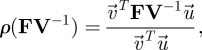
Define ρ(M) to be the spectral radius of matrix M (i.e. the maximum absolute value (or modulus) of all the eigenvalues).

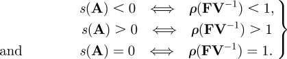
Next-generation theorem (van den Driessche & Watmough 2002). For any decomposition of the form A = F − V satisfying s(−V) < 0, V⁻¹ ≥ 0 and F ≥ 0,

2.2

Here, F ≥ 0 requires that all elements of F are greater than or equal to 0. The theorem can be understood graphically in the complex plane as a statement that all the eigenvalues of A have negative real parts, if and only if (denoted by ⟺) all the eigenvalues of FV⁻¹ lie within the unit circle.

Although the above theorem is phrased in terms of the properties of the eigenvalues of matrices, it has clear significance with respect to the above question of stability in dynamical systems. The conditions on the left-hand side are the ‘standard tool’ for assessing equilibrium stability, and the NGT allows one to replace these with alternative conditions. For many problems of biological interest, F and V can be chosen in a natural way to satisfy the conditions of the theorem (van den Driessche & Watmough 2002). Then, one essentially moves from the analysis of one eigenvalue problem involving s(A) to another involving ρ(FV⁻¹). The benefit of doing so is that the second problem is easier and provides meaningful biological information.

As an example, suppose is a vector representing the number of individuals in each of several classes in a structured population. Then we can usually find a biologically meaningful decomposition, A = F − V, where F is a matrix which gives the rate at which new individuals appear in class j, per individual of type i. Given this definition, all the elements of F are non-negative as required by the NGT. The matrix V describes the movement of existing individuals among the different classes, as well as the loss of these individuals. The system would eventually result in the loss of all individuals (owing to death) and, therefore, the other requirement for applying the NGT, s(−V) < 0, is also satisfied.

Given the above decomposition, the ijth element of the matrix FV⁻¹ then has a very useful interpretation; it is the expected lifetime number of type i individuals produced by a type j individual. In other words, the elements of FV⁻¹ represent the ‘generational’ output of type i by type j. Hence, FV⁻¹ is sometimes referred to as the next-generation matrix. Moreover, when F and V are chosen as described above, then ρ(FV⁻¹) = ℛ₀, which has an interpretation as the expected lifetime reproductive output of a newborn individual. Specific examples of how F and V can be chosen for evolutionary models are provided in §3.

Although the NGT is frequently used to determine the local stability of fixed points of ODEs like system (2.1), the proofs of the NGT use results from matrix theory such as the Perron–Frobenius theorem (Nold 1980, lemma 3.1; Diekmann & Heesterbeek 2000, theorem 6.13) or properties of singular and non-singular M-matrices (van den Driessche & Watmough 2002, theorem 2). To gain a better intuition for the NGT, it is helpful to view it explicitly in a dynamical systems context. Specifically, as we will outline next, we can view the theorem as a means of connecting the asymptotic dynamics of system (2.1) with an associated discrete-time recursion. The NGT sits at the interface between these two different ways of describing the same dynamical process.

To begin, from the statement of the NGT, equation (2.1) can be rewritten as

2.3

for F and V satisfying the requirements of the NGT. Now consider reformulating this as an infinite-dimensional system of ODEs

2.4

where 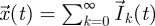, and with initial conditions and for all k ≥ 1. When F and V are chosen to be biologically meaningful, is an n-dimensional vector representing the number of ‘generation k’ individuals in each of the n classes. All future biological interpretations of quantities assume that F and V have been chosen in this way. The population starts with individuals in the different classes, and these individuals move around among classes (and are removed from the system) while producing ‘generation 1’ individuals in each of the classes (whose numbers are denoted by the vector ). These individuals then move around among the different classes (and are removed) while producing ‘generation 2’ individuals and so on. Here, a generation is defined as all the offspring of the previous generation.

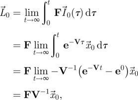
Now define 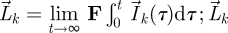is therefore an n-dimensional vector whose elements represent the total number of offspring that generation k individuals produce over all time, in each of the n classes. Integrating both sides of equation (2.4) from 0 to t and taking the limit t → ∞, we derive a recursive relation for

2.5

and therefore for all k > 0

2.6

where the final equality makes use of the fact that for all k (see the electronic supplementary material). Equation (2.6) tells us that the total number of offspring in each class that are produced by a particular generation changes by FV⁻¹ for every successive generation (also see Diekmann & Heesterbeek 2000, p. 74).

We can proceed further and solve the first differential equation in equation (2.4) to obtain . Therefore,

2.7

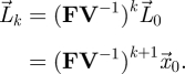
which uses the condition that s(−V) < 0. With this initial value of , we then arrive at the recursion

2.8

Therefore, from equation (2.1), which tells us how the number of individuals of all generations changes over time, we were able to derive equation (2.8), which tells us how the total offspring produced changes through successive generations. The NGT tells us that the number of individuals in all generations, , blows up over time if, and only if, the total number of offspring produced by a particular generation, , blows up as generations pass. In other words, the asymptotic dynamics of are governed by ρ(FV⁻¹), whereas the asymptotic dynamics of are governed by s(A), and the NGT theorem reveals that there is a strict correspondence between the two. Asymptotically, it takes a constant amount of time for the population to increase by a factor ρ(FV⁻¹) (i.e. de Camino-Beck & Lewis 2008), and therefore the NGT can be viewed as converting a continuous-time dynamical system to a discrete-time dynamical system that grows only when the original system grows. We note that the above manipulations are possible because F and V do not depend on time or generation number and that this is a necessary condition of the NGT.

As a final note, the connection between system (2.1) and its associated recursion (2.8) can be better appreciated by considering the case where x(t) is a scalar (and thus F and V are scalars). An explicit solution of equation (2.4) can then be found as I_k(t) = (Ft)^k e^−Vt (1/k!)x₀. Thus, the number of individuals in the kth generation, I_k (t), is proportional to a gamma probability density. The number of individuals in generation 1 increases until a time when births from generation 0 are too few to offset the mortality rate of the aging cohort (figure 1, equation (2.4)). The same is true of later generations, and this gives the number of generation k individuals for k > 1 a ‘hump’ shape as a function of time. Over successive generations, the plots form successive waves either growing in size or decaying depending upon whether F/V > 1 or F/V < 1, respectively (figure 1).

Figure 1.

(a)–(c) The number of individuals in each generation as a function of time was determined by numerically solving equation (2.4). The line originating at (0, 1) shows the size of the founding population decreasing exponentially. These panels show the temporal dynamics of the number of individuals in generation 1 (bold, solid), generation 2 (bold, long-dashed), generation 3 (bold, short-dashed) and all other generations in plain style lines. Parameter values are (a,d) F = 1 (all panels), V = 0.9; (b,e) V = 1; and (c,f) V = 1.1. (d,f) Show the temporal dynamics of the cumulative number of individuals in the 0–kth generation. In the lower left corner of (d)–(f), the founding population decreases exponentially. The top most line is the total number of individuals summed across all generations. (d) The population grows exponentially when F/V > 1, (e) remains unchanged when F/V = 1 and (f) decreases exponentially for F/V < 1. The bold solid line is the number of individuals in the founding and first generation. The bold long-dashed line is the number of individuals in the founding, first and second generation, and the bold short-dashed line is the number of individuals in the founding to third generation.

3. Evolutionary Invasion Analysis

Our next aim is to illustrate how the NGT can be used in evolutionary invasion analyses. Below, we present a series of three examples that build in complexity. The first example is simple enough that both the traditional approach and the NGT approach are equally easy to apply. This helps to illustrate the connection between the two. The second example then illustrates how the NGT approach can sometimes be substantially simpler than the traditional approach. Finally, the third example demonstrates how the NGT approach can be extended to even more complex models.

3.1. Example 1

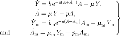
Consider a stage-structured population of juveniles (young), Y, and adults, A. Adults give birth to juveniles at a rate dependent on the density of adults. When A is near zero, the per capita birth rate is b and as A increases the per capita birth rate decreases at an exponential rate a owing to crowding. Juveniles mature at a constant rate, μ, and adults die at a constant rate, p. In a monomorphic population, the population dynamics are given by

3.1

where unless preceded by a negative sign each of the terms on the right-hand side is positive or zero. Let us now suppose that we are interested in the evolution of the birth, maturation and/or death rate, b, μ and p, respectively. Proceeding using the typical approach to evolutionary invasion analyses (Otto & Day 2007), we find the conditions for the system (3.1) reach a stable non-trivial equilibrium and then introduce a mutant with altered b, μ and/or p values. To do so, we augment system (3.1) to account for the mutant dynamics and modify the equations to reflect interactions between the mutants and individuals with the original trait (referred to as the resident trait). We will assume that the resident interacts with the mutant through crowding, which reduces the mutant birth rate. The mutant–resident system of equations is therefore

3.2

where Y_m and A_m denote the number of individuals with the mutant trait. The non-trivial resident equilibrium from equations (3.1) is therefore an equilibrium of equations (3.2) when Y_m = 0 and A_m = 0. The stability properties of this equilibrium of equations (3.2) tell us whether the mutant can invade or not.

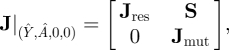
To examine the local stability of the mutant-free equilibrium, we obtain the Jacobian matrix of equations (3.2)

3.3

where the upper block, J_res, contains the partial derivatives of Ẏ and Ȧ with respect to Y and A, S contains the partial derivatives of Ẏ and Ȧ with respect to Y_m and A_m and the lower block (sometimes referred to as the mutant submatrix) is

3.4

The resident-only system is stable, and therefore s(J_res) < 0, for b > p. As J is a block diagonal matrix, the equilibrium (Ŷ, Â, 0, 0) is unstable when s(J_mut) > 0.

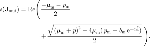
In this example, we can understand the evolution of the traits b_m, μ_m and p_m by the form of the interaction between residents and mutants. In equations (3.2), the density-dependent effect of resident individuals on the mutant birth rate is multiplicative. Therefore, we know that selection will maximize b_m/p_m (Mylius & Diekmann 1995, result 1). In this example, we show that this conclusion can be reached using either the traditional approach or next-generation methods. First, proceeding with the traditional approach, we calculate s(J_mut),

3.5

and the mutant invades if s(J_mut) > 0 and fails to invade if s(J_mut) < 0. The condition for mutant invasion looks complicated, but it can be reduced to

3.6

by using the Routh–Hurwitz criteria (Edelstein-Keshet 1998, §6.4) or by noting that only the correct sign of s(J_mut) is needed to correctly characterize invasibility. The final step is then to evaluate this expression at Â. There are two ways in which this might be done. First, we can solve for the equilibrium values directly from equations (3.1) to obtain  = (log(b) − log(p))/a, and then insert this into equation (3.5). Alternatively, we can use the fact that s(J_mut) = 0 when p_m = p and b_m = b because, in this case, the mutant is identical to the resident and thus should have neutral stability, and this property is used to eliminate the unknowns in equations (3.5). In either case, the final result is

3.7

This can be interpreted as the instantaneous growth rate of the mutant when the resident population is at equilibrium. The mutant will invade if s(J_mut) > 0, meaning that the mutant growth rate must be positive in the resident-only population. This occurs only if p_m/b_m > p/b.

We can now compare the above ‘traditional’ approach with one using the NGT. Everything proceeds exactly as above until the point where we have calculated the mutant submatrix, J_mut. Then, instead of calculating s(J_mut), we use the NGT to decompose J_mut into J_mut = F − V. To apply the NGT, all the elements of F must be non-negative and the maximum real parts of the eigenvalues of −V must be negative. Next, we discuss how F and V can be chosen for evolutionary models.

Recalling that the elements of F represent the appearance of new individuals, we return to equations (3.2) and determine for every term of every element of J_mut whether that term arose from a process describing the appearance of new individuals, or from a process describing the movement or death of existing individuals. In biological systems, new individuals appear as either births or immigration terms and all other terms are assigned to V. For models of parasite evolution, ‘births of the parasite’ refers to the appearance of newly infected hosts. Such terms are assigned to the F matrix. The movement of individuals usually refers to physical movement between spatial patches, maturation to a new life stage or progression to a more advanced type of disease. These terms as well as death and emigration terms are assigned to the V matrix.

Finally, there are some restrictions on the types of evolutionary models to which evolutionary invasion analyses of this type can be applied. The formal requirements on the nonlinear model are (A 1)–(A 5) in van den Driessche & Watmough (2002), and these can be simply recast in terms of evolutionary models by replacing ‘infectives’ with mutants. These requirements are needed so that J will be of the form described in equation (3.3) and are needed for both the traditional approach and the next-generation method. The most notable requirement is that immigration cannot occur at a constant rate. This is because constant immigration of mutants makes it unlikely that (Ŷ, Â, 0, 0) is a stable equilibrium of equations (3.2).

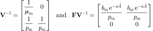
In equations (3.2) new individuals arise owing to the birth term in the Ẏ_m equation, the maturation of juveniles reflects the movement of individuals between states, and, therefore,

3.8

Here, the elements of V have the opposite sign as they do in equations (3.2) so that J_mut = F − V to satisfy the NGT. If we are not interested in the biological interpretation of ρ(FV⁻¹), then F and V can be chosen differently provided they satisfy the conditions of the NGT; the threshold condition for the mutant trait to invade, ρ(FV⁻¹) > 1, is equivalent for alternative decompositions (van den Driessche & Watmough 2002). For this decomposition, one can then readily calculate

3.9

Clearly, then,

3.10

The final step is to evaluate equation (3.10) at the mutant-free equilibrium. As with the traditional approach, there are two ways in which this might be done: we can solve for the equilibrium values directly as before or we can use the fact that ρ(FV⁻¹) = 1 when p_m = p and b_m = b to eliminate the unknowns in equation (3.10). Either way, we get

3.11

The mutant will invade if ρ(FV⁻¹) > 1, meaning that a single mutant in a resident population at equilibrium produces more than one new mutant during its lifetime. This condition can be seen as equivalent to the condition s(J_mut) > 0, as both correspond to the condition b_m/p_m > b/p.

3.2. Example 2

The above example is simple enough that the NGT does not afford any substantial advantage over the traditional approach. As the dimensionality of the model gets larger, however, the NGT can sometimes provide a much simpler analysis, as the following example illustrates.

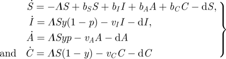
Consider an epidemiological model where S is the number of susceptible individuals and where, upon infection, three different types of diseases can occur: an acute infection, I, an autoimmune disease, A, or a chronic infection, C. Here, we view an autoimmune disease as occurring when lymphocytes that react with the parasite cross-react with host tissues. The parameter that determines the cross-reactivity of lymphocytes is p. The probability that the host produces lymphocytes specific for the infecting parasite is y. Here, we will consider the evolution of a host trait, y. A simple model for the epidemiological dynamics is

3.12

where Λ = β_I I + β_A A + β_C C (i.e. the force of infection), v_i is the per capita death rate owing to the disease of type i, b_i is the per capita birth rate of type i individuals and d is the per capita background mortality rate (figure 2). The parameter values for which equation (3.12) reaches a stable equilibrium can be determined numerically. We then introduce a mutant host type with an altered value of the trait y (denoted y_m). The augmented system, including the mutant, is then

3.13

and

3.14

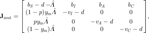
where the new force of infection is Λ = β_I (I + I_m) + β_A (A + A_m) + β_C (C + C_m). For equations (3.13), the matrix J_mut is

3.15

where 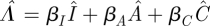. The characteristic polynomial is

where

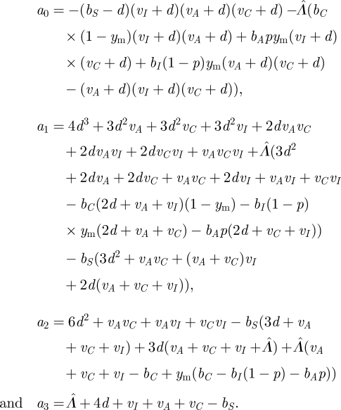Figure 2.

Susceptible individuals, S, can contract one of the three different diseases: an acute infection, I, an autoimmune disease, A, or a chronic infection, C. The per capita mortality rates for each of the diseases are v_C, v_A and v_I and the background mortality rate is d. The birth rates are b_S, b_I, b_A and b_C, respectively, and all newborns are susceptible. The host produces lymphocytes against the infection with probability y. The probability that the lymphocytes cross-react with host tissues causing an autoimmune disease is p. In §3.2, we derive the expression for fitness when a rare mutant with the trait y_m arises in the host population.

The traditional approach then requires one to determine the properties of the roots of this fourth-order polynomial. While such an analysis can sometimes be done (e.g. using the Routh–Hurwitz criteria), this approach clearly can rapidly become cumbersome.

The next-generation approach, however, is often much simpler. Under the interpretation of F and V given earlier, we decompose J_mut as

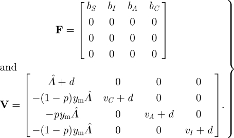3.16

Here, we are interested in host evolution, so the appearance of new individuals refers to the birth of new hosts. Note that s(−V) < 0 as v_C, v_A, v_I, d and Λ̂ are positive, and it is easy to check that the other conditions of the NGT are satisfied as well. The next-generation matrix is therefore

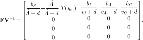3.17

where

is the number of expected offspring from a single infected individual. Therefore,

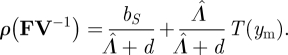3.18

Clearly, the NGT provides a much simpler approach to obtaining invasion conditions for this model than does the traditional analysis. Perhaps even more significantly, it also immediately provides an expression that has a clear and useful biological interpretation. The first term on the right-hand side of equation (3.18) represents the total reproductive output of a mutant host while susceptible, and the remaining term represents the expected total reproductive output of such a host once infected (each of these terms corresponds to one of the infection outcomes, weighted by its probability of occurrence). The mutant host type will therefore invade provided that the sum total of all this reproductive output is greater than 1.

To finish the analysis, we need to evaluate expression (3.18) at the mutant-free equilibrium. Although the equilibrium values of the variables can be obtained directly from system (3.12), the calculations are somewhat long and tedious. As mentioned in the previous example, however, we can instead use the fact that ρ(FV⁻¹) = 1 when y_m = y to greatly simplify matters. In particular, this reveals that

and therefore the expression for the mutant growth factor is

3.19

Here, ρ(FV⁻¹) = ℛ₀ because we chose biologically meaningful F and V. To interpret the expression for ℛ₀, it is best to consider equation (3.18). We also note that, at the mutant-free equilibrium, resident individuals affect the mutant through the scalar quantity, Λ. Therefore, there is no chance of a stable polymorphism for this model (Heino et al. 1998).

Before proceeding to the final example, it is useful to pause for a moment to consider why the NGT technique provides an easier approach in this example. Mathematically, the answer has to do with the forms of F and V in the decomposition. If we define F and V as discussed in §2, then frequently F has only one row with non-zero elements. As a result, the matrix FV⁻¹ will be upper triangular even though the original matrix F − V need not be. This makes it easier to evaluate the eigenvalues of FV⁻¹ than those of F − V.

From a biological standpoint, the fact that F has only one row with non-zero elements means that new individuals are always born into a single class. This is typically the case for age- and stage-structured models, but it is often true in other forms of population structure as well. For example, with infectious diseases, new infections often arise in only one class (e.g. exposed, but uninfectious individuals) and then move into other classes afterwards. In either case, one can think of a typical new individual as being the one that starts in this ‘newborn’ class. We then simply imagine following this individual throughout its lifetime, adding up all of the new individuals that it produces in this newborn class. The resulting quantity is simply ρ(FV⁻¹), which is the lifetime reproductive output of a newly formed mutant individual.

3.3. Example 3

The above example illustrates that, when all new individuals enter the model through a single class, the NGT typically provides a very simple and biologically meaningful approach to conducting evolutionary invasion analyses. In this final example, we will demonstrate that, even when new individuals enter the model through more than one class, the NGT approach can still be useful. In such cases, the matrix FV⁻¹ will no longer be upper triangular, and thus finding its eigenvalues need no longer be any easier than finding those of F − V. Nevertheless, working in terms of FV⁻¹ can still have its advantages in terms of providing biological insight. We will work primarily with a two-dimensional system to simplify the presentation, but the same principles hold in higher dimensions as well.

Before getting into the details of a specific example, let us first consider some general remarks. Starting with the matrix FV⁻¹, an elementary result of matrix analysis shows that

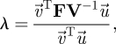3.20

where and are the left and right eigenvectors of FV⁻¹ associated with the eigenvalue λ. As FV⁻¹ ≥ 0, the Perron–Frobenius theorem tells us that the eigenvalue of maximum modulus is real (Seneta 1973) and therefore

3.21

where and are the eigenvectors associated with the leading eigenvalue. The elements of the left eigenvector are proportional to the reproductive values of each type of individual, and the elements of the right eigenvector are proportional to the equilibrium numbers of each type. Furthermore, we can choose these eigenvectors in such a way that .

Now, let us consider the 2 × 2 case with eigenvectors normalized so that . We have

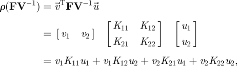3.22

where K_ij is the ijth element of the next-generation matrix, and corresponds to the expected lifetime number of type i individuals produced by a single type j individual. Recall that, in the previous example, where all newborns entered through a single class, we made no use of the concept of reproductive value. Now, however, because newborns can enter through multiple classes, we need to convert these newborns of different classes into a common currency. The reproductive values, v_i, do this for us. They allow us to compare the value of producing newborns in each of the different classes.

Given these considerations, we can interpret equation (3.22) as the sum of contributions from each stage in the stage-structured population. For example, grouping terms by u_i, we have

3.23

The first term in equation (3.23) accounts for the contribution of type 1 individuals. Here, the fraction of individuals that are of type 1 is u₁, each of which produces a total of K₁₁ type 1 offspring during their lifetime (with type 1 offspring having a value of v₁), as well as a total of K₂₁ type 2 individuals (with type 2 offspring having a value of v₂). Likewise, the second term accounts for type 2 individuals' contributions. If the sum total of these contributions is greater than 1, then invasion will occur.

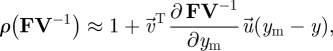
Equation (3.23) provides a useful biological interpretation of the invasion fitness, but, as already mentioned, when the time to actually calculate this expression explicitly comes, it is no easier than working with the original matrix F − V. The reason is that, even though the elements of the matrix FV⁻¹ can sometimes be relatively easy to derive, the eigenvectors and are also functions of the elements of this matrix. Nevertheless, in many evolutionary invasion analyses, we can still use the NGT to make easy progress because we are often interested in mutant trait values that are very close to the resident trait value (i.e. mutations of small effect). In such cases, we can approximate ρ(FV⁻¹) as

3.24

where all terms of equation (3.24) are evaluated at y_m = y (see the electronic supplementary material). Equation (3.24) is often relatively easy to evaluate because the eigenvectors are now calculated for the special case where y_m = y, and the matrix ∂FV⁻¹/∂y_m involves only differentiating the elements of FV⁻¹.

We now illustrate these ideas using an example of a spatially structured population. Consider a population subdivided into two patches with migration of newborns between patches. The question of interest is this: if there is a trade-off between adaptation to patch 1 versus patch 2, how do the demographic dynamics affect the way this trade-off is resolved?

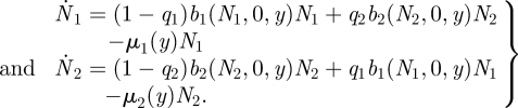
Define N₁ and N₂ as the population size of the resident phenotype in each patch. Suppose that a fraction, q_i, of the new births in patch i migrate to the other patch and vice versa. Assume that births are density dependent (within a patch) and use b_i (N_i, N_im, y) to denote the per capita birth rate. Density dependence in the birth rate is due to competition for resources, but the fraction of newborns that migrate is a constant. Use μ_i (y) as the per capita death rate where y is an underlying trait that mediates the trade-off in adaptation to each patch. The model for the resident-only system is then

3.25

Next, we suppose the necessary conditions for this system to reach a stable non-trivial equilibrium have been determined and we introduce a mutant genotype with an altered value of y (denoted y_m). The augmented system is as above but with b_i(N_i, N_im, y), plus the same equations for the mutant

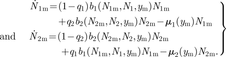3.26

The mutant submatrix for this model is

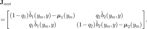3.27

where we have suppressed some arguments of functions for notational simplicity (e.g. we are using b̃_i (y_m, y) to denote b_i(0, N̂_i, y_m), where N̂_i is the equilibrium value of the resident population in patch i and the dependence of b̃_i (y_m, y) on y is because N̂_i is a function y). The traditional approach would then calculate s(J_mut), which can be readily done by solving for the roots of the characteristic polynomial of J_mut using the quadratic formula. Note, however, that the resulting expression is not particularly easy to interpret.

The next-generation approach first calculates FV⁻¹, giving

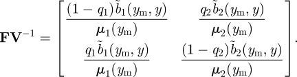3.28

The ijth element of the matrix (3.28) is the number of new patch i offspring produced over the lifespan of a patch j individual. Using formula (3.23) for ρ(FV⁻¹), we have

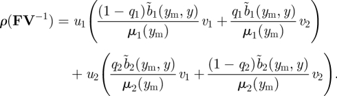3.29

Thus, invasion fitness can be viewed as the sum of contributions from patch 1 and patch 2. The first term is the number of offspring produced by a patch 1 mutant that stay on patch 1, plus that number of offspring produced by a patch 1 mutant that move to patch 2 (each weighted by the appropriate reproductive value). The fraction of such mutant individuals on patch 1 is u₁. The second term can be interpreted analogously.

To proceed further, if we assume that the mutant trait value is close to that of the resident, we can then use approximation (3.24). In this case, when y = y_m we have and . Therefore, equation (3.24) gives

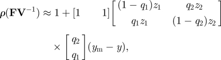3.30

where the z_i are selection gradients defined as

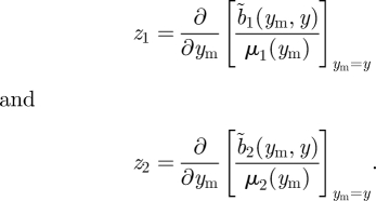Expression (3.30) simplifies to

3.31

Therefore, invasion fitness depends on the weighted sum of the selection gradient, z_i, in each patch. The approximation (3.31) illustrates that, when q₂ is larger than q₁, selection favours adaptation to patch 1. This makes sense as migration to patch 1 exceeds migration away from patch 1 when q₂ > q₁.

4. Summary

The quantity ℛ₀ has been called ‘one of the most important concepts in epidemic theory’ (Heesterbeek & Dietz 1996; Heffernan et al. 2005), as it provides a natural way to characterize the potential for an infectious disease to spread. Not surprisingly then, researchers have sought various ways to simplify the calculation of this quantity. Next-generation methods (Diekmann et al. 1990; Diekmann & Heesterbeek 2000; van den Driessche & Watmough 2002) have become one of the most important tools in this regard, because they provide a convenient way to perform such calculations. Other related approaches have recently been developed based on graph-theoretical techniques (de Camino-Beck et al. 2008).

Given that the NGT essentially provides a simplified way for performing some linear stability analyses, it is not surprising that this approach might also be useful in the context of evolutionary invasion analyses. Although a few authors have employed this approach, it is vastly underutilized. The purpose of this review is to bring this technique to a broader evolutionary audience, by providing an intuitive connection between it and the more traditional approach in evolutionary invasion analyses (§2), and by illustrating its utility through a series of three examples (§3).

In §2, we illustrated that, when dealing with the stability properties of a linear system of ODEs, one can derive an associated recursion where the increase in population size owing to the contribution of a generation corresponds to an equivalent increase in the population by all generations over some discrete-time step. The original system of differential equations models how the number of individuals of all generations changes over time, whereas the associated recursion models how the number of offspring produced by a generation over all time changes through successive generations. The key result of the NGT is that the number of individuals of all generations expands over time if, and only if, the number of offspring produced by a particular generation also expands as generations pass. Given that the former system essentially quantifies the dynamics in terms of real time, whereas the latter does so in terms of numbers of generations, this correspondence makes good intuitive sense.

In §3, we then illustrated how the NGT can sometimes make evolutionary invasion analyses simpler. In particular, this approach often offers a substantial advantage whenever new individuals are always born into a single class. In this case, we typically find that the next-generation matrix, FV⁻¹, is triangular, thereby making the calculation of its eigenvalues easy. From a biological point of view, the dominant eigenvalue of this matrix can be viewed as the lifetime reproductive output of a newly introduced individual. Such an interpretation is straightforward because all such offspring always enter in the same class.

When new individuals are not always born into the same class, the NGT typically does not yield much mathematical advantage and the approach is not often used in this context in mathematical epidemiology. Nevertheless, we have also demonstrated in §3 that the approach can still be of considerable value in this case, particularly in the context of evolutionary invasion analyses. First, it provides a very helpful form for invasion fitness that can be easily interpreted, even when the ensuing calculations are difficult. Second, because we are often interested in small mutational steps in evolutionary invasion analyses, it can also provide some helpful mathematical machinery.

Taken together, the above considerations demonstrate that next-generation methods can be a very useful way to approach evolutionary invasion analyses. Certainly, it will not always make such analyses easier, but it provides an important additional tool to have at one's disposal, especially when dealing with models of high dimension.

References

- Abrams P. A. 2001. Modelling the adaptive dynamics of traits involved in inter- and intraspecific interactions: an assessment of three methods. Ecol. Lett. 4, 166–175. ( 10.1046/j.1461-0248.2001.00199.x) [DOI] [Google Scholar]
- Abrams P. A., Matsuda H., Harada Y. 1993. Evolutionarily unstable fitness maxima and stable fitness minima of continuous traits. Evol. Ecol. 7, 465–487. ( 10.1007/BF01237642) [DOI] [Google Scholar]
- Alizon S., Hurford A., Mideo N., van Baalen M. 2009. Virulence evolution and the trade-off hypothesis: history, current state of affairs and future. J. Evol. Biol. 22, 245–259. ( 10.1111/j.1420-9101.2008.01658.x) [DOI] [PubMed] [Google Scholar]
- Anderson R. M., May R. M. 1982. Coevolution of hosts and parasites. Parasitology 85, 411–426. ( 10.1017/S0031182000055360) [DOI] [PubMed] [Google Scholar]
- Boldin B. 2006. Introducing a population into a steady community: the critical case, the center manifold and the direction of the bifurcation. SIAM J. Appl. Math. 66, 1424–1453. ( 10.1137/050629082) [DOI] [Google Scholar]
- de Camino-Beck T., Lewis M. A. 2008. On net reproductive rate and the timing of reproduction output. Am. Nat. 172, 128–139. ( 10.1086/588060) [DOI] [PubMed] [Google Scholar]
- de Camino-Beck T., Lewis M. A., van den Driessche P. 2008. Graph-theoretic method for the basic reproduction number in continuous time epidemiological models. J. Math. Biol. 59, 503–516. ( 10.1007/s00285-008-0240-9) [DOI] [PubMed] [Google Scholar]
- Diekmann O., Heesterbeek J. A. P. 2000. Mathematical epidemiology of infectious diseases: model building analysis and interpretation. Chichester, UK: John Wiley and Sons Inc. [Google Scholar]
- Diekmann O., Heesterbeek J. A. P., Metz J. A. J. 1990. On the definition and computation of the basic reproduction ratio R0 in models for infectious diseases in heterogeneous populations. J. Math. Biol. 28, 365–382. ( 10.1007/BF00178324) [DOI] [PubMed] [Google Scholar]
- Dieckmann U., Law R. 1996. The dynamical theory of coevolution. J. Math. Biol. 34, 579–612. ( 10.1007/BF02409751) [DOI] [PubMed] [Google Scholar]
- Edelstein-Keshet L. 1998. Mathematical models in biology. New York, NY: The Random House. [Google Scholar]
- Eshel I. 1983. Evolutionary and continuous stability. J. Theor. Biol. 103, 99–111. ( 10.1016/0022-5193(83)90201-1) [DOI] [PubMed] [Google Scholar]
- Frank S. A. 1996. Models of parasite virulence. Q. Rev. Biol. 71, 37–78. ( 10.1086/419267) [DOI] [PubMed] [Google Scholar]
- Geritz S. A. H., Kisdi É., Meszéna G. 1998. Evolutionarily singular strategies and the adaptive growth and branching of the evolutionary tree. Evol. Ecol. 12, 35–37. ( 10.1023/A:1006554906681) [DOI] [Google Scholar]
- Gyllenberg M., Metz J. A. J. 2001. On fitness in structured metapopulations. J. Math. Biol. 43, 545–560. ( 10.1007/s002850100113) [DOI] [PubMed] [Google Scholar]
- Hamilton W. D. 1967. Extraordinary sex ratios. Science 156, 477–488. ( 10.1126/science.156.3774.477) [DOI] [PubMed] [Google Scholar]
- Heesterbeek J. A. P., Dietz K. 1996. The concept of R0 in epidemic theory. Stat. Neerl. 50, 89–110. ( 10.1111/j.1467-9574.1996.tb01482.x) [DOI] [Google Scholar]
- Heffernan J. M., Smith R. J., Wahl L. M. 2005. Perspectives on the basic reproductive ratio. J. R. Soc. Interface 2, 281–293. ( 10.1098/rsif.2005.0042) [DOI] [PMC free article] [PubMed] [Google Scholar]
- Heino M., Metz J. A. J., Kaltala V. 1998. The enigma of frequency-dependent selection. TREE 13, 367–370. [DOI] [PubMed] [Google Scholar]
- Maynard Smith J. 1982. Evolution and the theory of games. Cambridge, UK: Cambridge University Press. [Google Scholar]
- Maynard Smith J., Price G. R. 1973. Logic of animal conflict. Nature 246, 15–18. ( 10.1038/246015a0) [DOI] [Google Scholar]
- Metz J. A. J., Nisbet R. M., Geritz S. A. H. 1992. How should we define ‘fitness’ for general ecological scenarios? TREE 7, 198–202. ( 10.1098/rspb.2000.1373) [DOI] [PubMed] [Google Scholar]
- Mylius S. D., Diekmann O. 1995. On evolutionarily stable life histories, optimization and the need to be specific about density dependence. Oikos 74, 218–224. ( 10.2307/3545651) [DOI] [Google Scholar]
- Nold A. 1980. Heterogeneity in disease-transmission modeling. Math. Biosci. 52, 227–240. ( 10.1016/0025-5564(80)90069-3) [DOI] [Google Scholar]
- Otto S. P., Day T. 2007. Evolutionary invasion analysis. In A biologist's guide to mathematical modeling in ecology and evolution, pp. 454–502. Princeton, NJ: Princeton University Press. [Google Scholar]
- Reed J., Stenseth N. C. 1984. On evolutionary stable strategies. J. Theor. Biol. 108, 491–508. ( 10.1016/S0022-5193(84)80075-2) [DOI] [Google Scholar]
- Seneta E. 1973. Non-negative matrices: an introduction to theory and applications. London, UK: George Allen and Unwin. [Google Scholar]
- Taylor P. D. 1989. Evolutionary stability in one-parameter models under weak selection. Theor. Pop. Biol. 36, 125–143. ( 10.1016/0040-5809(89)90025-7) [DOI] [Google Scholar]
- van Baalen M. 1998. Coevolution of recovery ability and virulence. Proc. R. Soc. Lond. B 265, 317–325. ( 10.1098/rspb.1998.0298) [DOI] [PMC free article] [PubMed] [Google Scholar]
- van den Driessche P., Watmough J. 2002. Reproduction numbers and sub-threshold endemic equilibria for compartmental models of disease transmission. Math. Biosci. 180, 29–48. ( 10.1016/S0025-5564(02)00108-6) [DOI] [PubMed] [Google Scholar]