

Abstract
Understanding the risk of airborne transmission can provide important information for designing safe healthcare environments with an appropriate level of environmental control for mitigating risks. The most common approach for assessing risk is to use the Wells–Riley equation to relate infectious cases to human and environmental parameters. While it is a simple model that can yield valuable information, the model used as in its original presentation has a number of limitations. This paper reviews recent developments addressing some of the limitations including coupling with epidemic models to evaluate the wider impact of control measures on disease progression, linking with zonal ventilation or computational fluid dynamics simulations to deal with imperfect mixing in real environments and recent work on dose–response modelling to simulate the interaction between pathogens and the host. A stochastic version of the Wells–Riley model is presented that allows consideration of the effects of small populations relevant in healthcare settings and it is demonstrated how this can be linked to a simple zonal ventilation model to simulate the influence of proximity to an infector. The results show how neglecting the stochastic effects present in a real situation could underestimate the risk by 15 per cent or more and that the number and rate of new infections between connected spaces is strongly dependent on the airflow. Results also indicate the potential danger of using fully mixed models for future risk assessments, with quanta values derived from such cases less than half the actual source value.
Keywords: airborne infection, ventilation, Wells–Riley, stochastic, hospital
1. Introduction
Airborne transmission of infectious diseases is a subject of increasing interest driven by a wide range of factors including: greater understanding of the role played by indoor air and ventilation provision in the dispersal and transport mechanisms of a wide range of pathogens; changing expectations of hospital patients, particularly in developed countries; and the emergence of new or drug-resistant disease strains with the potential to spread on a global scale. Tuberculosis (TB) is an archetypal example of a disease that is transmitted by a true airborne route; primary infection occurs when droplet nuclei containing Mycobacterium tuberculosis bacilli are inhaled. These tiny particles (typically <5 µm in diameter) can remain suspended in the air for long periods of time with local airflow pathways inside a building determining their fate. TB is a particular concern as it is once again a worldwide health problem, compounded by the increased susceptibility to M. tuberculosis in HIV/AIDS patients, ease of world travel and the increased prevalence of multidrug-resistant tuberculosis (MDR-TB). Specialist ventilation and isolation facilities are recommended to control nosocomial (hospital) spread (Siegel et al. 2007) and those on the front line advocate secondary environmental control measures such as ultraviolet germicidal irradiation to further minimize risk (Nardell et al. 1991; Escombe et al. 2009). Although excluded from the medical definition of airborne infection, the transmission of disease by pathogen-contaminated droplets also involves transport through the air. The emergence of severe acute respiratory syndrome (SARS) in 2002–2003 caused a global health scare (Riley et al. 2003), with the causative agent, a highly infectious coronavirus (Lipsitch et al. 2003), thought to be primarily spread through localized contact with contaminated droplets. However, there is evidence that individuals were apparently infected without sufficiently close contact with a known case (Scales et al. 2003), and retrospective studies of building airflow patterns suggested that airborne dispersal may play a significant role (Li et al. 2005). In recent months, the potential for a global influenza pandemic has created similar anxieties for those tasked with controlling wide-scale disease spread. Again the infection is linked to droplet transmission and the time scale for production of a vaccine and limitations of drug treatment mean that physical and procedural control strategies are the primary defence against widespread transmission (Morse et al. 2006).
Although many nosocomial infections are primarily associated with direct person-to-person contact, there is considerable evidence that aerial dissemination of pathogens may play an important role in many hospital-acquired infections. In recent years airborne transmission has been implicated in nosocomial outbreaks of Staphylococcus aureus (Farrington et al. 1990; Mertens 1996) and Acinetobacter spp. (Allen & Green 1987; Kumari et al. 1998) as well as many viral outbreaks. The high secondary attack rates seen in norovirus outbreaks have also been attributed to the dispersion droplets, released when patients vomit, that rapidly evaporate to form airborne droplet nuclei and are distributed by air currents around hospitals. With hospital design and operation in the developed world now driven by infection control targets and increasingly the energy use agenda, better understanding of the relationships between the design of the physical environment and the risk of infection is becoming increasingly essential in establishing robust guidance for those charged with developing and managing healthcare facilities. This paper reviews the application of the Wells–Riley model for relating the risk of airborne infection to parameters in the indoor environment and the developments applied to address some of the limitations in the original model. A stochastic formulation is presented which is coupled with a simple zonal ventilation model to demonstrate the role of airflow and population size on the risk of infection and the implications for design, risk assessment and future research.
2. Modelling airborne infection
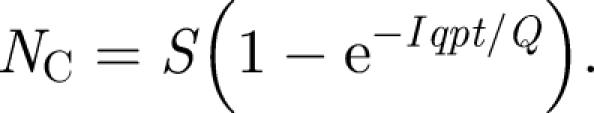
Transmission of infection is a complex process at the best of times with the risk of disease determined by numerous factors that have considerable and uncertain variability including: the characteristics of the pathogen concerned, the infectiousness of the host, the media in which it is passed from source to new host and the immune response of the new host. Transmission through airborne routes complicates this further by adding the influence of building airflows to the process. Despite this, researchers in epidemiology have developed a range of approaches for modelling disease dynamics from the classic models such as Susceptible-Infector-Susceptible (SIS) and Susceptible-Infector-Removed (SIR) models, which make use of average rate coefficients to describe progression of a disease in a population (Bailey 1957) to more recent studies based on dose–response data (Jones et al. 2009) or that incorporate the pathogen–host biological interaction (Chen et al. 2009). Much of the previous research quantifying airborne infection rates in confined spaces has stemmed from the work of Wells (1955) and Riley et al. (1978), using the analytical expression known as the Wells–Riley equation. This relates the number of infective (I) and susceptible (S) people in a space, the room ventilation rate (Q, m3 s−1) and the quantity of infectious material in the air to predict the number of new cases infected, NC, over a period of time t (s):
 |
2.1 |
Here p (m3 s−1) is the pulmonary ventilation rate of susceptible individuals, while q represents a unit of infection termed as ‘quantum’, introduced by Wells (1955), to express the response of susceptible individuals to inhaling infectious droplet nuclei. He postulated that not all inhaled droplet nuclei will result in infection and defined a quantum of infection as the number of infectious droplet nuclei required to infect 1 − 1/e susceptible people. The term quantum or quanta of infection is widely used in evaluating airborne infections and is usually interpreted as a measure that effectively indicates both the quantity and virulence of infectious material present in the air.
Numerous researchers have carried out risk-analysis studies based on this model including the evaluation of personal protective equipment (Gammaitoni & Nucci 1997), tuberculosis risk in buildings (Nardell et al. 1991) and the dispersion of Bacillus anthracis from envelopes (Fennelly et al. 2004). The study conducted by Gammaitoni & Nucci (1997) also showed a fundamental formulation of the Wells–Riley equation that enables transient ventilation effects to be included. An earlier study reviewing Wells–Riley type models (Beggs et al. 2003) highlighted that although the models give useful indications of expected transmission in a wide range of circumstances, their simple nature results in several limitations described here.
2.1. Disease dynamics
The original Wells–Riley formulation is confined to only predicting new cases of a disease, an assumption that is valid where the incubation period (or time for a new case to become infective) is longer than the time scale of the model. With the model most commonly used to evaluate TB transmission, this is generally justified as the incubation is typically weeks or even years, and (with the exception of long-term confinement such as prisons), occupants are generally not in contact longer than the incubation period. The assumption is also valid for short incubation period diseases if the model is applied over very short time scales, such as transmission of influenza on an aircraft as considered by Rudnick & Milton (2003). However, in the case of transmission of diseases such as influenza, SARS or norovirus in hospitals, which may have an airborne component to the transmission, the time scale of contact is comparable to the incubation period and therefore the dynamics of the disease must be considered. It is straightforward to extend the model to include the long-term dynamics of an infection by coupling with classic epidemic models as described in Noakes et al. (2006a). Such an approach enables both the disease and environmental parameters to be explored, allowing the combined role of nursing behaviour with controls such as ventilation, personal protective equipment or vaccination (Chen & Liao 2008) to be assessed through a single model. Interestingly, the original paper first describing the Wells–Riley equation (Riley et al. 1978) applied it to a measles outbreak in a school, a disease and setting that do not meet the above criteria. To accommodate this the authors applied the model over discrete time periods, using the cases and susceptibles at the end of each period as the initial conditions for the next period rather than coupling with an epidemic model.
2.2. Population size
One of the key limitations with the Wells–Riley model concerns the small size of populations in hospital environments and the role that chance effects play in determining infection risk. Equation (2.1) is based on the Poisson law of small chances, which assumes that in a small enough time period only one new infection is likely. This is suitable for most airborne infections where it is easy to define a time period that approximates to this criterion. However, although the Wells–Riley model is derived from this probabilistic approach, it is more commonly used in deterministic simulations, with equation (2.1) used to predict average infection risk in different scenarios. In particular, the model has been used successfully in studies to examine both the impact of interventions on the progression of an infection, as well as retrospectively to find the average quanta production rate from outbreak data, particularly relating to TB transmission. Treating the model as one describing a deterministic process is only strictly suitable for large populations, and to understand the variability in risk for small numbers, such as hospital patients, it is necessary to apply the model in a stochastic simulation.
2.3. Proximity
The Wells–Riley model assumes that the air is well mixed leading to a uniform concentration of bioaerosols throughout the space. This is rarely true even in spaces with the best designed ventilation systems and therefore does not account for the influence of proximity between infective and susceptible people. In particular this is an issue when analysing the risk of infection in a space consisting of connected rooms, such as hospital wards. This can be partially addressed by using zonal ventilation or computational fluid dynamics (CFD) modelling techniques to simulate the airflow and dispersion of contaminants, revealing regions of good and poor mixing and areas of high contaminant concentrations that would constitute a higher risk to occupants. Zonal or network ventilation models are well used in evaluating ventilation flows in large multi-connected spaces such as whole buildings. While they are limited in that they are not capable of resolving local details of airflows and are less well suited to large spaces such as atria (Mora et al. 2003), they have been shown to give good prediction of bulk air movement and contaminant transport in a range of applications including natural ventilation (Asfour & Gadi 2007) and particle dispersion (Hu et al. 2007). Two of the most widely used models, COMIS and CONTAM, were developed by national laboratories in the USA and are used in both research and design applications (Chen 2009). Zonal modelling has previously been applied to airborne infection risk, including simulation of ultraviolet disinfection (Noakes et al. 2004a) showing good comparison to CFD models and studies by Ko et al. (2004) and Jones et al. (2009) considering TB transmission on an airliner. Ko et al.'s study used both a fully mixed model as well as approximating the spatial variation by dividing the airliner cabin into four zones with incomplete mixing between zones. Combining this with the Wells–Riley model and spatial distribution data from a real outbreak enabled them to show that compartmentalization of airflow in cabins acts to limit transmission of any infection throughout the entire aircraft. Jones et al. (2009) also adopted a zonal approach, dividing the aircraft into 34 zones with the ventilation and interzonal flows based on measured data with results indicating spatial transmission patterns dependent on the turbulent mixing between zones. CFD offers a strategy for modelling the detailed spatial distribution of pathogens in indoor environments. A number of recent studies have considered hospital applications (Chow & Yang 2004; Noakes et al. 2006b) or bioaerosol dispersal (Noakes et al. 2004b), and the 2003 SARS outbreak generated a lot of interest using CFD to model the spread of contagion within and between buildings (Yu et al. 2004; Li et al. 2005). A recent paper (Qian et al. 2009) has linked CFD simulations and the Wells–Riley model with results showing correlation between predicted and observed spatial infection risk. Despite the details available from CFD modelling, using the technique to simulate airflow in large multi-connected buildings requires significant computational resources that are unavailable or inappropriate in many cases. A recent review by Chen (2009) highlights a move towards the use of ‘coarse grid’ CFD and coupling CFD models to zonal ventilation models to provide higher levels of accuracy without excessive computational effort.
2.4. Infectious dose
Perhaps the biggest limitation with the Wells–Riley model is the representation of the infectious dose through the expression ‘quantum’ of infection. While this is a simple approach that is easily analogous to the concentration of a pathogen in the air, the single parameter cannot fully capture the complex interaction between infectors, pathogens and potential hosts that occurs in reality. As highlighted in Pujol et al. (2009), the Wells–Riley model is only appropriate for infections that can be modelled with an exponential dose–response where a single large dose can be considered to be the same as the equivalent in smaller doses over a longer time period. As such the model cannot incorporate the immune system response that may act to control pathogens arriving at low doses over a long time period and is likely to be inappropriate for estimating risk at low doses (Haas 1983). Nicas & Hubbard (2002) also recognize this limitation and go on to suggest that the Wells–Riley model is only strictly valid where infection is initiated by a single micro-organism and the quanta represents the risk of this being inhaled and initiating infection. The model has been most widely applied to TB, which is believed to satisfy these criteria (Escombe et al. 2007); however, it may be less appropriate for many other infections, especially where the infectious dose is low (Nicas & Hubbard 2002). Recent research is starting to develop strategies to address these weaknesses through the application of disease-specific characteristics and dose–response data, much of which has developed through risk assessment of pathogens in water and wastewater (Haas 1983; Mara et al. 2007). Studies focusing on airborne transmission include Armstrong & Haas (2007a,b) who outline a framework for using quantitative microbial risk assessment (QMRA) in modelling the risk of legionnaire's disease, using dose–response data from animal studies. Bartrand et al. (2008) consider a similar approach in the transmission of B. anthracis, again through fitting distribution models to published non-human dose–response data, while Jones et al.'s (2009) study also uses a QMRA approach in evaluating M. tuberculosis transmission. Chen et al. (2009) adopt a slightly different approach, using a Wells–Riley framework to describe global parameters, but linking both viral kinetics and the characteristics of exhaled bioaerosols to incorporate the disease characteristics in the transmission of influenza. The most recent studies in this area (Huang & Haas 2009; Pujol et al. 2009) are building on these dose–response model developments to consider the risk over time from single or multiple doses, enabling the immune response seen in reality to be incorporated into analyses. Although the primary interest in this paper is on the environmental parameters rather than the disease characteristics, these recent developments clearly offer a valuable strategy for understanding the role of pathogen–human interaction in disease transmission and are likely to play a key role in future model developments.
3. Stochastic zonal model
By considering equation (2.1) an infection rate λ can be written as
 |
3.1 |
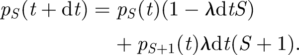
A stochastic formulation of the Wells–Riley equation is based on the probability that there are S uninfected susceptibles at time t, pS(t) = Pr(S susceptibles at time t). In a small time interval, dt, such that the probability of more than one infection is negligible, two outcomes are possible: one new infection with probability λ dtS or no new infection with probability 1 − λ dtS. Therefore, the process can be expressed as
 |
3.2 |
As dt tends to zero, this yields the differential equation
 |
3.3 |
This can be solved using a numerical approach in which the process is considered to consist of a series of infection events where the susceptible population decreases by one in each case. As shown by Renshaw (1991), for a population of S susceptibles and a disease that can be approximated by an exponential dose–response, the time T to the next event is an exponentially distributed random variable with
| 3.4 |
This can be used to simulate the time to the next event, t, using a random number 0 ≤ Y ≤ 1 by the equation
 |
3.5 |
With λ defined by equation (3.1, the result in equation (3.5) can be easily applied to derive a series of inter-event times corresponding to the new cases of infection among the susceptible population in a ventilated indoor environment.
To account for the proximity of an infector to susceptibles and the incomplete mixing in interconnected ward spaces, the above model is applied within a zonal ventilation model. Here the air within each zone is treated as uniformly mixed; however, the mixing between the zones is limited. The infectious quanta is treated as a deterministic variable leading to a concentration distribution throughout the ward space. A simplified approach is applied which represents a realistic spatial arrangement of a ward but uses fixed interzonal ventilation rates to model transfer into and out of zones rather than environment-specific pressure coefficients. It must be highlighted that this approach is used only to demonstrate the behaviour of the stochastic risk model in a multi-zone space and the results are a considerable simplification of reality. However, it is straightforward to apply the approach described here using any ventilation network model or CFD simulation to assess the spatial distribution of infectious material in a real situation.
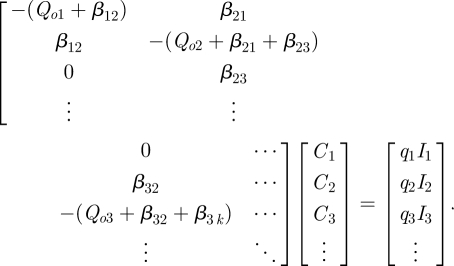
For the general case shown schematically in figure 1, the concentration of infectious material in the ith zone Ci can be approximated by considering the generation, ventilation removal and interzonal transfers for each case to give
 |
3.6 |
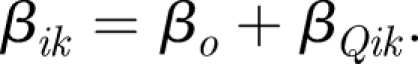
Here, the term qiIi represents the generation rate in the zone, Qoi is the extract ventilation rate in zone i and βik and βki represent the volume flow rate of air to and from adjacent zones k, respectively. These interzonal flow rate terms consist of two components: a global mixing rate βo which is a constant value in both directions across all zonal boundaries in the model plus an additional component βQik which expresses the net flow across a boundary owing to a ventilation imbalance between the two zones (Brouns & Waters 1991). This component is specific to the ventilation system and is defined for each boundary in the model to give the total interzonal flow rate as
 |
3.7 |
Figure 1.

Schematic representation of simple zonal model for three adjacent zones. Solid black arrows indicate ventilation extract, solid grey arrows indicate interzonal flows, dashed black arrows indicate infection source within the zone.
Under steady-state conditions, equation (3.6) is equal to zero for each zone and yields a set of equations that can be represented in matrix form and solved through a Gaussian elimination technique. This is shown partially below for the simple schematic case in figure 1:
 |
3.8 |
The infection risk model is made zone dependent by replacing the term qI/Q with the zone concentration Ci from the solution of equation (3.8), giving
| 3.9 |
As the new infection may now occur in any one of the occupied zones within the model, it is necessary to examine the relative probability of infection in each to determine in which zone each infection event occurs. At each time step, the probability that the next infection event will be in zone i is given by
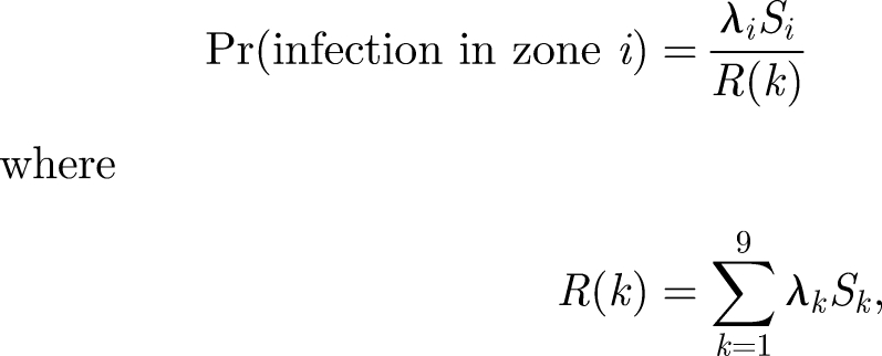 |
3.10 |
with the inter-event time now given by
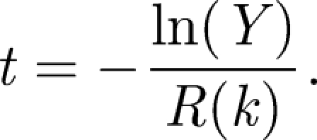 |
3.11 |
The numerical simulation of this process again follows the methodology described by Renshaw (1991)
(i) Calculation of λiSi/R(k) for each zone at the current time step.
(ii) Generation of a first random number 0 ≤ Y ≤ 1 to find the inter-event time.
(iii) Generation of a second random number 0 ≤ X ≤ 1 to establish which zone is infected based on infection in zone 1 if 0 ≤ X ≤ λ1S1/R(k), zone 2 if λ1S1/R(k) ≤ X≤λ2S2/R(k), etc.
(iv) Change Si to Si−1 in infected zone i.
The model was implemented using Excel and VBA (Microsoft) incorporating a Monte Carlo approach to enable each model to run up to 100 times to calculate mean behaviour and the s.d. As the equations are defined in terms of inter-event times, which are different in every simulation owing to the random number in the event time definition, it was necessary to map each result onto a regular time scale in order to be able to find average data across more than one simulation. The simulations were mapped onto a 170 h time period divided into hourly steps, then plotted every 3 h to enable the data to be seen clearly.
4. Results
The models described above were used to investigate the influence of population and airflows on the risk of infection through a parametric study approach. The model was based on a hypothetical hospital ward layout as shown in figure 2 comprising three identical six-bedded bays that open out onto a common corridor. To investigate a range of possible ventilation scenarios, each bay is divided into two equal zones (each containing three occupants) and the corridor split into three equal zones corresponding to the adjacent ward. The model assumes that ventilation air can be supplied and/or extracted from each zone and there is some degree of mixing between adjacent zones that is influenced by the ventilation regime as described above. All cases simulated a ward occupancy of 18 patients (six per bay) of which one located in zone 1a was assumed to be infectious. All patients were equally susceptible and breathed the ward air at a constant rate of 0.01 m3 min−1 (10 l min−1). Six different ventilation regimes were investigated as detailed in table 1 to explore the effect of directional airflow. Although these specified different supply and extract volumes to the various zones, the total ventilation rate over the whole ward was 27 m3 min−1 in all cases, equivalent to an average air change rate of 3 AC h−1.
Figure 2.

Hypothetical ward layout used in the study showing possible ventilation supply/extract (black arrows) and interzonal mixing (grey arrows).
Table 1.
Volume flow rate in and out of each zone for the six ventilation regimes.
| regime | zones 1a, 2a, 3a |
zones 1b, 2b, 3b |
zones c1, c2, c3 |
|||
|---|---|---|---|---|---|---|
| supply (m3 min−1) | extract (m3 min−1) | supply (m3 min−1) | extract (m3 min−1) | supply (m3 min−1) | extract (m3 min−1) | |
| A | 3 | 3 | 3 | 3 | 3 | 3 |
| B | 9 | 0 | 0 | 0 | 0 | 9 |
| C | 0 | 9 | 0 | 0 | 9 | 0 |
| D | 6 | 6 | 0 | 0 | 3 | 3 |
| E | 6 | 0 | 0 | 6 | 3 | 3 |
| F | 0 | 6 | 6 | 0 | 3 | 3 |
The interzone mixing parameter βo was constant across all zone boundaries with a value between 9 and 27 m3 min−1 depending on the simulation. The ventilation-dependent component of the interzone mixing βQik was defined to simulate directional airflow induced by a ventilation regime.
The final parameter is the value of quanta generation, which is particularly difficult to define for most infections. Previous researchers have estimated the values from outbreak data using equation (2.1) and the actual number of new cases. Most of the values given in the literature relate to TB outbreaks and the data collated in Beggs et al. (2003) indicate that for most pulmonary TB cases, a generation rate of between 1.25 and 60 quanta h−1 can be assumed. Higher values of hundreds or even thousands of quanta per hour are associated with medical procedures, such as bronchoscopy or abscess irrigation where the generation rate of infectious aerosols is increased. Riley et al. (1978) calculated a value of 570 quanta h−1 for a school measles outbreak, while Rudnick & Milton (2003) estimated quanta production rates for rhinovirus as 1–10 quanta h−1 and influenza as 15–128 quanta h−1. For the purposes of this study, a quanta production rate of 0.5 quanta min−1 (30 quanta h−1) is used. As the aim of this study is to examine the relative impact of the occupant and airflow parameters on the risk of infection, the actual quanta production rate is not critical. However, we will return to the definition and calculation of quanta in §5, as the model results raise some important questions about estimating quanta, and hence risk, from equation (2.1).
4.1. Stochastic effects
Prior to considering the effect of ventilation parameters, figures 3 and 4 compare the zonal and stochastic behaviour with a fully mixed deterministic simulation using equation (2.1) for a single infector generating 30 quanta h−1. Figure 3 compares both approaches for the fully mixed case, presented in terms of a mean value with error bars indicating 1 s.d. In the stochastic model this is based on the data from 100 simulations, while in the deterministic solution, mean and s.d. are based on the Poisson assumption used in the derivation of equation (2.1). As such, the number of cases is taken as the Poisson mean and s.d. as the square root of the mean. As expected, the mean values from both the models are almost identical and both show considerable variability in the mean result. However, the expected variance differs between approaches, with a similar range predicted after short time duration, but a greater deviation from the mean indicated by the deterministic solution over a longer time period. This difference is probably apparent because basing the variability on the mean value from the deterministic solution inherently assumes variability in all parameters of the model, while the variation in the stochastic solution is due solely to the small population.
Figure 3.

Comparison of variability from mean results in stochastic and deterministic fully mixed models. Error bars show 1 s.d. from the mean, with grey capped error bars for the stochastic model and black uncapped error bars for the deterministic model.
Figure 4.

Effect of air mixing on the total rate of infection. Error bars show 1 s.d. from the mean value. Solid line denotes βo = 27 m3 min−1; open triangle denotes βo = 9 m3 min−1; filled diamond denotes fully mixed.
In figure 4, the deterministic fully mixed mean is compared with the zonal model results for ventilation regime A and the infector located in zone 1a. In this case all zones have an equal supply and extract volume flow rate; therefore, the interzonal mixing is solely due to the value of βo, with no additional transfer through ventilation imbalance (βQik = 0). Results presented show the effect of air mixing on the total number of new cases across the whole ward. With a value of βo = 9 m3 s−1, the overall infection rate is much slower than the fully mixed model, with less than two-thirds of the predicted total number of cases after the 170 h time period. Increasing the mixing to βo = 27 m3 s−1 increases the rate at which the infection spreads with now around 85 per cent of the fully mixed model. The figure again shows the considerable variability in a small population with considerable overlap between the range of results for the two mixing parameters and a deviation of approximately ±15 per cent from the mean value in either stochastic simulation.
4.2. Effect of airflow paths
Although the results in figure 4 provide some initial insight into the potential influence of ventilation, the air mixing between the rooms is not influenced by the ventilation regime in this case. To understand the potential impact of this, simulations are run for all six ventilation regimes in table 1 using a fixed value of βo = 9 m3 s−1. In all cases, Monte Carlo simulations are performed with 100 simulation runs to yield mean infection rates for each of the three ward bays. The results from these simulations are presented in figure 5 in terms of infection risk, where a risk of one is equivalent to all six patients in a bay being infected.
Figure 5.

Effect of ventilation regime on the risk of infection over a 170 h period. Mean data obtained from 100 simulation runs. (a) Infections in bay 1. (b) Infections in bay 2. (c) Infections in bay 3. Filled diamonds, case A; open squares, case B; filled triangles, case C; crosses, case D; open triangles, case E; open diamonds, case F.
The results in figure 5 demonstrate both the influence of proximity and ventilation flows on the risk of infection for patients on the ward over time. As expected, the risk of infection in bay 1 (figure 5a), where the infector is located, is much higher than the other two bays, with the ventilation regime having little impact on the risk. Although ventilation regime C suggests a slightly lower infection rate compared with the other five regimes, the risk is still over 90 per cent over the 170 h period. The results for the other two bays (figure 5b,c), however, clearly demonstrate the potential impact of the ventilation system on the risk of airborne pathogen transfer throughout the space. In both cases, even with the stochastic variability in the data, the risk of infection is highest with ventilation regime D and lowest with regime C, with the risk around 50 per cent lower in bay 2 and 60 per cent lower in bay 3.
5. Discussion
The results presented above give some initial insight into both the variability of infection risk likely to be present in real situations as well as the role that ventilation flows may play in the transmission of infection.
The results in figures 3 and 4 clearly show that considering the stochastic variation produces a considerably wider range of predicted cases than the mean result typically derived from deterministic simulations. The model presented here indicates that the actual number of new infections could deviate from the mean by up to two cases owing to chance effects in a small population alone. As the results in figure 3 indicate, if there is uncertainty in other parameters, this could result in an even wider deviation. While the Wells–Riley model is a very straightforward approach for carrying out assessments as part of outbreak planning, the deterministic mean has the potential to significantly underestimate the bed numbers, staffing and resources needed to respond to an outbreak. As such some level of stochastic variability should be taken into account when using Wells–Riley type models in this way.
Hospital ventilation is typically designed on a mixing ventilation approach with little consideration beyond provision of adequate comfort except in certain applications such as isolation rooms, units for immunosuppressed patients or operating theatres. Although the zonal model presented here is a very simple representation of ventilation flows and is limited as a model of a real situation, the results do give some qualitative indication of the importance of airflow paths between zones in the transmission of infection. Many of the results are intuitive as can be seen by presenting the worst (D) and best (C) cases schematically in figure 6. In case C the air pathways are from the corridor to the ward, reducing the risk of airborne pathogens generated within a particular bay being transferred to other bays by extracting from the source location. However, in case D (and also cases A and E), the ventilation provides little or no additional movement of potential pathogens within the space. Although this does not actively promote the transfer between spaces, at the same time it does nothing to restrict it with little directional flow to limit transfer into other areas. These findings suggest that some approaches could be inadvertently contributing to the spread of infection and that careful design of a system could potentially provide greater protection for patients within a hospital ward.
Figure 6.

Schematic of ventilation flows in regimes D and C. Location of infector indicated by star. Black arrows indicate ventilation flow; grey arrows indicate interzonal mixing flows.
The results presented in figure 5a suggest that case C also has some advantage in reducing within-bay transmission; however, this result should be treated with a good deal of caution. The results presented are the mean results from 100 stochastic simulations. The variability in the data plus the uncertainty over the exact location of the infector in the ward implies that, in reality, it is difficult to say from this model how the ventilation system impacts on the risk within a single bay. To understand the level of risk in this case more detailed simulations of the airflow, such as CFD analysis, are essential to show how the location of ventilation supply and extract vents influences the risk of cross-infection between patients (Noakes et al. 2006b).
Apart from giving some insight into the role of the ventilation system, the model applied above raises some important issues relating to the assessment of risk in indoor environments and use of quanta values in such activities. Regardless of the ventilation regime and layout, these results show a clear dependence of risk on the proximity to the infector. As shown by figure 5, with the values used in this hypothetical study patients in the same space as the infector have over a 90 per cent risk of infection over the 170 h period, while those two bays away (bay 3) have less than a 35 per cent risk over the same period. However, most quanta values quoted in the literature are calculated from outbreak data and do not consider the influence of proximity. The assumed value of 30 quanta h−1 with ventilation case A in the zonal stochastic model resulted in a mean number of infections across the whole ward of 10.2 in the 170 h period.
Quanta values presented in the literature take the total number of infections over a period of time, assume complete mixing and manipulate equation (2.1) to find the value for quanta production. In this case, using 10.2 new cases, 17 susceptibles in a fully mixed space with a total ventilation rate of 27 m3 min−1 over 170 h, this yields a quanta production rate of 14.5 quanta h−1, less than half the actual value. This suggests that using a fully mixed model to determine quanta production rates from outbreak data may significantly underestimate the quanta values in environments such as multi-zoned hospital wards or office buildings where the air will be far from fully mixed. In addition, using such values derived from outbreaks to estimate risk and design control procedures may significantly underestimate the actual risk, particularly for susceptible people in closer proximity to the index case. Although shown here from a simple representation of the ventilation, the results concur with the findings of Qian et al. (2009) who showed differences between quanta values determined from mixed and spatially varying CFD models.
6. Conclusions
The Wells–Riley model has been used to examine airborne infectious disease transmission since the 1970s and remains a simple and valuable approach for understanding the role of various parameters to inform research, design and risk assessment. Linking the model with ventilation flows is a straightforward and practical option for those involved in the design and risk assessment of healthcare buildings. Provided users appreciate the limitations of the Wells–Riley model and their ventilation model, the approach enables a much greater understanding of the possible spatial transmission of infection and allows design and operational control strategies to be explored. The importance of stochastic effects, especially in small populations, should not be underestimated and users should seek to incorporate this into any model to evaluate the potential range of risk.
Coupling the model with disease dynamics, vaccination and environmental control strategies have also been tackled in previous studies and shown to give greater insight into the role of environmental and management strategies, particularly for the transmission of short incubation period diseases. The greatest uncertainty in the Wells–Riley model remains the disease parameters, with the concept of quanta suitable for parametric studies but severely limited in real risk assessments owing to the necessity to derive expected values from prior outbreaks. However, recent developments are showing considerable promise for establishing new methodologies for evaluating airborne disease transmission based on the dose–response characteristics of real pathogens. While this is currently limited by available time–dose data relevant to human subjects (Pujol et al. 2009), the right collaboration between those conducting experimental dosing studies and the infection risk modelling community could significantly enhance knowledge of disease characteristics and the pathogen–host interaction. Linking such knowledge to models incorporating environmental parameters offers a very effective framework for future assessment of airborne disease transmission in indoor environments.
Acknowledgements
The authors would like to acknowledge the support of the Department of Health, Estates and Facilities Division Research and Development Fund in funding this study.
Footnotes
One contribution of 10 to a Theme Supplement ‘Airborne transmission of disease in hospitals’.
References
- Allen K. D., Green H. T. 1987. Hospital outbreak of multi-resistant Acinetobacter anitratus: an airborne mode of spread? J. Hosp. Infect. 9, 110–119. ( 10.1016/0195-6701(87)90048-X) [DOI] [PubMed] [Google Scholar]
- Armstrong T. W., Haas C. N. 2007a. A quantitative microbial risk assessment model for Legionnaires' disease: animal model selection and dose-response modelling. Risk Anal. 27, 1581–1596. ( 10.1111/j.1539-6924.2007.00990.x) [DOI] [PubMed] [Google Scholar]
- Armstrong T. W., Haas C. N. 2007b. Quantitative microbial risk assessment model for Legionnaires' disease: assessment of human exposures for selected spa outbreaks. J. Occup. Environ. Hyg. 4, 634–646. ( 10.1080/15459620701487539) [DOI] [PubMed] [Google Scholar]
- Asfour O. S., Gadi M. B. 2007. A comparison between CFD and network models for predicting wind-driven ventilation in buildings. Build. Environ. 42, 4079–4085. ( 10.1016/j.buildenv.2006.11.021) [DOI] [Google Scholar]
- Bailey N. T. 1957. The mathematical theory of epidemics. London, UK: Griffin & Co. [Google Scholar]
- Bartrand T. A., Weir M. H., Haas C. N. 2008. Dose-response models for inhalation of Bacillus anthracis spores: interspecies comparisons. Risk Anal. 28, 1115–1124. ( 10.1111/j.1539-6924.2008.01067.x) [DOI] [PubMed] [Google Scholar]
- Beggs C. B., Noakes C. J., Sleigh P. A., Fletcher L. A., Siddiqi K. 2003. The transmission of tuberculosis in confined spaces: an analytical study of alternative epidemiological models. Int. J. Tuberc. Lung Dis. 7, 1015–1026. [PubMed] [Google Scholar]
- Brouns C., Waters B. 1991. A guide to contaminant removal effectiveness. AIVC technical note 28.2, Air Infiltration and Ventilation Centre, Belgium. [Google Scholar]
- Chen Q. 2009. Ventilation performance prediction for buildings: a method overview and recent applications. Build. Environ. 44, 848–858. ( 10.1016/j.buildenv.2008.05.025) [DOI] [Google Scholar]
- Chen S. C., Liao C. M. 2008. Modelling control measures to reduce the impact of pandemic influenza among schoolchildren. Epidemiol. Infect. 136, 1035–1045. [DOI] [PMC free article] [PubMed] [Google Scholar]
- Chen S. C., Chio C. P., Jou L. J., Liao C. M. 2009. Viral kinetics and exhaled droplet size affect indoor transmission dynamics of influenza infection. Indoor Air 19, 401–413. ( 10.1111/j.1600-0668.2009.00603.x) [DOI] [PubMed] [Google Scholar]
- Chow T. T., Yang X. Y. 2004. Ventilation performance in the operating theatre against airborne infection: review of research activities and practical guidance. J. Hosp. Infect. 56, 85–93. ( 10.1016/j.jhin.2003.09.020) [DOI] [PubMed] [Google Scholar]
- Escombe A. R., et al. 2007. The detection of airborne transmission of tuberculosis from HIV-infected patients using an in vivo air sampling model. Clin. Infect. Dis. 44, 1349–1357. ( 10.1086/515397) [DOI] [PMC free article] [PubMed] [Google Scholar]
- Escombe A. R., et al. 2009. Upper-room ultraviolet light and negative air ionization to prevent tuberculosis transmission. PLoS Med. 6, e1000043 ( 10.1371/journal.pmed.1000043) [DOI] [PMC free article] [PubMed] [Google Scholar]
- Farrington M., Ling J., Ling T., French G. L. 1990. Outbreaks of infection with methicillin-resistant Staphylococcus aureus on neonatal and burns units of a new hospital. Epidemiol. Infect. 105, 215–228. ( 10.1017/S0950268800047828) [DOI] [PMC free article] [PubMed] [Google Scholar]
- Fennelly K. P., Davidow A. L., Miller S. L., Connell N., Ellner J. J. 2004. Airborne infection with Bacillus anthracis: from mills to mail. Emerg. Infect. Dis. 10, 996–1001. [DOI] [PMC free article] [PubMed] [Google Scholar]
- Gammaitoni L., Nucci M. C. 1997. Using a mathematical model to evaluate the efficacy of TB control measures. Emerg. Infect. Dis 3, 335–342. ( 10.3201/eid0303.970310) [DOI] [PMC free article] [PubMed] [Google Scholar]
- Haas C. N. 1983. Estimation of risk due to low doses of microorganisms: a comparison of alternative methodologies. Am. J. Epidemiol. 118, 1097–1100. [DOI] [PubMed] [Google Scholar]
- Hu B., Freihaut J. D., Bahnfleth W. P., Aumpansub P., Thran B. 2007. Modeling particle dispersion under human activity disturbance in a multizone indoor environment. J. Arch. Eng. 13, 187–193. ( 10.1061/(ASCE)1076-0431(2007)13:4(187)) [DOI] [Google Scholar]
- Huang Y., Haas C. N. 2009. Time-dose-response models for microbial risk assessment. Risk Anal. 29, 648–661. ( 10.1111/j.1539-6924.2008.01195.x) [DOI] [PubMed] [Google Scholar]
- Jones R. M., Masago Y., Bartrand T. A., Haas C. N., Nicas M., Rose J. B. 2009. Characterizing the risk of infection from Mycobacterium tuberculosis in commercial passenger aircraft using quantitative microbial risk assessment. Risk Anal. 29, 355–365. ( 10.1111/j.1539-6924.2008.01161.x) [DOI] [PubMed] [Google Scholar]
- Ko G., Thompson K. M., Nardell E. A. 2004. Estimation of tuberculosis risk on a commercial airliner. Risk Anal. 24, 379–388. ( 10.1111/j.0272-4332.2004.00439.x) [DOI] [PubMed] [Google Scholar]
- Kumari D. N. P., Haji T. C., Keer V., Hawkey P. M., Duncanson V., Flower E. 1998. Ventilation grilles as a potential source of methicillin-resistant Staphylococcus aureus causing an outbreak in an orthopaedic ward at a district general hospital. J. Hosp. Infect. 39, 127–133. ( 10.1016/S0195-6701(98)90326-7) [DOI] [PubMed] [Google Scholar]
- Li Y., Huang X., Yu I. T. S., Wong T. W., Qian H. 2005. Role of air distribution in SARS transmission during the largest nosocomial outbreak in Hong Kong. Indoor Air 15, 83–95. ( 10.1111/j.1600-0668.2004.00317.x) [DOI] [PubMed] [Google Scholar]
- Lipsitch M., et al. 2003. Transmission dynamics and control of severe acute respiratory syndrome. Science 300, 1966–1970. ( 10.1126/science.1086616) [DOI] [PMC free article] [PubMed] [Google Scholar]
- Mara D. D., Sleigh P. A., Blumenthal U. J., Carr R. M. 2007. Health risks in wastewater irrigation: comparing estimates from quantitative microbial risk analyses and epidemiological studies. J. Water Health 5, 39–50. ( 10.2166/wh.2006.055) [DOI] [PubMed] [Google Scholar]
- Mertens R. A. F. 1996. Methodologies and results of national surveillance. Bailliere's Clin. Infect. Dis. 3, 159–178. [Google Scholar]
- Mora L., Gadgil A. J., Wurtz E. 2003. Comparing zonal and CFD model predictions of isothermal indoor airflows to experimental data. Indoor Air 13, 77–85. ( 10.1034/j.1600-0668.2003.00160.x) [DOI] [PubMed] [Google Scholar]
- Morse S. S., Garwin R. L., Olsiewski P. J. 2006. Next flu pandemic: what to do until the vaccine arrives? Science 314, 929 ( 10.1126/science.1135823) [DOI] [PubMed] [Google Scholar]
- Nardell E. A., Keegan J., Cheney S. A., Etkind S. C. 1991. Airborne infection: theoretical limits of protection achievable by building ventilation. Am. Rev. Resp. Dis. 144, 302–306. [DOI] [PubMed] [Google Scholar]
- Nicas M., Hubbard A. 2002. A risk analysis for airborne pathogens with low infectious doses: application to respirator selection against Coccidioides immitis spores. Risk Anal. 22, 1153–1163. ( 10.1111/1539-6924.00279) [DOI] [PubMed] [Google Scholar]
- Noakes C. J., Beggs C. B., Sleigh P. A. 2004a. Modelling the performance of upper room ultraviolet germicidal irradiation devices in ventilated rooms: comparison of analytical and CFD methods. Indoor Built Environ. 13, 477–488. ( 10.1177/1420326X04049343) [DOI] [Google Scholar]
- Noakes C. J., Fletcher L. A., Beggs C. B., Sleigh P. A., Kerr K. G. 2004b. Development of a numerical model to simulate the biological inactivation of airborne microorganisms in the presence of ultraviolet light. J. Aerosol Sci. 35, 489–507. ( 10.1016/j.jaerosci.2003.10.011) [DOI] [Google Scholar]
- Noakes C. J., Beggs C. B., Sleigh P. A., Kerr K. G. 2006a. Modelling the transmission of airborne infections in enclosed spaces. Epidemiol. Infect. 134, 1082–1091. ( 10.1017/S0950268806005875) [DOI] [PMC free article] [PubMed] [Google Scholar]
- Noakes C. J., Sleigh P. A., Escombe A. R., Beggs C. B. 2006b. Use of CFD analysis in modifying a TB ward in Lima, Peru. Indoor Built Environ. 15, 41–47. ( 10.1177/1420326X06062364) [DOI] [Google Scholar]
- Pujol J. M., Eisenberg J. E., Haas C. N., Koopman J. S. 2009. The effect of ongoing exposure dynamics in dose response relationships. PLoS Comp. Biol. 5, e1000399 ( 10.1371/journal.pcbi.1000399) [DOI] [PMC free article] [PubMed] [Google Scholar]
- Qian H., Li Y. G., Nielsen P. V., Huang X. H. 2009. Spatial distribution of infection risk of SARS transmission in a hospital ward. Build. Environ. 44, 1651–1658. ( 10.1016/j.buildenv.2008.11.002) [DOI] [Google Scholar]
- Renshaw E. 1991. Modelling biological populations in space and time (eds Cannings C., Hoppensteadt F. C., Segel L. A.). Cambridge, UK: Cambridge University Press. [Google Scholar]
- Riley E. C., Murphy G., Riley R. L. 1978. Airborne spread of measles in a suburban elementary school. Am. J. Epidemiol. 107, 421–432. [DOI] [PubMed] [Google Scholar]
- Riley S., et al. 2003. Transmission dynamics of the etiological agent of SARS in Hong Kong: impact of public health interventions. Science 300, 1961–1966. ( 10.1126/science.1086478) [DOI] [PubMed] [Google Scholar]
- Rudnick S. N., Milton D. K. 2003. Risk of airborne infection transmission estimated from carbon dioxide concentration. Indoor Air 13, 237–245. ( 10.1034/j.1600-0668.2003.00189.x) [DOI] [PubMed] [Google Scholar]
- Scales D. C., et al. 2003. Illness in intensive care staff after brief exposure to severe acute respiratory syndrome. Emerg. Infect. Dis. 9, 1205–1210. [DOI] [PMC free article] [PubMed] [Google Scholar]
- Siegel J. D., Rhinehart E., Jackson M., Chiarello L. Healthcare Infection Control Practices Advisory Committee. 2007. Guideline for isolation precautions: preventing transmission of infectious agents in healthcare settings. See http://www.cdc.gov/ncidod/dhqp/pdf/isolation2007.pdf. [DOI] [PMC free article] [PubMed] [Google Scholar]
- Wells W. F. 1955. Airborne contagion and air hygiene. Cambridge, MA: Harvard University Press. [Google Scholar]
- Yu I. T. S., Li Y. G., Wong T. W., Tam W., Chan A. T., Lee J. H. W., Leung D. Y. C., Ho T. 2004. Evidence of airborne transmission of the severe acute respiratory syndrome virus. N. Engl. J. Med. 350, 1731–1739. ( 10.1056/NEJMoa032867) [DOI] [PubMed] [Google Scholar]