Towards programming languages for genetic engineering of living cells

Abstract

Synthetic biology aims at producing novel biological systems to carry out some desired and well-defined functions. An ultimate dream is to design these systems at a high level of abstraction using engineering-based tools and programming languages, press a button, and have the design translated to DNA sequences that can be synthesized and put to work in living cells. We introduce such a programming language, which allows logical interactions between potentially undetermined proteins and genes to be expressed in a modular manner. Programs can be translated by a compiler into sequences of standard biological parts, a process that relies on logic programming and prototype databases that contain known biological parts and protein interactions. Programs can also be translated to reactions, allowing simulations to be carried out. While current limitations on available data prevent full use of the language in practical applications, the language can be used to develop formal models of synthetic systems, which are otherwise often presented by informal notations. The language can also serve as a concrete proposal on which future language designs can be discussed, and can help to guide the emerging standard of biological parts which so far has focused on biological, rather than logical, properties of parts.

1. Introduction

Synthetic biology aims at designing novel biological systems to carry out some desired and well-defined functions. It is widely recognized that such an endeavour must be underpinned by sound engineering techniques, with support for abstraction and modularity, in order to tackle the complexities of increasingly large synthetic systems (Endy 2005; Andrianantoandro et al. 2006; Marguet et al. 2007). In systems biology, formal languages and frameworks with inherent support for abstraction and modularity have long been applied, with success, to the modelling of protein interaction and gene networks, thus gaining insight into the biological systems under study through computer analysis and simulation (Garfinkel 1968; Sauro 2000; Regev et al. 2001; Chabrier-Rivier et al. 2004; Danos et al. 2007; Fisher & Henzinger 2007; Ciocchetta & Hillston 2008; Mallavarapu et al. 2009). However, none of these languages readily capture the information needed to realize an ultimate dream of synthetic biology, namely the automatic translation of models into DNA sequences which, when synthesized and put to work in living cells, express a system that satisfies the original model.

In this paper, we introduce a formal language for Genetic Engineering of living Cells (GEC), which allows logical interactions between potentially undetermined proteins and genes to be expressed in a modular manner. We show how GEC programs can be translated into sequences of genetic parts, such as promoters, ribosome binding sites and protein coding regions, as categorized for example by the MIT Registry of Standard Biological Parts (http://partsregistry.org). The translation may in general give rise to multiple possible such devices, each of which can be simulated based on a suitable translation to reactions. We thereby envision an iterative process of simulation and model refinement where each cycle extends the GEC model by introducing additional constraints that rule out devices with undesired simulation results. Following completion of the necessary iterations, a specific device can be chosen and constructed experimentally in living cells. This process is represented schematically by the flow chart in figure 1.

Figure 1.

Flow chart for the translation of GEC programs to genetic devices, where each device consists of a set of part sequences. The GEC code describes the desired properties of the parts that are needed to construct the device. The constraints are resolved automatically to produce a set of devices that exhibit these properties. One of the devices can then be implemented inside a living cell. Before a device is implemented, it can also be compiled to a set of chemical reactions and simulated, in order to check whether it exhibits the desired behaviour. An alternative device can be chosen, or the constraints of the original GEC model can be modified based on the insights gained from the simulation.

The translation assumes a prototype database of genetic parts with their relevant properties, together with a prototype database of reactions describing known protein–protein interactions. A prototype tool providing a database editor, a GEC editor and a GEC compiler has been implemented and is available for download (Pedersen & Phillips 2009). Target reactions are described in the Language for Biochemical Systems (Pedersen & Plotkin 2008), allowing the reaction model to be extended if necessary and simulated. Stochastic and deterministic simulation can be carried out directly in the tool (relying on the Systems Biology Workbench (Bergmann & Sauro 2006)) or through third-party tools after a translation to Systems Biology Markup Language (Hucka et al. 2003; Bornstein et al. 2008).

To our knowledge, only one other formally defined programming language for genetic engineering of cells is currently available, namely the GenoCAD language (Cai et al. 2007), which directly comprises a set of biologically meaningful sequences of parts. Another language is currently under development at the Sauro Lab, University of Washington. While GenoCAD allows a valid sequence of parts to be assembled directly, the Sauro Lab language allows this to be done in a modular manner and additionally provides a rich set of features for describing general biological systems. GEC also employs a notion of modules, but allows programs to be composed at higher levels of abstraction by describing the desired logical properties of parts; the translation deduces the low-level sequences of relevant biological parts that satisfy these properties, and the sequences can then be checked for biological validity according to the rules of the GenoCAD language.

Section 2 describes our assumptions about the databases, and gives an informal overview of GEC through examples and two case studies drawn from the existing literature. Section 3 gives a formal presentation of GEC through an abstract syntax and a denotational semantics, thus providing the necessary details to reproduce the compiler demonstrated by the examples in the paper. Finally, §4 points to the main contributions of the paper and potential use of GEC on a small scale, and outlines the limitations of GEC to be addressed in future work before the language can be adopted for large-scale applications.

2. Results

2.1. The databases

The parts and reaction databases presented in this paper have been chosen to contain the minimal structure and information necessary to convey the main ideas behind GEC. Technically, they are implemented in Prolog, but their content is informally shown in tables 1 and 2. The reaction table represents reactions in the general form enzymes ^∼ reactants→{r} products, optionally with some parts omitted as in the reaction luxI ^∼ →{1.0} m3OC6HSL, in which m3OC6HSL is synthesized by luxI. We stress that the mass action rate constants {r} are hypothetical, and that specific rates have been chosen for the sake of clarity. The last four lines of the reaction database represent transport reactions, where m3OC6HSL→[m3OC6HSL] is the transport of m3OC6HSL into some compartment.

Table 1.

Table representation of a minimal parts database. (The three columns describe the type, identifier and properties associated with each part.)

type	id	properties
pcr	c0051	codes(clR, 0.001)
pcr	c0040	codes(tetR, 0.001)
pcr	c0080	codes(araC, 0.001)
pcr	c0012	codes(lacI, 0.001)
pcr	c0061	codes(luxI, 0.001)
pcr	c0062	codes(luxR, 0.001)
pcr	c0079	codes(lasR, 0.001)
pcr	c0078	codes(lasI, 0.001)
pcr	cunknown3	codes(ccdB, 0.001)
pcr	cunknown4	codes(ccdA, 0.1)
pcr	cunknown5	codes(ccdA2, 10.0)
prom	r0051	neg(clR, 1.0, 0.5, 0.00005)
		con(0.12)
prom	r0040	neg(tetR, 1.0, 0.5, 0.00005)
		con(0.09)
prom	i0500	neg(araC, 1.0, 0.000001, 0.0001)
		con(0.1)
prom	r0011	neg(lacI, 1.0, 0.5, 0.00005)
		con(0.1)
prom	runknown2	pos(lasR-m3OC12HSL, 1.0, 0.8, 0.1)
		pos(luxR-m3OC6HSL, 1.0, 0.8, 0.1)
		con(0.000001)
rbs	b0034	rate(0.1)
ter	b0015

Table 2.

A minimal reaction database consisting of basic reactions, enzymatic reactions with enzymes preceding the ^∼ symbol and transport reactions with compartments represented by square brackets. (Mass action rate constants are enclosed in braces.)

luxR+m3OC6HSL→{1.0} luxR−m3OC6HSL

luxR−m3OC6HSL→{1.0} luxR+m3OC6HSL

lasR+m3OC12HSL→{1.0} lasR−m3OC12HSL

lasR−m3OC12HSL→{1.0} lasR+m3OC12HSL

luxI ∼→{1.0} m3OC6HSL

lasI ∼→{1.0} m3OC12HSL

ccdA ∼ ccdB→{1.0}

ccdA2 ∼ ccdB→{0.00001}

m3OC6HSL→{1.0} [m3OC6HSL]

m3OC12HSL→{1.0} [m3OC12HSL]

[m3OC6HSL]→{1.0} m3OC6HSL

[m3OC12HSL]→{1.0} m3OC12HSL

The parts table contains three columns, the first representing part types, the second representing unique IDs (taken from the Registry of Standard Biological Parts when possible) and the third representing sets of properties. For the purpose of our examples, the available types are restricted to promoters prom, ribosome binding sites rbs, protein coding regions pcr and terminators ter. Table 3 shows the set of parts currently available in GEC, together with their corresponding graphical representation. The shapes are inspired by the MIT registry of parts. The variables X, which occur as prefixes to part names and as labels in the graphical representation, range over part identifiers and will be discussed further in §2.2.

Table 3.

Parts in GEC with their corresponding graphical representation.

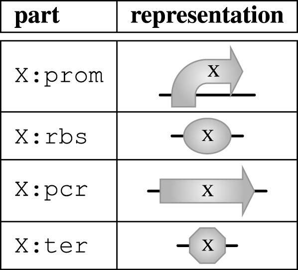Promoters can have properties pos(P,RB,RUB,RTB) and neg(P,RB,RUB,RTB), where P is a transcription factor (a protein or protein complex) resulting in positive or negative regulation, respectively. The remaining entries give a quantitative characterization of promoter regulation: RB and RUB are the binding and unbinding rates of the transcription factor to the promoter; and RTB is the rate of transcription in the bound state. Promoters can also have the property con(RT), where RT is the constitutive rate of transcription in the absence of transcription factors. Protein coding regions have the single property codes(P,RD) indicating the protein P they code for, together with a rate RD of protein degradation. Ribosome binding sites may have the single property rate(R), representing a rate of translation of mRNA.

While the reaction database explicitly represents reactions at the level of proteins, the rate information associated with the parts allows further reactions at the level of gene expression to be deduced automatically from part properties. Table 4 shows the set of part properties currently available in GEC, together with their resulting reactions. A corresponding graphical representation of properties is also shown, where a dotted arrow is used to represent protein production, and arrows for positive and negative regulation are inspired by standard notations.

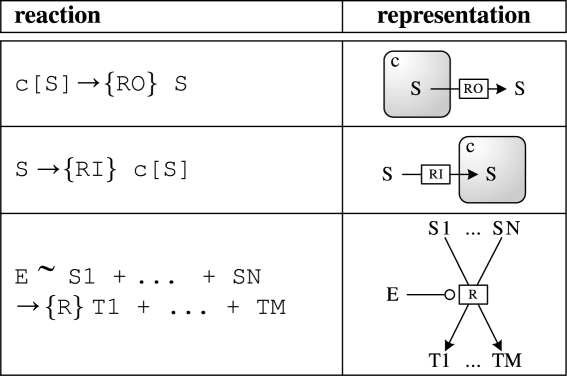
Table 4.

Part properties and their reactions in GEC with their corresponding graphical representation. (Some of the species used in the reactions will also depend on the properties of neighbouring parts.)

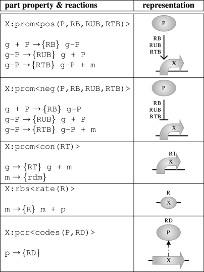The pos and neg properties of promoters each give rise to three reactions: binding and unbinding of the transcription factor and production of mRNA in the bound state. The con property of a promoter yields a reaction producing mRNA in the unbound state, while the rate property of a ribosome binding site yields a reaction producing protein from mRNA. Finally, the codes property of a protein coding region gives rise to a protein degradation reaction. We observe that mRNA degradation rates do not associate naturally with any of the part types since mRNA can be polycistronic in general. Therefore, the rate rdm used for mRNA degradation is assumed to be defined globally, but may be adjusted manually for individual cases where appropriate. Also note that quantities such as protein degradation rates could in principle be stored in the reaction database as degradation reactions. We choose however to keep as much quantitative information as possible about a given part within the parts database.

A part may generally have any number of properties, e.g. indicating the regulation of a promoter by different transcription factors. However, we stress that the abstract language presented in this paper is independent of any particular choice of properties and part types, and that the particular quantitative characterization given in this paper has been chosen for the sake of simplicity. As for the reaction database, we stress that hypothetical rates have been given. Sometimes we may wish to ignore these rates, in which case we assume derived, non-quantitative versions of the properties: for all properties pos(P,RB,RUB,RTB) and neg(P,RB,RUB,RTB), there are derived properties pos(P) and neg(P); and for every property codes(P, RD), there is a derived property codes(P). These derived properties are used in the remainder of the paper. Their corresponding graphical representation is the same as in table 4, but with the rate constants omitted.

The current MIT registry allows parts to be grouped into categories and given unique identifiers, but does not currently make use of a database of possible reactions between parts, nor does it contain a logical characterization of part properties. As such, our overall approach can be used as the basis for a possible extension to the MIT registry, or indeed for the creation of new registries.

2.2. The basics of GEC

2.2.1. Part types

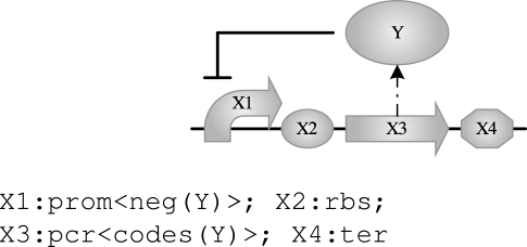
On the most basic level, a program can simply be a sequence of part identifiers together with their types, essentially corresponding to a program in the GenoCAD language. The following program is an example of a transcription unit that expresses the protein tetR in a negative feedback loop, where a corresponding graphical representation is shown above the program code:

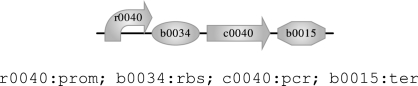The symbol : is used to write the type of a part, and the symbol ; is the sequential composition operator used to put parts together in sequence. Writing this simple program requires the programmer to know that the protein coding region part c0040 codes for the protein tetR and that the promoter part r0040 is negatively regulated by this protein, two facts that we can confirm by inspecting table 1. In this case, the compiler has an easy job: it just produces a single list consisting of the given sequence of part identifiers, while ignoring the types:

2.2.2. Part variables and properties

We can increase the level of abstraction of the program by using variables and properties for expressing that any parts will do, as long as the protein coding region codes for the protein tetR and the promoter is negatively regulated by tetR:

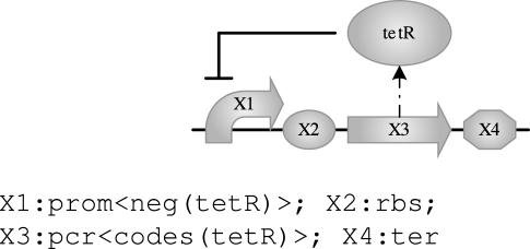The angle brackets <> delimit one or more properties and upper-case identifiers such as X1 represent variables (undetermined part names or species). Compiling this program produces exactly the same result as before, only this time the compiler does the work of finding the specific parts required based on the information stored in the parts database. The compiler may in general produce several results. For example, we can replace the fixed species name tetR with a new variable, thus resulting in a program expressing any transcription unit behaving as a negative feedback device:

This time the compiler produces four devices, one of them being the tetR device from above. When variables are used only once, as is the case for X1, X2, X3 and X4 above, their names are of no significance and we will use the wild card _ instead. When there is no risk of ambiguity, we may omit the wild card altogether and write the above program more concisely as follows:

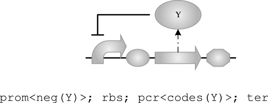2.2.3. Parametrized modules

Parametrized modules are used to add a further level of abstraction to the language. Modules that act as positive or negative gates, or which constitutively express a protein, can be written as follows, where i denotes input and o denotes output:

• module tl(o) {

    rbs; pcr<codes(o)>; ter

  };

• module gatePos(i, o) {

    prom<pos(i)>; tl(o)

  };

• module gateNeg(i, o) {

    prom<neg(i)>; tl(o)

  };

• module gateCon(o) {

    r0051:prom; tl(o)

  };

The module keyword is followed by the name of the module, a list of formal parameters and the body of the module enclosed in brackets {}. For the constitutive expression module, we arbitrarily fix a promoter. Modules can be invoked simply by naming them together with a list of actual parameters, as in the case of the tl module above. These gate modules allow subsequent examples to abstract away from the level of individual parts. The remaining examples in this paper will also use dual-output counterparts of some of these modules, for producing two proteins rather than one:

• module tl2(o1, o2) {

  • rbs; pcr<codes(o1)>;
  • rbs; pcr<codes(o2)>; ter

• };

• module gateCon2(o1, o2) {

  • r0051:prom; tl2(o1, o2)

• };

Note that these modules result in devices that express polycistronic mRNA. A corresponding graphical representation can also be defined for modules, but we omit the details here. For the remaining examples in the paper, the graphical representation will therefore be obtained by expanding the module definitions and by appropriately substituting module bodies for module invocations.

2.2.4. Compartments and reactions

The GEC language also allows the use of compartments which represent the location of the parts, such as a particular cell type. In addition, the language allows reactions to be represented as additional constraints on parts. Table 5 summarizes the reactions available in the language, together with their corresponding graphical representation. The formal syntax and semantics of the GEC language are presented in more detail in §3.

Table 5.

Reactions in the GEC language with their corresponding graphical representation.

2.3. Case study: the repressilator

Our first case study considers the repressilator circuit of Elowitz & Leibler (2000), which consists of three genes negatively regulating each other. The first gene in the circuit expresses some protein A, which represses the second gene; the second gene expresses some protein B, which represses the third gene; and the third gene expresses some protein C, which represses the first gene, thus closing the feedback loop. Using our standard gate modules, the repressilator can be written in GEC as follows:

The expanded form of this program is shown in figure 2, together with the corresponding graphical representation. Compiling the repressilator program produces 24 possible devices. One of these is the following:

Figure 2.

The expanded repressilator program and its corresponding graphical representation.

To see why 24 devices have been generated, an inspection of the databases reveals that there are four promoter/repressor pairs that can be used in the translation of the program: r0011/c0012, r0040/c0040, r0051/c0051 and i0500/c0080. It follows that there are four choices for the first promoter in the target device, three choices for the second promoter and two remaining choices for the third promoter. There is only one ribosome binding site and one terminator registered in the parts database, and hence there are indeed 4.3.2=24 possible target devices.

Our above reasoning reflects an important assumption about the semantics of the language: distinct variables must take distinct values. If we allowed, for example, A and B to represent the same protein, we would get self-inhibiting gates as part of a device and these would certainly prevent the desired behaviour. This assumption seems to be justified in most cases, although it is easy to change the semantics of the language and compiler on a per-application basis, to allow variables to take identical values. We also note that variables range over atomic species rather than complexes, so any promoters that are regulated by dimmers, for example, would not be chosen when compiling the repressilator program.

In the face of multiple possible devices, the question of which device to choose naturally arises. This is where simulation and model refinement become relevant. Figure 3a shows the result of simulating the reactions associated with the above device, which can be found in the electronic supplementary material. We observe that the expected oscillations are not obtained. By further inspection, we discover the failure to be caused by a very low rate of transcription factor unbinding for the promoter i0500: once a transcription factor (araC) is bound, the promoter is likely to remain repressed.

Figure 3.

Stochastic simulation plots of two repressilator devices. (a) The device using clR (red solid lines), tetR (blue dashed lines) and araC (green dotted lines) is defective due to the low rate of unbinding between araC and its promoter, while (b) the device using clR (red solid lines), tetR (blue dashed lines) and lacI (green dotted lines) behaves as expected.

Appropriate ranges for quantitative parameters in which oscillations do occur can be found through further simulations or parameter scans as in Blossey et al. (2008). We can then refine the repressilator program by imposing these ranges as quantitative constraints. This can be done by redefining the negative gate module as follows, leaving the body of the repressilator unmodified:

• module gateNeg(i, o) {

  • new RB. new RUB. new RTB.
  • new RT. new R. new RD.
  • prom<con(RT), neg(i, RB, RUB, RTB)>;
  • rbs<rate(R)>;
  • pcr<codes(o,RD)>; ter |
  • 0.9<RB | RB<1.1 |
  • 0.4<RUB | RUB<0.6 |
  • 0.05<RT | RT<0.15 |
  • RTB<0.01 |
  • 0.05<R | R<0.15

• };

The first two lines use the new operator to ensure that variables are globally fresh. This means that variables of the same name, but under different scopes of the new operator, are considered semantically distinct. This is important in the repressilator example because the gateNeg module is instantiated three times, and we do not necessarily require that the binding rate RB is the same for all three instances. A sequence of part types with properties then follows, this time with rates given by variables, as shown in figure 4. Finally, constraints on these rate variables are composed using the constraint composition operator |. With this module replacing the non-quantitative gate module defined previously, compilation of the repressilator now results in the six devices without the promoter araC, rather than the 24 from before. One of these is the repressilator device contained in the MIT parts database under the identifier I5610:

Figure 4.

The expanded quantitative repressilator program (with quantitative constraints omitted) and the corresponding graphical representation. The quantitative constraints given in the main text restrict rates to a given range, placing further constraints on the parts that can be chosen from the database.

Simulation of the associated reactions now yields the expected oscillations, as shown in figure 3b. Observe also how modularity allows localized parts of a program to be refined without rewriting the entire program.

2.4. Case study: the predator–prey system

Our second case study, an Escherichia coli predator–prey system (Balagaddé et al. 2008) shown in figure 5, represents one of the largest synthetic systems implemented to date. It is based on two quorum-sensing systems, one enabling predator cells to induce expression of a death gene in the prey cells, and the other enabling prey cells to inhibit expression of a death gene in the predator. In the predator, Q1a is constitutively expressed and synthesizes H1, which diffuses to the prey where it dimerizes with the constitutively expressed Q1b. This dimer in turn induces expression of the death protein ccdB. Symmetrically, the prey constitutively expresses Q2a for synthesizing H2, which diffuses to the predator where it dimerizes with the constitutively expressed Q2b. Instead of inducing cell death, this dimer induces expression of an antidote A, which interferes with the constitutively expressed death protein.

Figure 5.

The expanded predator–prey program and the corresponding graphical representation. The simulation-only reactions described in the main text are not represented.

Note how we have left the details of the quorum-sensing system and antidote unspecified by using variables (upper case names) for the species involved. Only the death protein is specified explicitly (using a lower case name). A GEC program implementing the logic of figure 5 can be written as follows:

• module predator() {

  • gateCon2(Q2b, Q1a) |
  • Q1a^∼→H1;
  • Q2b+H2↔Q2b−H2 |
  • gatePos(Q2b−H2, A);
  • gateCon(ccdB) |
  • A ^∼ccdB→|
  • ccdB ^∼ Q1a *→{10.0} |
  • H1 *→{10.0} | H2 *→{10.0}

• };

• module prey() {

  • gatePos(H1−Q1b, ccdB) |
  • H1+Q1b↔H1−Q1b;
  • Q2a^∼→H2 |
  • gateCon2(Q2a, Q1b) |
  • ccdB^∼Q2a *→{10.0} |
  • H1 *→{10.0} | H2 *→{10.0}

• };

• module transport() {

  • c1[H1]→H1 | H1→c2[H1] |
  • c2[H2]→H2 | H2→c1[H2]

• };

• c1[predator()]‖c2[prey()] ‖ transport()

The predator and prey are programmed in two separate modules that reflect our informal description of the system, and a third module links the predator and prey by defining transport reactions. Several additional language constructs are exhibited by this program. Reactions are composed with each other and with the standard gate modules through the constraint composition operator, which is also used for quantitative constraints. Reactions have no effect on the geometrical structure of the compiled program since they do not add any parts to the system, but they restrict the possible choices of proteins and hence of parts. Reversible reactions are an abbreviation for the composition of two reactions. For example, Q2b+H2↔Q2b−H2 is an abbreviation for Q2b+H2→Q2b−H2 | Q2b−H2→Q2b+H2. The last two lines of the predator and prey modules specify reactions that are used for simulation only and do not impose any constraints, indicated by the star preceding the reaction arrows. The second to last line is a simple approach to modelling cell death, and we return to this when discussing simulations shortly. The last line consists of degradation reactions for H1 and H2; since these are not the result of gene expression, the associated degradation reactions are not deduced automatically by the compiler.

The transport module defines transport reactions in and out of two compartments, c1 and c2, representing, respectively, the predator and prey cell boundaries. The choice of compartment names is not important for compilation to parts, but it is important in simulations where a distinction must be made between the populations of the same species in different compartments.

The main body of the program invokes the three modules, while putting the predator and prey inside their respective compartments using the compartment operator. The modules are composed using the parallel composition operator. In contrast to the sequential composition operator which intuitively concatenates the part sequences of its operands, the parallel composition intuitively results in the union of the part sequences of its operands. This is useful when devices are implemented on different plasmids, or even in different cells as in this example. The expanded predator–prey program is shown in figure 5.

Compiling the program results in four devices, each consisting of two lists of parts that implement the predator and prey, respectively. One device is shown below.

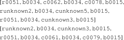By inspection of the database, we establish that the compiler has found luxR/lasI/m3OC12HSL and lasR/luxI/m3OC6HSL for implementing the quorum-sensing components in the respective cells and ccdA2 for the antidote, and that it has found a unique promoter runknown2, which is used both for regulating expression of ccdA2 in the predator and for regulating expression of ccdB in the prey. The fact that the two instances of this one promoter are located in different compartments now plays a crucial role: without the compartment boundaries, undesired crosstalk would arise between lasR-m3OC12HSL and the promoter runknown2 in the predator, and between luxR-m3OC6HSL and the promoter runknown2 in the prey. Indeed, if we remove the compartments from the program, the compiler will detect this crosstalk and report that no devices could be found. This illustrates another important assumption about the semantics of the language: a part may be used only if its ‘implicit’ properties do not contain species which are present in the same compartment as the part. By implicit properties, we mean the properties of a part that are not explicitly specified in the program. In our example, the part runknown2 in the predator has the implicit property that it is positively regulated by lasR-m3OC12HSL. Hence the part may not be used in a compartment in which lasR-m3OC12HSL is present. The use of compartments in our example ensures that this condition of crosstalk avoidance is met.

The reactions associated with the above device are shown in the electronic supplementary material. Simulation results, in which the populations of the killer protein ccdB in the predator and prey are plotted, are shown in figure 6a. We observe that the killer protein in the predator remains expressed, hence blocking the synthesis of H1 through the simulation-only reaction, and preventing expression of killer protein in the prey. This constant level of killer protein in the predator is explained by the low rate at which the antidote protein ccdA2 used in this particular device degrades ccdB, and by the high degradation rate of ccdA2. The second of the four devices is identical to the device above, except that the more effective antidote ccdA is expressed using cunknown4 instead of cunknown5:

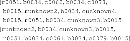Figure 6.

Stochastic simulation plots of two predator–prey devices. (a) The device using ccdA2 is defective due to the low rate of ccdA2-catalysed ccdB degradation, while (b) the device using ccdA behaves as expected (red solid lines, c1[ccdB]; blue dashed lines, c2[ccdB]).

The simulation results of the reactions associated with this device are shown in figure 6b. The two remaining devices are symmetric to the ones shown above in the sense that the same two quorum-sensing systems are used, but they are swapped around such that the predator produces m3OC6HSL rather than m3OC12HSL, and vice versa for the prey.

We stress that the simulation results obtained for the predator–prey system do not reproduce the published results. One reason is that we are plotting the levels of killer proteins in a single predator and a single prey cell rather than cell populations, in order to simplify the simulations. Another reason is that the published results are based on a reduced ordinary differential equation model, and the parameters for the full model are not readily available. Our simplified model is nevertheless sufficient to illustrate the approach, and can be further refined to include additional details of the experimental set-up. We note a number of additional simplifying omissions in our model: expression of the quorum-sensing proteins in the prey, and of the killer protein in the predator, are IPTG induced in the original model; activated luxR (i.e. in complex with m3OC6HSL) dimerizes before acting as a transcription factor; and the antidote mechanism is more complicated than mere degradation (Afif et al. 2001).

3. Methods

In this section, we give a formal definition of GEC in terms of its syntax and semantics. The definition is largely independent of the concrete choice of part types and properties, except for the translation to reactions, which relies on the part types and properties described in the previous section. Here, we focus on the translation to parts, which we consider to be the main novelty, and the translation to reactions is defined formally in the electronic supplementary material.

3.1. The syntax of GEC

3.1.1. The abstract syntax of GEC

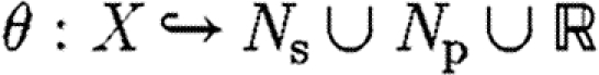
We assume fixed sets of primitive species names N_s, part identifiers N_p and variables X. We assume that x∈X represents variables, n∈N_p represents part identifiers and u∈U represents species, parts and variables, where 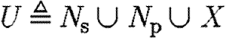. A type system would be needed to ensure the proper, context-dependent use of u, but this is a standard technical issue that we omit here. The set of complex species is given by the set of multisets over N_s∪X and is ranged over by S; multisets (i.e. sets that may contain multiple copies of each element) are used in order to allow for homomultimers.

A fixed set T of part types t is also assumed together with a set ^t of possible part properties for each type t∈T. We define and let range over finite sets of properties of type t. In the case studies, properties are terms over where is the set of real numbers, but the specific structure of properties is not important from a language perspective; all we require is that functions 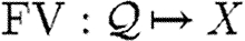and 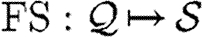are given for obtaining the variables and species of properties, respectively, and we assume these functions to be extended to other program constructs in the standard way.

Finally, c ranges over a given set of compartments, p ranges over a given set of program (module) identifiers, m ranges over the natural numbers , r ranges over and ⊗ ranges over an appropriate set of arithmetic operators. The abstract syntax of GEC is then given by the grammar in table 6. The tilde symbol in the grammar is used to denote lists, and the sum (∑) formally represents multisets.

Table 6.

The abstract syntax of GEC, in terms of programs P, constraints C and reactions R, where the symbol ⋮ is used to denote alternatives. (Programs consist of part sequences, modules, compartments and constraints, together with localized variables. The definition is recursive, in that a large program can be made up of smaller programs. Constraints consist of reactions and parameter ranges.)

P::=u:t(Qt)	part u of type t with properties Qt
⋮0	empty program
	definition of module p with formals
	invocation of module p with actuals
⋮P|C	constraint C associated to program P
⋮ P1∥P2	parallel composition of P1 and P2
⋮ P1; P2	sequential composition of P1 and P2
⋮ c[P]	compartment c containing program P
⋮ new x.P	local variable x inside program P
C::=R	reaction
⋮ T	transport reaction
⋮ K	numerical constraint
⋮ C1|C2	conjunction of C1 and C2
	reactants Si, products Sj
T::=S→rc[S]	transport of S into compartment c
⋮ c[S]→rS	transport of S out of compartment c
K::=E1>E2	expression E1 greater than E2
E::=r	real number or variable
⋮ E1⊗E2	arithmetic operation ⊗ on E1 and E2
A::=r	real number or variable
⋮ S	species

3.1.2. Derived forms

Some language constructs are not represented explicitly in the grammar of table 6, but can easily be defined in terms of the basic abstract syntax. Reversible reactions are defined as the parallel composition of two reactions, each representing one of the directions. We use the underscore (_) as a wild card to mean that any name can be used in its place. This wild card can be encoded using variables and the new operator; for example, we define . In the specific case of basic part programs, we will often omit the wild card, i.e. . We also allow constraints to be composed to the left of programs and define .

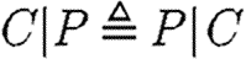3.1.3. The concrete syntax of GEC

The examples of GEC programs given in this paper are written in a concrete syntax understood by the implemented parser. The main difference compared to the abstract syntax is that variables are represented by upper case identifiers and names are represented by lower case identifiers. Complex species are represented by lists separated by the (−) symbol in the concrete syntax, and the fact that complex species are multisets in the abstract syntax reflects that this operator is commutative (i.e. ordering is not significant). Similar considerations apply to the sum operator in reactions. We also assume some standard precedence rules, in particular that (;) binds tighter than (‖), and allow the use of parentheses to override these standard rules if necessary.

3.2. The semantics of GEC

We first illustrate the semantics of GEC informally through a small example, which exhibits characteristics from the predator–prey case study, and then turn to the formal presentation.

3.2.1. A small example

The translation uses the notion of context-sensitive substitutions (θ,ρ,σ,τ) to represent solutions to the constraints of a program, where θ is a mapping from variable names to primitive species names, part names or numbers; ρ is a set of variables that must remain distinct after the mapping is applied; σ and τ are, respectively, the species names that have been used in the current context and the species names that are excluded for use. This information is necessary in order to ensure piecewise injectivity over compartment boundaries, together with crosstalk avoidance, as mentioned in the case studies. The translation also uses the notion of device templates. These are sets containing lists over part names and variables, and a context-sensitive substitution can be applied to a device template in order to obtain a final concrete device. Consider the following example:

The translation first processes the two sequential compositions in isolation, and then the parallel composition.

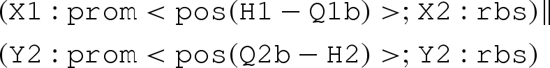
1. Observe that the database only lists a single promoter part that is positively regulated by a dimer, namely runknown2. The first sequential composition gives rise to the device template {[X1,X2]} and two context-sensitive substitutions, one for each possible choice of transcription factors listed in the database for this promoter part. These are (θ₁,ρ₁,σ₁,τ₁) and where

   • —θ₁={(X1↦runknown2),(X2↦b0034), (H1↦m3OC12HSL),(Q1b↦lasR)}.
   • —ρ₁={H1,Q1b}.
   • —σ₁={m3OC12HSL−lasR}.
   • —τ₁={m3OC6HSL−luxR}.
   • —={(X1↦runknown2),(X2↦b0034), (H1↦m3OC6HSL),(Q1b↦luxR)}.
   • —={H1,Q1b}.
   • —={m3OC6HSL−luxR}.
   • —={m3OC12HSL−lasR}.

   Note that τ₁={m3OC6HSL−luxR}, since the complex m3OC6HSL−luxR is in the properties of runknown2, but has not been mentioned explicitly in the program under the corresponding substitution θ₁. Therefore, this complex should not be used anywhere in the same compartment as runknown2, in order to prevent unwanted interference between parts. Similar ideas apply to .

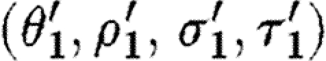
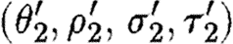
2. The second sequential composition produces equivalent results, namely the device template {[Y1,Y2]} and two context-sensitive substitutions, one for each possible choice of transcription factors in the database for the promoter part. These are (θ₂,ρ₂,σ₂,τ₂) and where

   • —θ₂={(Y1↦runknown2),(Y2↦b0034), (H2↦m3OC12HSL),(Q2b↦lasR)}.
   • —ρ₂={H2,Q2b}.
   • —σ₂={m3OC12HSL−lasR}.
   • —τ₂={m3OC6HSL−luxR}.
   • —={(Y1↦runknown2),(Y2↦b0034), (H2↦m3OC6HSL),(Q2b↦luxR)}.
   • —={H2,Q2b}.
   • —={m3OC6HSL−luxR}.
   • —={m3OC12HSL−lasR}.

3. The parallel composition can now be evaluated by taking the union of device templates from the two components, resulting in {[X1,X2],[Y1,Y2]}. However, none of the context-sensitive substitutions are compatible. We can combine neither θ₁ and θ₂, nor and , because the union of these is not injective on the corresponding domains determined by ρ₁∪ρ₂ and , respectively. And we can combine neither θ₁ and , nor and θ₂, because the corresponding used species and exclusive species overlap. This can be overcome by placing each parallel component inside a compartment as in the predator–prey case study. The compartment operator simply disregards the injective domain variables, the used names and the exclusive names of its operands, after which all the four combinations of substitutions mentioned above would be valid. In this example, all four resulting substitutions map the part variables to the same part names, and hence only the single device {[runknown2,b0034],[runknown2,b0034]} results.

3.2.2. Formal definition

Transport reactions contain explicit compartment names that are important for simulation, but only the logical property that transport is possible is captured in the parts database. We therefore define the operator (.)^↓ on transport reactions to ignore compartment names, where 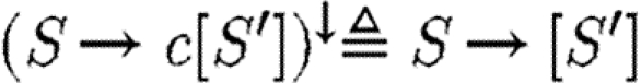and 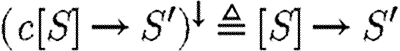. The meaning of a program is then given relative to global databases _b and _r of parts and reactions, respectively. For the formal treatment, we assume these to be given by two finite sets of ground terms:

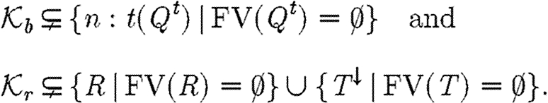In the following, we use Dom(θ) and Im(θ) to denote, respectively, the domain and image of a function θ. We then define CS to be the set of context-sensitive substitutions (θ,ρ,σ,τ), where

1. is a finite, partial function (the substitution).

2. ρ⫋X is a set of variables over which θ is injective, i.e. .

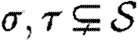3. are, respectively, the species names that have been used in the current context and the species names that are excluded for use, and σ∩τ=.

Context-sensitive substitutions represent solutions to constraints. They also capture the information necessary to ensure piecewise injectivity over compartment boundaries, together with crosstalk avoidance, as mentioned in the case studies and in the earlier example. We define the composition of two sets of context-sensitive substitutions as follows:

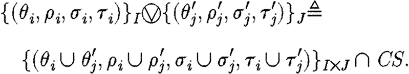Informally, the composition consists of all possible pairwise unions of the operands that satisfy the conditions of context-sensitive substitutions. This means in particular that the resulting substitutions are indeed functions, they are injective over the relevant interval and they originate from pairs of context-sensitive substitutions, for which the used names in one are disjoint from the excluded names in the other. So in practice, if two sets of context-sensitive substitutions represent the solutions to the constraints of two programs, their composition represents the solutions to the constraints of the composite program (e.g. the parallel or sequential compositions). From now on, we omit the indices I and J from indexed sets when they are understood from the context.

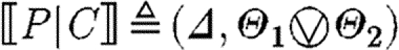
The target semantic objects of the translation we wish to define on programs are pairs (Δ,Θ) of device templates Δ⫋U^*, i.e. sets of lists over variables and names, and sets Θ⫋CS of context-sensitive substitutions. The intuition is that each context-sensitive substitution in Θ satisfies the constraints given implicitly by a program, and can be applied to the device template to obtain the final, concrete device. We write Dom_s(θ) for the subset of the domain of θ mapping to species names, i.e. 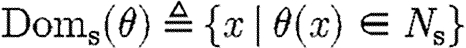, and we write Im_s(θ) for the species names in the image of θ, i.e. 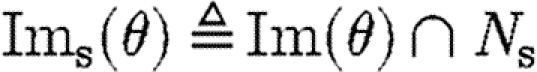. The denotational semantics of GEC is then given by a partial function of the form 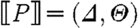, which maps a program P to a set Δ of device templates and a set Θ of substitutions. It is defined inductively on programs with selected cases shown below; the full definition, which includes a treatment of modules and module environments, is given in the electronic supplementary material.

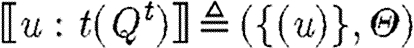1. , where

   

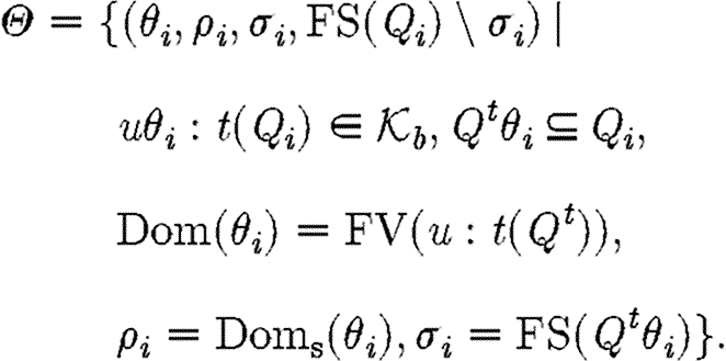
2. , where

   

3. , where

   

4. , where

   

5. ,where

   

6. .

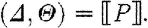
In the first case, the denotational function results in a single sequence consisting of one part. The associated substitutions represent the possible solutions to the constraint that the part with the given properties must be in the database. The substitutions are required to be defined exactly on the variables mentioned in the program and to be injective over these. The excluded names are those which are associated with the part in the database, but not stated explicitly in the program.

The case (ii) for a program with constraints produces the part sequences associated with the semantics for the program, since the constraints do not give rise to any parts; the resulting substitutions arise from the composition of the substitutions for the program and for the constraints. The case (iii) for parallel composition produces all the part sequences resulting from the first component together with all the part sequences resulting from the second component, i.e. the union of two sets, and the usual composition of substitutions. The case (iv) for sequential composition differs only in the Cartesian product of part sequences instead of the union, i.e. we get all the sequences resulting from concatenating any sequence from the first program with any sequence from the second program.

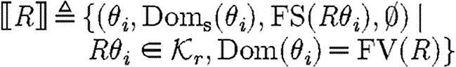
The case (v) for compartments simply produces the part sequences from the contained program together with the substitutions, except that it ‘forgets’ about the injective domain, used names and restricted names. Hence subsequent compositions of the compartment program with other programs will not be restricted in the use of names, reflecting the intuition that crosstalk is not a concern across compartment boundaries, as illustrated in the predator–prey case study. The last case for reactions follows the same idea as the first case for parts, except that the reaction database is used instead of the parts database. Observe finally that the semantics is compositional in the sense that the meaning of a composite program is defined in terms of the meaning of its components.

3.2.3. Properties of the semantics

Recall the requirements for the translation alluded to in the case studies. The first requirement is piecewise injectivity of substitutions over compartments: distinct species variables within the same compartment must take distinct values. The second requirement is non-interference: a part may be used only if its implicit properties do not contain species that are present in the same compartment as the part. These requirements are formalized in propositions 3.1 and 3.2. We use contexts (⋅) to denote any program with a hole, and (P) to denote the context with the (capture-free) substitution of the hole for P. The free program identifiers of P, defined in a standard manner with program definitions as binding constructs, are denoted by FP(P).

Proposition 3.1 (piecewise injectivity)

For any context and any compartment-free program P with FP(P)=, , it holds that θ_i is injective on the domain FV(P)∩Dom_s(θ_i).

Proposition 3.2 (non-interference)

For any basic program and any compartment-free context with , it holds that for some Q and .

Proofs are by induction and can be found in the electronic supplementary material.

3.3. Implementation

A parser for recognizing the syntax of GEC programs has been implemented using the parser generator tools of the F# programming language. A corresponding translator, also implemented in F#, conceptually follows the given denotational semantics (Pedersen & Phillips 2009). The translator generates constraints rather than substitutions and subsequently invokes the ECLiPSe Prolog engine (Apt & Wallace 2007) for solving these constraints. We have presented the denotational semantics in terms of substitutions for the sake of clarity, but the corresponding constraints are implicit and can be extracted by inspection. The translator also generates reactions by directly taking the reactions contained in programs after substituting formal for actual parameters, and by extracting reactions from the relevant parts as indicated earlier.

4. Discussion

The databases used for the case studies have been created with the minimal amount of information necessary to convey the main ideas of our approach. An immediate obstacle therefore arises in the practical application of GEC to novel problems: the databases needed for translation of general programs do not yet exist, partly because the necessary information has not yet been formalized on a large scale. In spite of this, we believe that GEC does contribute important steps towards the ultimate dream of compilable high-level languages for synthetic biology. In the following, we outline these contributions and proceed to discuss future directions for developing the language.

4.1. Contributions

To our knowledge, GEC is the first formal language that allows synthetic systems to be described at the logical level of interactions between potentially undetermined proteins and genes, while affording a translation to sequences of genetic parts and to reactions. As such, it provides a concrete basis for discussing the design of future languages for synthetic biology. In particular, we have introduced the elementary notions of parts with properties and constraints, and a set of operators with natural interpretations in the context of synthetic biology. We have also shown how parametrized modules can be used to abstract away from the layer of parts, and how modules in general can be used to program systems in a structured manner. The question of whether distinct variables should be allowed to take identical values has been raised, and we have shown how undesired crosstalk between parts in the same compartment can be detected and avoided by the compiler. These concepts have been defined formally and validated in practice through case studies and the implementation of a compiler.

The parts database, in spite of being incomplete, points towards the logical properties that must be formally associated with parts if languages and compilers of the kind presented in this paper are to be used in practice. For example, promoters should be associated with details of positive and negative regulation, and protein coding regions should be associated with a unique identifier of the protein they code for. These observations may contribute to the efforts of part standardization, which so far seem to have focused on biological, rather than logical, properties of parts.

An important benefit of representing systems in a formal language is that their meaning is precisely and unambiguously defined. This benefit also applies to synthetic biology, where informal diagrams of protein and gene networks are often difficult for outsiders to interpret. In this respect, GEC can be used as a formal representation of novel systems, and databases can be constructed on a per-application or per-organism basis, thus serving to formally capture the assumptions of a given project. Furthermore, the notion of a reaction database, which is perhaps the largest practical hurdle, can be completely omitted by prefixing reaction arrows with a star (*) in programs, effectively tagging them as simulation only in which case they will not be used in constraint generation. Such an approach may be relevant in educational contexts, e.g. the International Genetically Engineered Machine competition, where students may benefit from gaining an understanding of formal languages.

4.2. Challenges and future directions

The reaction database has been designed with simplicity in mind, by recording potential enzymes, reactants and products for each reaction. The transport reactions also capture notions of compartment boundaries. But reactions may generally be represented on multiple levels of detail, such as the lower level of binding domains and modification sites that is common when modelling signalling pathways. This in turn could tie in with the use of protein domain part types, which are already present to some extent in the Registry of Standard Biological Parts. An important and non-trivial future challenge is therefore to address this question of representation.

For any given representation, however, logic programming can be used to design further levels of deductive reasoning. A simple example would be the notion of indirect regulation, such as a promoter that is indirectly positively regulated by s, which would have the property ipos(s), if either (i) it has the property pos(s) or (ii) it has the property neg(s′) and there is a reaction s+s′→s−s′. A deductive approach to the analysis of genes, implemented using theorem proving in the tool BioDeductiva, is discussed in Shrager et al. (2007). This approach is likely to also work with biochemical reactions, in which case linking the compiler to this tool may be of interest. However, the challenge of formalizing the data representation and deductive layers in this framework remains.

With additional deductive power also comes increased computational complexity. Our current Prolog-based approach is unlikely to scale with increasing numbers of variables in programs, partly because the search for solutions is exhaustive and unguided, and also because the order in which constraints are tested is arbitrarily chosen as the order in which they occur in the GEC programs. Future work should seek to ameliorate these problems through the use of dedicated constraint logic-programming techniques, which we anticipate can be added as extensions to our current approach by using the facilities of the ECLiPSe environment.

More work is also needed to increase the likelihood that devices generated by the compiler do in fact work in practice, for example by taking into account compatibility between parts and compatibility with target cells. Quantitative constraints are another important means to this end, and we have indicated how mass action rate constants can be added to parts. While such a representation is simple, it does not account for the notion of fluxes, measured for example in polymerases per second or ribosomes per second and used for instance in Marchisio & Stelling (2008). But imposing meaningful constraints on fluxes, which are expressed as first-order derivatives of real functions, is not an easy task and remains an important future challenge. The related issue of accommodating cooperatively regulated promoters, such as those described in Buchler et al. (2003), Hermsen et al. (2006) and Cox et al. (2007), also remains to be addressed.

Another issue that needs to be considered is the potential impact of circuits on the host physiology, such as the metabolic burden that can be caused by circuit activation. This is an important issue in the design of synthetic gene circuits, as discussed for example in Andrianantoandro et al. (2006) and Marguet et al. (2007). One way to account for this impact is to include an explicit model of host physiology when generating the reactions of a given GEC program for simulation. For instance, the degradation machinery of a host cell could be modelled as a finite species, and protein degradation could be modelled as an interaction with this species, rather than as a simple delay. As the number of proteins increases, the degradation machinery would then become overloaded and the effects would be observed in the simulations. More refined models of host physiology could also be included by refining the corresponding part properties accordingly.

On a practical note, much can be done to improve the prototype implementation of the compiler, including for example better support for error reporting. Indeed, it is possible to write syntactically well-formed programs that are not semantically meaningful, e.g. by using a complex species where a part identifier is expected. Such errors should be handled through a type system, but this is a standard idea which has therefore not been the focus of the present work. Neither have the efforts of the GenoCAD tool been duplicated, so the compiler will not refuse programs that do not adhere to the structure set forth by the GenoCAD language. We do, however, show in the electronic supplementary material how the GenoCAD language can be integrated into our framework in a compositional manner. Finally, practical applications will require extensions of the current minimal databases, which may lead to additional part types or properties.

References

- Afif H., Allali N., Couturier M., Van Melderen L. 2001. The ratio between ccda and ccdb modulates the transcriptional repression of the ccd poison-antidote system. Mol. Microbiol. 41, 73–82. ( 10.1046/j.1365-2958.2001.02492.x) [DOI] [PubMed] [Google Scholar]
- Andrianantoandro E., Basu S., Karig D., Weiss R. 2006. Synthetic biology: new engineering rules for an emerging discipline. Mol. Syst. Biol. 2, 2006.0028 ( 10.1038/msb4100073) [DOI] [PMC free article] [PubMed] [Google Scholar]
- Apt K. R., Wallace M. G. 2007. Constraint logic programming using ECLiPSe. Cambridge, UK: Cambridge University Press [Google Scholar]
- Balagaddé F., Song H., Ozaki J., Collins C., Barnet M., Arnold F., Quake S., You L. 2008. A synthetic Escherichia coli predator–prey ecosystem. Mol. Syst. Biol. 4, 187 ( 10.1038/msb.2008.24) [DOI] [PMC free article] [PubMed] [Google Scholar]
- Bergmann F. T., Sauro H. M. 2006. SBW—a modular framework for systems biology. In WSC '06: Proc. 38th Conf. on Winter Simulation, pp. 1637–1645. [Google Scholar]
- Blossey R., Cardelli L., Phillips A. 2008. Compositionality, stochasticity and cooperativity in dynamic models of gene regulation. HFSP J. 2, 17–28. ( 10.2976/1.2804749) [DOI] [PMC free article] [PubMed] [Google Scholar]
- Bornstein B. J., Keating S. M., Jouraku A., Hucka M. 2008. LibSBML: an API library for SBML. Bioinformatics. 24, 880–881. ( 10.1093/bioinformatics/btn051) [DOI] [PMC free article] [PubMed] [Google Scholar]
- Buchler N. E., Gerland U., Hwa T. 2003. On schemes of combinatorial transcription logic. Proc. Natl Acad. Sci. USA. 100, 5136–5141. ( 10.1073/pnas.0930314100) [DOI] [PMC free article] [PubMed] [Google Scholar]
- Cai Y., Hartnett B., Gustafsson C., Peccoud J. 2007. A syntactic model to design and verify synthetic genetic constructs derived from standard biological parts. Bioinformatics. 23, 2760–2767. ( 10.1093/bioinformatics/btm446) [DOI] [PubMed] [Google Scholar]
- Chabrier-Rivier N., Fages F., Soliman S. 2004. The biochemical abstract machine BIOCHAM. In Proc. CMSB, vol. 3082 (eds Danos V., Schächter V.). Lecture Notes in Computer Science, pp. 172–191. Berlin, Germany: Springer. [Google Scholar]
- Ciocchetta F., Hillston J. 2008. Bio-pepa: an extension of the process algebra pepa for biochemical networks. Electron. Notes Theor. Comput. Sci. 194, 103–117. ( 10.1016/j.entcs.2007.12.008) [DOI] [Google Scholar]
- Cox R. S., III, Surette M. G., Elowitz M. B. 2007. Programming gene expression with combinatorial promoters. Mol. Syst. Biol. 3, 145> ( 10.1038/msb4100187) [DOI] [PMC free article] [PubMed] [Google Scholar]
- Danos V., Feret J., Fontana W., Harmer R., Krivine J. 2007. Rule-based modelling of cellular signalling. In CONCUR, vol. 4703 (eds Caires L., Vasconcelos V. T.). Lecture Notes in Computer Science, pp. 17–41. Berlin, Germany: Springer; Tutorial paper. [Google Scholar]
- Elowitz M. B., Leibler S. 2000. A synthetic oscillatory network of transcriptional regulators. Nature. 403, 335–338. ( 10.1038/35002125) [DOI] [PubMed] [Google Scholar]
- Endy D. 2005. Foundations for engineering biology. Nature. 438, 449–453. ( 10.1038/nature04342) [DOI] [PubMed] [Google Scholar]
- Fisher J., Henzinger T. 2007. Executable cell biology. Nat. Biotechnol. 25, 1239–1249. ( 10.1038/nbt1356) [DOI] [PubMed] [Google Scholar]
- Garfinkel D. 1968. A machine-independent language for the simulation of complex chemical and biochemical systems. Comput. Biomed. Res. 2, 31–44. ( 10.1016/0010-4809(68)90006-2) [DOI] [PubMed] [Google Scholar]
- Hermsen R., Tans S., Wolde P. R. 2006. Transcriptional regulation by competing transcription factor modules. PLoS Comput. Biol. 2, 1552–1560. ( 10.1371/journal.pcbi.0020164) [DOI] [PMC free article] [PubMed] [Google Scholar]
- Hucka M., et al. 2003. The systems biology markup language (SBML): a medium for representation and exchange of biochemical network models. Bioinformatics. 19, 524–531. ( 10.1093/bioinformatics/btg015) [DOI] [PubMed] [Google Scholar]
- Mallavarapu A., Thomson M., Ullian B., Gunawardena J. 2009. Programming with models: modularity and abstraction provide powerful capabilities for systems biology. J. R. Soc. Interface. 6, 257–270. ( 10.1098/rsif.2008.0205) [DOI] [PMC free article] [PubMed] [Google Scholar]
- Marchisio M. A., Stelling J. 2008. Computational design of synthetic gene circuits with composable parts. Bioinformatics. 24, 1903–1910. ( 10.1093/bioinformatics/btn330) [DOI] [PubMed] [Google Scholar]
- Marguet P., Balagadde F., Tan C., You L. 2007. Biology by design: reduction and synthesis of cellular components and behaviour. J. R. Soc. Interface. 4, 607–623. ( 10.1098/rsif.2006.0206) [DOI] [PMC free article] [PubMed] [Google Scholar]
- Pedersen M., Phillips A. 2009. GEC tool. See http://research.microsoft.com/gec.
- Pedersen M., Plotkin G. 2008. A language for biochemical systems. In Proc. CMSB (eds Heiner M., Uhrmacher A. M.). Lecture Notes in Computer Science Berlin, Germany: Springer. [Google Scholar]
- Regev A., Silverman W., Shapiro E. 2001. Representation and simulation of biochemical processes using the pi-calculus process algebra. In Pacific Symp. on Biocomputing, pp. 459–470. [DOI] [PubMed] [Google Scholar]
- Sauro H. 2000. Jarnac: a system for interactive metabolic analysis. In Animating the cellular map: Proc. 9th Int. Meeting on BioThermoKinetics (eds Hofmeyr J.-H., Rohwer J., Snoep J.), pp. 221–228. Stellenbosch, Republic of South Africa: Stellenbosch University Press. [Google Scholar]
- Shrager J., Waldinger R., Stickel M., Massar J. 2007. Deductive biocomputing. PLoS ONE. 2, e339 ( 10.1371/journal.pone.0000339) [DOI] [PMC free article] [PubMed] [Google Scholar]