Methods for improving simulations of biological systems: systemic computation and fractal proteins

Abstract

Modelling and simulation are becoming essential for new fields such as synthetic biology. Perhaps the most important aspect of modelling is to follow a clear design methodology that will help to highlight unwanted deficiencies. The use of tools designed to aid the modelling process can be of benefit in many situations. In this paper, the modelling approach called systemic computation (SC) is introduced. SC is an interaction-based language, which enables individual-based expression and modelling of biological systems, and the interactions between them. SC permits a precise description of a hypothetical mechanism to be written using an intuitive graph-based or a calculus-based notation. The same description can then be directly run as a simulation, merging the hypothetical mechanism and the simulation into the same entity. However, even when using well-designed modelling tools to produce good models, the best model is not always the most accurate one. Frequently, computational constraints or lack of data make it infeasible to model an aspect of biology. Simplification may provide one way forward, but with inevitable consequences of decreased accuracy. Instead of attempting to replace an element with a simpler approximation, it is sometimes possible to substitute the element with a different but functionally similar component. In the second part of this paper, this modelling approach is described and its advantages are summarized using an exemplar: the fractal protein model. Finally, the paper ends with a discussion of good biological modelling practice by presenting lessons learned from the use of SC and the fractal protein model.

1. Understanding modelling and simulation

Computer formalisms, simulations and models are becoming increasingly important tools for the natural sciences. In computer science, entire fields now exist that are based purely on the tenets of simulation and modelling of biological processes (e.g. computational neuroscience: Holmes et al. 2008; artificial life: Bullock et al. 2008; computational biology: Wren et al. 2008). In the developing fields of synthetic biology, DNA computing and living technology, computer modelling plays a vital role in the design, testing and evaluation of almost every stage of the research1 (e.g. Blain et al. 2004; Rudge & Haseloff 2005; Dupuy et al. 2007). It is thus perhaps surprising that very little consideration is given to the process of modelling and simulation itself (Webb 2001). Out of necessity, all models must be abstractions from reality. Thus, all models are wrong in some respect by design (or more commonly, by accident). But how should these abstractions be designed? How wrong is your model?

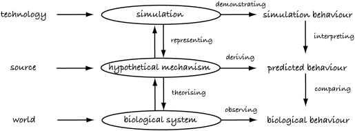
In this paper, we focus on models and simulations that aim to represent and explain the internal workings of a biological system. Figure 1 illustrates a typical view of the simulation process (based on Webb 2001). We typically begin with a biological system under consideration, which exists in the world and has an observable behaviour. Next, some hypothetical mechanism2 is developed from a source, from which a predicted behaviour is hypothesized. In some cases, it may be possible to theorize the hypothetical mechanism directly from the biological system or the biological system from the hypothetical mechanism. Likewise, it may be possible to compare the predicted behaviour with the biological behaviour and refute (or provide supporting evidence for) the hypothetical mechanism and predicted behaviour directly. However, in many cases, this is not possible due to the lack of data or practical constraints in testing. The solution is to use some form of technology to create a simulation or model that represents or encapsulates the hypothetical mechanism, i.e. we produce a simulation of the biological system according to how we think it works. The simulation uses technology to produce some behaviours and enables fast production of data. Significantly for this paper, the quality of the simulation is assessed by comparing how its behaviour matches the predicted behaviour (does it behave in the way we believe the biological system behaves) and how well it represents the hypothetical mechanism (does it model the workings of the biological system in the way we believe the biological system works).

Figure 1.

The simulation process, adapted from fig. 1 of Webb (2001).

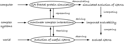
Webb's framework can be illustrated through a simple example (figure 2). The biological system under consideration might be ‘the evolution of protein and gene interactions of eukaryotes’, with the behaviour of interest being ‘how evolution is able to form useful gene regulatory networks’ (GRNs). When attempting to create the hypothetical mechanism, the source might be from a completely different field, for example the mathematics of complex systems. The hypothetical mechanism might then be ‘natural selection of nonlinear interactions with specific properties between proteins and between genes and proteins’, which implies a predicted behaviour that ‘evolution is better able to design useful GRNs given the hypothetical mechanism’. In this example, gathering data on long-term evolutionary trends on GRNs of differing complexities in eukaryotes is not feasible. Thus, we might use a computer to simulate the evolution of GRNs using a genetic algorithm (GA) and model protein shapes using fractals (we return to this example later in the paper).

Figure 2.

Example of an actual simulation design adapted from Webb's (2001) framework.

The justification for simulation is simple. Following Webb's framework again (figure 1), if we propose a mechanism by which we believe a biological system works, and create a simulation which properly represents that mechanism, then comparing (which may require interpretation) predicted behaviour with simulated behaviour can provide evidence that our hypothesis may have some merit. If we also compare the predicted behaviour with actual behaviour of the biological system, we have further evidence that our hypothetical mechanism may be plausible. Chan & Tidwell (1993) concisely summarize this process: we theorize that a system is of type T, and construct an analogous system to T, to see whether it behaves similar to the target system.

But, if we propose a mechanism by which we believe a biological system works, and the simulation misrepresents that mechanism, then no useful evidence can be gained by comparing simulated behaviour with predicted behaviour. Or to use the terminology of Chan & Tidwell (1993): if we theorize that a system is of type T, and construct a system that behaves as we predict T behaves, but is not analogous to T, then we have no useful evidence, despite the apparent matching behaviours.

The same pitfall arises if we construct a hypothetical mechanism that appears to have the same predicted behaviour as the biological system, but the theorizing is flawed. The evidence of matching behaviours is of little help if the biological system actually generates its behaviours through entirely different means to those theorized. (It may look like a duck and quack like a duck—but it may not be a duck at all.)

These pitfalls form the main stumbling blocks of analysis and simulation of biological systems.3 Experience suggests that it is astonishingly common for hypothetical mechanisms and simulations to be created that appear to match biological behaviours and predicted behaviours very well according to numerical analysis. They do so because they have been designed to do so, and not because their internal workings and mechanisms resemble the actual biological system.

Given sufficient experimentation to gather the data of all behaviours (including those not specified in the design of the hypothetical mechanisms and simulations), these pitfalls can in theory be avoided. In practice, time and monetary constraints prevent comprehensive testing, so all comparisons are always performed using partial, incomplete and often very noisy data. Our only recourse in such situations is thus also to examine the process of hypothetical mechanism creation, and simulation creation.

When assessing the quality and validity of a simulation, one established approach is to use formal mathematical methods to prove that the simulation is exactly as defined in the hypothetical mechanism. (For example, pi-calculus and other process algebras enable such proofs (Milner 1993, 2005).) The advantage of the approach is that there can be no doubt that the representation is accurate and correct. The disadvantage is that the hypothetical mechanism and simulation typically become unwieldy, unintuitive and difficult for those unfamiliar with such calculi to interpret. There are also practical limits on the complexity of models that can be simulated in this way.

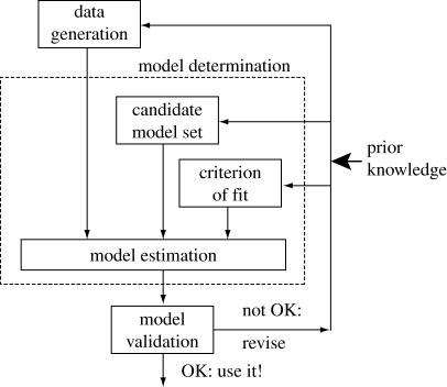
The problem of model creation is hardly new, however. The control systems engineering community is largely responsible for developing and advancing the field of system identification, where the goal is to build models that describe how the behaviour of a system relates to external influences (inputs to the system). Their initial contributions began shortly after the establishment of modern control theory in the 1960s. At present, the field is very mature and several comprehensive textbooks on the subject matter exist (Juang 1993; Nelles 2000). The system identification method is an iterative process consisting of three basic steps: (i) data generation, (ii) model determination, and (iii) model validation (figure 3). Model estimation can be compared with Webb's hypothetical mechanism. If the model is not validated, then steps (i) and/or (ii) are adjusted and the ensuing steps are repeated until successful model validation is achieved. A priori knowledge is injected into this process wherever possible (Xinshu et al. 2005).

Figure 3.

Adapted from the figure of Xinshu et al. (2005).

Many researchers attempt to improve the methodology of modelling, for example the framework of Stepney et al. (2005). But given the difficulties involved, it is perhaps not surprising that the process of modelling and simulation is filled with ambiguity and disagreement. Models are always wrong, but when models are created and techniques applied using questionable methodologies, it is not always clear how they are wrong. Is the hypothetical mechanism incorrect? (i.e. have we misunderstood the biology?) Is the simulation invalid? (i.e. are we truly simulating the hypothetical mechanism or are we just using software to create the results we are hoping to see?)

In an attempt to simplify the many layers of analysis and simulation favoured by some, recent work introduced by the author (Bentley 2007) takes an alternative approach. Instead of using one language and/or representation to define the hypothetical mechanism and another for the simulation, with additional proofs and checking required to prove their equivalence, this work proposes a single biological modelling language to express both. Using this approach, the biological system can be analysed and a hypothetical mechanism developed. The same mechanism can then be run as a simulation, using the simulation behaviour as the predicted behaviour. With this approach, all that remains is theorizing (is the model right?) and comparing (does the model behave correctly?; figure 4).

Figure 4.

Systemic computation (SC) is designed to provide a language with which to describe the hypothetical mechanisms behind biology. SC is also a Turing complete computer, so any model described using SC can be run as a program, turning it into a simulation with its systemic behaviour.

2. Overview of systemic computation

‘Systemics’ is a world view where traditional reductionist approaches are supplemented by holistic, system-level analysis. Instead of relying on a notion of compartmentalizing a natural system into components, analysing each in isolation and then attempting to fit the pieces into a larger jigsaw, a systemic approach would recognize that each component may be intricately entwined with the other components and would attempt to analyse the interplay between components and their environment at many different levels of abstractions (Eriksson 1997). For example, a reductionist analysis of the immune system might reach very specific conclusions about the effect of certain stimuli on certain cells (e.g. freezing of cells in culture, which causes necrosis). A systemic approach might recognize that the real immune system would never encounter such stimuli in isolation (cold temperatures cause many important physiological effects in the body, which would change the environment of the cells), and thus the results may be inaccurate or irrelevant.

‘Systemic computation’ (SC) is a method of computation proposed in Bentley (2007), which uses the systemics world view and incorporates a series of important attributes of natural computation, including: stochasticity, asynchrony, parallelism, homeostasis, open-endedness, distribution, approximate, embodied and circular causality (Bentley 2007). The method builds upon many existing concepts such as object-oriented programming, flow diagrams, graph-based notations and previous models of computation, but is biased towards the representation of natural and biological features. Instead of the traditional centralized view of computation, here all computation is distributed. There is no separation of data and code, or functionality into memory, arithmetic logic unit (ALU) and input/output, as is traditional in contemporary computer architectures. Everything in SC is composed of systems, which may not be destroyed, but may transform each other through their interactions, akin to collision-based computing (Adamatzky 2002). Two systems interact in the context of a third system, which defines the result of their interaction. This is intended to mirror all conceivable natural processes, e.g.

• —molecular interactions (two molecules interact according to their shape, within a specific molecular and physical environment),

• —cellular interactions (intercellular communication and physical forces imposed between two cells occur in the context of a specific cellular environment), and

• —individual interactions (evolution relies on two individuals interacting at the right time and context, both to create offspring and to cause selection pressure through death).

Systems have some form of ‘shape’4 that determines which other systems they can interact with and the nature of that interaction. The shape of a contextual system affects the result of the interaction between systems in its context. Figure 5 illustrates this concept: the resultant transformation of two interacting systems is dependent on the context in which that interaction takes place. A different context will produce a different transformation. Since everything in SC is a system, context must be defined by a system.

Figure 5.

Two systems interacting (colliding, in this example). The systems have properties of size, shape, composition, position and velocity, some or all of which will be transformed as a result of the interaction. The transformation is dependent on the context in which the interaction takes place; here the context includes gravity, friction, elasticity, inertia, temperature and space–time. Within a different context, the interaction will have a different resultant transformation.

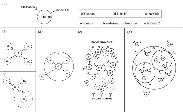
In order to represent these notions computationally, the notions of schemata and transformation functions are used. The shape of a system in this model is the combination of schemata and function, so specific regions of that shape determine the meaning and effect of the system when behaving as a context or interacting. Thus, each system comprises three elements: two schemata that define the possible systems that may interact in the context of the current system5 and the transformation function, which defines how the two interacting systems will be transformed (figure 6a). This behaviour enables more realistic modelling of natural processes, where all behaviour emerges through the interaction and transformation of components in a given context (figure 6b).6 It incorporates the idea of circular causality (e.g. ‘A’ may affect ‘B’ and simultaneously ‘B’ may affect ‘A’) instead of the linear causality inherent in traditional computation (Wheeler & Clark 1999). Such ideas are vital for accurate computational models of biology and yet currently are largely ignored. Circular causality is the norm for biological systems. For example, consider two plants growing next to each other, the leaves of each affecting the growth of the leaves of the other at the same time; in the interaction of any two systems, there is always some effect to both systems.

Figure 6.

Systemic computing relies on the concept of a system to perform all computation. (In this figure, label ‘s’ represents any unspecified system, ‘s_n’ represents a specific system n and ‘s_n¹’ represents a change to the specific system n.) (a) A system comprises three elements: two schemata and a transformation function. Systems may be defined in memory as strings; they are graphically depicted as a circle surrounding the transformation function, with two ‘cups’ or receptors representing the two schemata. The two schemata of a system define which other systems may match and hence be affected by this system. (b) The transformation function of a system defines how two schemata-matching systems are changed when they interact with each other in the context of this system; arrows indicate transformed systems at time t+1. (c) A system may be pushed inside the scope of a second system through an interaction with it. (d) A system within the scope of a larger system may be pushed outside that scope through an interaction with another system. (e) Computation occurs by transforming input from the environment into systems, which interact with ‘organism’ systems (equivalent to software or hardware) and potentially each other to produce new systems that provide output by stimulating or altering the environment. Most computation requires more structured systems enabling the equivalent of modules, subroutines, recursion and looping. Most or all systems may be active and capable of enabling interactions. (f) Note the similarity between a typical SC with the structure of biological systems such as the cell.

SC also exploits the concept of scope. In all interacting systems in the natural world, interactions have a limited range or scope, beyond which two systems can no longer interact (for example, binding forces of atoms, chemical gradients of proteins, physical distance between physically interacting individuals). In cellular automata, this is defined by a fixed number of neighbours for each cell. Here, the idea is made more flexible and realistic by enabling the scope of interactions to be defined and altered by another system.

As figure 6c,d illustrates, interactions between two systems may result in one system being placed within the scope of another (akin to the pino membrane computing operation; Cardelli 2005), or being removed from the scope of another (akin to the exo membrane computing operation; Cardelli 2005). So just as two systems interact according to (in the context of) a third system, so their ability to interact is defined by the scope they are all in (defined by a fourth system). Scope is designed to be indefinitely recursive, so systems may contain systems containing systems and so on. Scopes may overlap or have fuzzy boundaries; any systems can be wholly or partially contained within the scopes of any other systems. Scope also makes this form of computation tractable by reducing the number of interactions possible between systems to those in the same scope.

Figure 6e illustrates an idealized view of a computation using this approach. The environment (or problem or user) affects the overall system by modifying a series of systems. These are transformed by the program (a previously defined pool of systems) that then affects the environment through transducers. The separation into layers is shown purely for clarity—in reality, most SC forms a complex interwoven structure made from systems that affect and are affected by their environment. This resembles a molecule, a cell, an organism or a population, depending on the level of abstraction used in the model. Figure 6f shows a more realistic organization of a SC, showing the use of structure enabled by scopes.

In summary, SC makes the following assertions:

• —everything is a system,

• —systems cannot be created or destroyed, only transformed,

• —systems may comprise or share other nested systems,

• —systems interact, and interaction between systems may cause transformation of those systems, where the nature of that transformation is determined by a contextual system,

• —all systems can potentially act as context and affect the interactions of other systems, and all systems can potentially interact in some context,

• —the transformation of systems is constrained by the scope of systems, and systems may have partial membership within the scope of a system, and

• —computation is transformation.

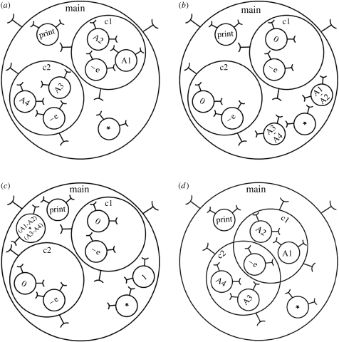
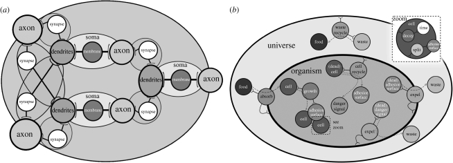
Although SC is designed for biological modelling, it can be used to perform ordinary calculations similar to a conventional computer. Figure 7a–c illustrates the progression of a simple program that performs the nested parallel calculation: PRINT((A1-A2)*(A3-A4)). Note that the subexpression (A1-A2) is performed correctly (instead of A2-A1) because the schemata of the ‘subtract’ system must match the correct systems for the function to be carried out. Figure 7d illustrates the same calculation defined using overlapping scopes to reduce the total number of systems required. (Note that unlike traditional computer approaches, a systemic computer does not add or remove items from memory. Instead, it begins with every system it can support and enables all to interact and be transformed where appropriate. Adding or removing memory or hardware would simply have the effect of adding or removing resources, i.e. systems that are exploited automatically.) Figure 8 illustrates two working models implemented in SC.

Figure 7.

SC calculation of PRINT((A1-A2)*(A3-A4)). As with all SC calculations, interactions occur randomly and asynchronously where permitted by scopes and contexts. The example also demonstrates that SC makes no difference between function and value: the data making up a system may behave as either depending on whether they are interacting or behaving as a context for an interaction. In this figure, the transformation functions of context systems and the results of the transformed systems are written within each system. (a) The initial systems prior to calculation. (b) Systems transformed by subtract–escape function ‘−e’ that subtracts and ejects the result system one level outward, leaving behind the remnant system with a value of zero (executed fragments shown in bold): PRINT((A1-A2)*(A3-A4)). (c) Systems transformed by multiply function producing a system containing the result of the calculation and a remnant containing the value of one, prior to activation of PRINT function which prints the result of the calculation: PRINT((A1-A2)*(A3-A4)). (d) The same calculation can be performed in different ways, for example, a more compact, functionally equivalent arrangement of systems, sharing the subtract–escape function.

Figure 8.

Two simple models constructed using SC: (a) a three-neuron network from Le Martelot et al. (2007a) and (b) a simple organism with metabolism from Le Martelot et al. (2008a).

SC is designed to be written using an intuitive graph-based notation to ease the process of analysis and modelling. It can also be expressed using a calculus notation (see table 1 for details of SC expressions).

Table 1.

SC calculus.

concept	SC calculus notation
system identifier	string
system with internal variable. (Every part of all systems is potentially variable, including parts used for data, schemata and context functions, so all systems may be written as string[x1,x2, …, xi], where i corresponds to the total number of information blocks of the system. However, normally only the variable of interest is written.)	string[x]
system2 partially inside the scope of system1, to degree of n. When n=1, system2 is fully within the scope of system1 and ‘s:n’ may be omitted, reverting to simpler notation. When n=0, system2 is not within the scope of system1 and systems should be written without parentheses. Probability of interaction between systems is dependent on the degree of membership of systems in the same super system. By default, all systems are fully within their own scopes, i.e. systemx(systemx)s:1 for all x	system1(system2)s:n when n=1, use simpler notation system1(system2)s:1⇔system1(system2) when n=0, use simpler notation system1(system2)s:0⇔system1 system2 when both system1 is a member of system2 to degreen1 and system2 is a member of system1 to degree n2: (system1()s:n1system2)s:n2 when n1=0 and n2=0 (system1()s:0system2)s:0⇔(system1()system2)
interacting triplet of system1, system2, context where all three systems are within the same super-scope. All interactions are asynchronous and may occur in parallel with each othera	system1 }-context-{ system2
interacting triplet of system1, system2, context where system2 and context are inside system1. (Assumes system1 is also fully within its own scope. In the special case where system1(system1)s:n and n<1 this interaction is less likely, or when n=0, it is not possible.) All interactions are asynchronous and may occur in parallel with each other	system1(system2) }}-context
‘absorb to (further) degree of m’ interaction rule	system1 }-absorbs:m-{ system2→system1(system2)s:m or system1(system2)s:n }}-absorbs:m→ system1(system2)s:n+m
‘expel to degree of m’ interaction rule	system1(system2)s:n }}-expels:m→ system1(system2)s:n−m
general rule, where system1 and system2 are transformed according to some function or algorithm. (The transformation may also include absorb or expel operations.)	system1 }-context-{ system2→system11 system21 or system1(system2) }}-context→system11(system21)
general rule, where system1 and system2 variables are transformed according to some function f. (The transformation may also include absorb or expel operations.)	system1[x] }-context[f(x,y)]-{ system2[y]→system1[x1] system2[y1] or system1[x] }-context[x,y]-{ system2[y]→system1[x1] system2[y1]
generalized rules, where # indicates ‘any system’ or ‘any variable’, ‘|’ represents ‘or’ and ‘result’ is two transformed systems	system1(#) }}-context→result #(system2) }}-context→result system1 }-context-{ #→result system11 | system12 | system13}-context-{ system2→result
generalized rule, where | indicates ‘or’ (probability of outcome determined by transformation function) and ‘interaction’ is the interacting triplet of system1, system2 and context systems	interaction→system1(system2) | system1 system2 | system2(system1)

^aNote that the same context may be used for any number of pairs of simultaneously interacting systems without conflict as context systems are never changed during the interaction. Conflicts between pairs of interacting systems are not permitted, i.e. system1 }-context1-{ system2 and system1 }-context2-{system3 is not permitted to occur in parallel. (This is based on the assumption that any interacting triplet can be reduced to two sequential interacting pairs.) All other forms of parallelism are unconstrained.

3. Making modelling more intuitive

While mathematicians and computer scientists may enjoy calculus-based representations, it is apparent that many biologists do not. Any modelling and simulation approach must consider the needs of its users in addition to the needs of rigorous and sound hypothesis generation and simulation. SC attempts to satisfy these needs and requirements (tables 2 and 3).

Table 2.

Any language or method to be used for hypothetical mechanism development must have specific features to be valuable for the researcher.

needs for hypothetical mechanism development	matching systemic computation features
be as flexible as possible, to enable complex processes and systems to be defined	SC is a Turing complete computer in its own right (Bentley 2007) and so can simulate all existing computations, software and existing modelsa
ease biologically plausible models, but discourage unnatural or physically implausible models	SC deliberately biases the modeller away from physically impossible models by incorporating conservation of energy, and a requirement for contexts for all interactions, but eases biological modelling by enabling features such as encapsulation, scope, circular causality, parallelism, asynchrony and interaction
enable compact and appropriate descriptions that comprise elements that clearly correlate with and correspond to the elements of the biological system being modelled	SC analysis involves the identification of systems, their interactions and their mutual relationships with each other; experience indicates that the most ‘natural implementations’ tend to be those in which systems correlate well to real physical elements (Le Martelot et al. 2007b)
be readable, both in notational and graphical forms	SC has an intuitive graph-based notation, and a calculus notation that resembles the graph-based notation, making it potentially easier to learn compared with other approaches
enable useful methods of analysis (e.g. formal proofs) of the system being modelled	SC may be analysed formally in the same way as has been achieved using pi-calculus
encourage theorizers to produce hypothetical mechanisms based on the analysis of the natural system and not based on notational ease (or difficulty) of expression	SC is designed to improve models and increase their fidelity, i.e. it makes ‘hacks’ and ‘programmer's tricks’ harder to implement and appropriate descriptions easier

^aAs discussed in Bentley (2007), the notion of Turing completeness is not very useful when viewed in the context of biological modelling—it is perhaps irrelevant whether a human brain is Turing complete or not. However, the notion is relevant in computer science, for it tells us that SC is compatible with all existing computers and simulations. SC may be slow and inefficient at performing conventional serial computations, but it can perform them all; and it is fast and efficient at performing parallel, stochastic computations.

Table 3.

Any simulation package or language to be used for simulation development must have specific features to be valuable for the researcher.

needs for simulation development	systemic computation features
be computationally inexpensive	SC is a parallel computer. Previous work simulated parallelism using a virtual machine (Le Martelot et al. 2007b). Work to create a grid-based SC parallel computer capable of running over any network of computers is underway
enable abstraction at any level of detail	SC forces the modeller explicitly to think about abstraction as they choose what each individual system should model; there are no limits (except those imposed by finite memory of computers) on the level of abstraction or detail that can be supported
enable automated analysis (e.g. statistical, visualization) of the system being simulated	recent research has created a series of visualizers for systemic computation models, allowing information flow, structure and interactions within models to be analysed in detail
enable the hypothetical mechanism under investigation to be exactly simulated	hypothetical mechanisms can be written using the language of SC, then directly run as simulations
ease collaboration between related fields of mathematics, computer sciences and life sciences and enable exploitation of shared knowledge	SC supports bioinspired algorithms (genetic algorithms, neural networks, artificial immune system, developmental algorithms) in addition to more specific biological models, enabling the fields of artificial life, biomimetics, systems biology and computational biology to use the same computational tools

SC is unique, not only because it defines an unconventional (non-Von Neumann) computer architecture, but because it has biases designed to aid in the modelling of natural systems. One such important feature of SC is the incorporation of the law of conservation. In physics, we can informally state ‘the law of conservation’: energy cannot be created or destroyed, it can only be changed from one form to another or transferred from one body to another, the total amount of energy remaining constant (Hiebert 1962).7 In SC this is stated as: systems cannot be created or destroyed, only transformed. It is a fundamental modelling constraint not seen in other modelling or computational approaches. It provides straightforward ‘sanity checking’ of models of natural systems—if the design of a model cannot be implemented in SC because it would require a system to be created or destroyed, then the model is wrong. Practical experience quickly demonstrates how often this constraint is helpful in producing models that obey the laws of physics—which is surely the most fundamental requirement of any model.

For example, in most traditional models of evolution, the death of an organism might result in a system being destroyed and the creation of a new child might involve the creation of a system. In SC (as in reality), the death of an organism simply transforms its state into non-living—its substance still exists and therefore must be dealt with through some form of recycling mechanism (such as an ecosystem). In SC, the creation of a new organism requires the modeller to consider where the substance comprising that organism came from, leading to notions of growth, feeding, nutrients, appropriate movement of nutrients and environment. The repercussions are fascinating—for example, the model of the growing organism shown in figure 8b required food systems to provide the systems needed for growth and metabolism, which were then processed internally, resulting in a turnover of new cells and waste. The waste systems could not be destroyed, so they were recycled in the environment and (eventually) turned back into food again. Perhaps surprisingly, SC thus requires ecologically sound models in order to function properly; otherwise, models may become clogged with waste systems and run out of new systems to process.

While these constraints may be inconvenient for the modeller, they are a fundamental part of our universe and comprise a significant raison d'être for life and why it functions in the way it does. Thus, the simple requirement in SC for transformation (instead of magically appearing or disappearing out of existence like a cartoon) is an important constraint to force the modeller to create more realistic models.

It is hard to prove that any approach is ‘easier to use’ compared with another, or indeed that one methodology is ‘better’ than another. For example, few would argue against the premise that the programming language Prolog is ideally suited for logic-based computations (Bratko 2000), but proving this language is easier or better than another may not be possible. Nevertheless, comparisons can enable more informed judgements.

SC is not the only method capable of expressing biological systems using a graph notation and a calculus. Methods such as stochastic pi-calculus provide an alternative way of expressing biological processes formally. However, the origins of pi-calculus lie in computer science and communications theory (Milner 1993, 2005), where concepts such as ‘channels of communication’ are very important—evident from the non-intuitive method of expressing the interaction and transformation of entities.

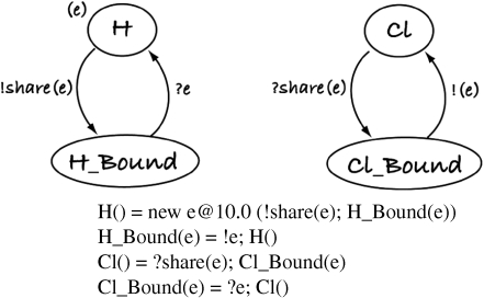
For example, the molecular binding model H+Cl↔HCl shows the difference in clarity of expression very clearly. Figure 9 shows the extremely simple stochastic pi-calculus model (hypothetical mechanism) used by Phillips & Cardelli (2004) to introduce and teach stochastic pi-calculus. Atom H donates its electron, which is shared between H and Cl. Cl then loses an electron and H gains it to break the bond. But despite its simplicity, the model is confusing. The use of non-intuitive symbols makes reading the graph notation and the calculus a challenge. Even worse, in the model, binding of H and Cl is never explicit—they are never actually linked in the model, simply transformed from H to H_Bound and Cl to Cl_Bound. It is also unclear at what level of abstraction this model uses as it contains both atoms (which comprise electrons, neutrons and protons) and one electron. This combination of non-intuitive notation (what does ‘?’ and ‘!’ mean?), confusion of bindings (which atom is bound to which?) and a confusion of abstractions (are atoms being modelled or electrons, protons and neutrons?) results in a partial and somewhat cryptic model.

Figure 9.

Graphical representation of pi-calculus model and the corresponding notation of binding model H+Cl↔HCl (adapted from Phillips & Cardelli 2004). It is not obvious that H and Cl become bound to each other, despite this being the purpose of the model.

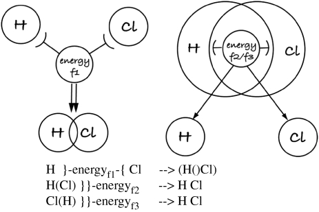
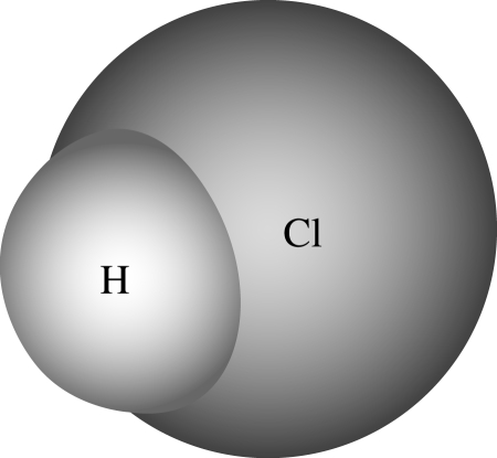
By contrast, when using SC, we have no need for such complications; instead we can remain at one level of abstraction—the atom. We do not need to model individual electrons for such a simple model of binding. All we need to do is to ensure the scopes of each atom overlap. The result in SC graph form (figure 10) looks similar to a familiar representation of the molecular model for HCl (figure 11), making the model remarkably intuitive and simple to understand. But most significantly, the SC version includes the cause of the binding—energy. The whole reaction between the two atoms is impossible without sufficient energy—a detail that is necessary to include in SC (the interaction between the atoms must occur in some context) but can be and has been ignored in pi-calculus, resulting in an incomplete model. In addition, while ease of understanding is always a subjective measure, a comparison between figure 9 (duplicated from a tutorial on how to teach pi-calculus, by Phillips & Cardelli (2004)) and the same model (hypothetical mechanism) implemented in SC in figure 10 shows clear evidence that SC is more descriptive and representative of reality and uses simpler calculus notation.

Figure 10.

SC graph model and the corresponding notation of binding model H+Cl↔HCl. Note that the diagram closely resembles standard diagrammatic representations of this chemical process (figure 11) and clearly shows how H and Cl become bound in a symmetrical way.

Figure 11.

Molecular model of HCl (hydrogen chloride).

Both SC and pi-calculus enable multiple atoms and bindings to be modelled by the addition of parameters. But SC permits the modelling of this process in more detail by revealing the deeper systems (protons, neutrons and electrons) hidden within the H and Cl systems without changing the overall structure of the model. It should thus be evident that by designing SC explicitly for natural and biological computations, real advantages of clarity can be obtained compared with other modelling approaches.

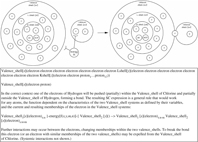
One of the advantages of SC is that it encourages modellers to understand and investigate the systems they are modelling. If a ‘context system’ has a complex function, then it may well abstract the behaviours of several underlying systems (e.g. in this example model, the ‘energy context’ must comprise sufficient ionization energy to push an electron outside the potential barrier of one atom and into another—and the specific amount of energy depends on how many other electrons and neutrons are present). This might lead to a further development of the model (hypothetical mechanism), incorporating the shell theory (figure 12).

Figure 12.

An overview of the HCl binding model at a lower level of abstraction using SC.

One final advantage of SC is that it is more than a language. It defines a parallel, stochastic computer that is designed to behave in a manner more akin to biological systems compared with conventional computers (Bentley 2007; Le Martelot et al. 2007b). This means that when a systemic computer is being used to model a biological system with fault tolerance and self-repair, these biological features are enabled without the brittle nature of conventional computers and operating systems causing difficulties (Le Martleot et al. 2008a). (Previous work has demonstrated that while conventional computers modelling evolutionary developmental systems may enable the systems to recover from 1 per cent damage, a systemic computer modelling evolutionary developmental systems can recover from over 33 per cent damage. The difference was caused by conventional operating systems failing in the former case (Bentley 2005; Le Martelot et al. 2008b).)

4. Deliberately incorrect modelling: the use of substitution

SC is designed to aid modellers and improve their ability to determine an appropriate level of abstraction for their models. But whether SC is used or not, abstraction is a vital notion when modelling. Which elements should be accurately represented, which should be approximated by a simpler component or which should be ignored altogether? The rule of thumb, ‘model the elements that have the most effect and simplify or ignore everything else’, is often our only option.

However, there are times when we wish to model an important element with some precision, but are prevented from doing so because of the extreme computational demands. In such cases, modellers often choose approximation, resulting in a model with decreased accuracy and disappointing predictive capabilities. However, there are other ways to design models. Instead of attempting to replace an element with a simpler approximation, it is sometimes possible to substitute the element with a different but functionally similar component.

To illustrate this principle, the final part of this paper provides an example of a model based on substitution—the fractal GRN (Bentley 2004a). In this work, the focus of investigation was on the evolution of GRNs that had specific patterns of gene activation. Previous models that made use of simplified and often binary gene–protein interactions (de Garis 1999; Reil 2003; Kumar 2004; Basanta 2005; Gordon 2005) showed disappointing evolvability that prevented desirable or complex solutions from evolving. None of the models attempted to include the more complex chemical interactions caused by protein folding and protein interactions. A hypothesis was formed:

when more complex chemistries are available to evolution, evolvability is greater,

i.e. the larger the number of possible protein shapes, the more possible interactions there could be between proteins, and so the more possible ways for evolution to enable genes to interact with each other. This hypothesis was in direct opposition to conventional wisdom in optimization theory, which suggested that fewer possible solutions make the search for a desired solution easier (Goldberg 1989).

It is not possible to test this hypothesis in the wet laboratory for we cannot easily alter biochemistries and force life to use ultra-simple chemistries and then perform thousands of evolutionary experiments. Thus it is an ideal candidate for computational modelling. But a hypothesis of this type presents unique problems for simulation development. Just as it is difficult to simplify biochemistries of living organisms, it is difficult to complexify computer models. An evolutionary model requires millions of individual solutions to be evaluated, each comprising thousands or millions of protein interactions even for a small GRN. Since evolution would be designing new proteins, some way of calculating how they each interacted would be required. Modelling protein folding with enough accuracy or speed to allow realistic artificial chemistries to be embedded in such a simulation is infeasible, even with the fastest of contemporary computers. But if complex chemistries cannot be modelled, how can the hypothesis be tested in simulation?

The solution is substitution. Instead of attempting to model real protein folding, the concept can be substituted with a process of complex shape formation taken from mathematics—fractals. This was the solution used for the study (Bentley 2004a–c, 2005). A model was created in which genes were parameters which mapped to subsets of the Mandelbrot set. Proteins were thus represented by fractal shapes of infinite complexity, with the number of possible shapes limited only by the precision of the computer and the equation of the fractal. Proteins were permitted to interact according to their shapes, and with matching fractal cis-sites of genes. This solution was a computational trick—fractals are fast and easy to compute—but the result was an infinitely complex fractal chemistry with many of the same properties of biochemistry. (For example, fractal proteins are not random—the self-similarity of fractals means that some shapes are more common than others; but there is an infinite number of variations of similar shapes.) The model does not suggest that biology is fractal (although some researchers do appear to claim this; Mitra & Rani 1993); it merely uses substitution to enable similar properties to be produced more feasibly and practically than would otherwise be possible.

Currently in this model, there exist the following.

• —Fractal proteins, defined as subsets of the Mandelbrot set. In this work, four categories of proteins are modelled: those within the cell cytoplasm (cfractal protein); those used within the cell for cell behavioural and structural purposes (bfractal proteins); those outside the cell (efractal proteins); and those that behave as cell receptors to enable transport of environmental proteins inside the cell (rfractal proteins). Multiple fractal proteins of the same type are merged into a fractal compound, whose shape depends on the fractal shapes of the constituent fractal proteins.

• —Environment, which can contain one or more fractal proteins (expressed from the environment gene(s)), and one or more cells.

• —Cell, which contains a genome and cytoplasm, and which has some behaviours.

• —Cytoplasm, which can contain one or more fractal proteins.

• —Genome, which comprises structural genes and regulatory genes. In this work, the structural genes are divided into different types: cell receptor genes; environment genes; and behavioural genes.

• —Regulatory gene, comprising operator (or promoter) region that may be activated or suppressed by a matching cfractal protein compound and coding (or output) region, which produces a cfractal protein.

• —Cell receptor gene, a structural gene with a coding region which produces an rfractal protein that acts as a mask, permitting variable portions of the environmental proteins to enter the corresponding cell cytoplasm.

• —Environment gene, a structural gene that determines which efractal proteins (maternal factors) will be present in the environment of the cell(s).

• —Behavioural gene, a structural gene comprising operator region and a cellular behaviour region, which produces bfractal proteins.

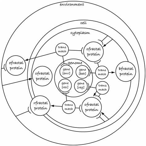
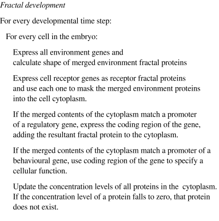
Figure 13 illustrates the representation using SC. Figure 14 provides an overview of the algorithm used to develop a phenotype from a genotype. Note how most of the dynamics rely on the interaction of fractal proteins. Evolution is used to design genes that are expressed into fractal proteins with specific shapes, which result in developmental processes with specific dynamics. Figure 15 illustrates how two fractal proteins can interact and form a new fractal compound shape, which has a shape and concentration dependent on the fractal shape of its constituents. The fractal compound is formed by merging fractals. Fractal proteins are merged (for each point sampled) by iterating through the fractal equation of all proteins in ‘parallel’, and stopping as soon as the length of any is unbounded (i.e. greater than 2). Intuitively, this results in black regions being treated as though they are transparent, and paler regions ‘winning’ over darker regions. Other types of protein have different effects, e.g. receptors act as masks on environmental proteins (Bentley 2004a–c). In this way, fractal proteins interact together forming new compounds that alter the expression of genes, which produce new fractal proteins, and so on, in a highly complex fractal chemistry.

Figure 13.

Fractal GRN model in SC graph notation, using ‘trans mach’ (transcription machinery) systems to enable the gene–protein interactions.

Figure 14.

The fractal development algorithm written as conventional pseudocode for clarity. (SC notation can be provided on request by the author; however, the complexity of this model means that the description is lengthy and beyond the scope of this paper.)

Figure 15.

(a,b) Two fractal proteins and (c) the resulting merged fractal protein compound.

Interested readers can find complete details of the experiments performed using this model in Bentley (2004a–c, 2005). In summary, experiments showed that using this model evolution was able to evolve a series of GRNs that produced many desired patterns of gene activation, including sequential counting behaviours (Bentley 2004a). Surprisingly, however, unlike simpler models of genes and proteins, in this simulation, evolution never ceased in its fine-tuning of the solutions. Even when perfect fitness scores were achieved (patterns of activation that matched the desired patterns perfectly), evolution continued to alter the genes and corresponding protein shapes to satisfy unspecified secondary goals of efficiency and robustness to enable these good solutions to survive further disruption by evolution. In other words, as an unexpected side effect of the evolvability of this model, the evolutionary algorithm that generated fractal GRNs within the developmental process had a natural tendency towards the creation of efficient and compact solutions by reducing the number of genes and proteins employed within solutions. The same system also had a natural tendency towards more robust solutions (genetic canalization), increasing the ability of GRNs to survive damage from the removal of genes (Bentley 2004b). This effect was investigated further by using the model to evolve and develop a computer program, which was then deliberately damaged to assess its ability to survive—akin to damaging phenotypes and assessing viability (Bentley 2005). The program displayed graceful degradation and continued to function (compared with a human-designed program and an evolved program not using the fractal protein model, which failed instantly and fatally at the smallest corruption; Bentley 2005). The same model has even been shown to be capable of evolving fractal GRNs of sufficient complexity to guide a robot through a maze (Bentley 2004c), while other researchers have also corroborated the findings by reimplementing the same model and showing improved evolvability compared with other approaches (Zahadat & Katebi 2008).

Substituting fractals for an infeasible biologically accurate model of protein folding and biochemistry is just one way of investigating a natural phenomenon through careful simulation design. But care must be taken to identify the level of abstraction involved, the systems to be modelled, their interactions and organization, before any attempt at substitution is made.

5. Lessons for biological modelling

Modelling and simulation is still something of a black art. While many researchers are trained in experimental design and statistical analysis, the majority of biology modellers are self-taught because of the interdisciplinary nature of the work. The result can be a mixture of mathematical and software models, not fully understood by biologists and potentially not incorporating the very concepts they are supposed to help analyse. While not every researcher may be comfortable with using SC or fractal proteins for their application, lessons learned from the use of these techniques can be exploited by all those with an interest in modelling. These are summarized below.

1. Identify the scope of your work. Referring back to figure 1, explicitly identify which biological system is to be the subject of study and which behaviour is of relevance. This is often best performed by examining the availability of data—the more reliable the data that are available, the better the model will be. This should not just be data describing the biological behaviour; it should be as much data as possible on the nature and workings of the biological system itself, its constituents and interactions between them.

2. Explicitly state your hypothetical mechanism: how do you believe the biological system is working; what assumptions are you making; what predictions can you make about the behaviour if your hypothesis is correct; and are there any behaviours that, if observed, would disprove your hypothesis? Again, this should be stated with as much detail as you can.

3. Design the simulation (which if using SC you will be doing as you state your hypothetical mechanism above). A simple design is often easier and desirable, but not always better—biology is not simple and so the simplest models may lack significant detail. Ensure that you do the following.

   1. Define the level of abstraction and try to represent everything at that level. If you are trying to model tumour development, you may want to model cells and some genes and proteins—you do not need to model electron clouds around atoms, or populations of evolving organisms. Or if you are modelling an ecology, you may model populations of organisms and weather patterns, but you can ignore cells and proteins. However, do not forget that all of these features exist in reality and may form the context that modifies the interaction of entities at the level of abstraction you have chosen. The decision of which level of abstraction to use is often determined by the amount of data available and the feasibility of computation.
   2. Identify the features to be modelled. In SC, this equates to identifying the systems. So if modelling tumours: which cells will be included in the model; which genes; and which proteins? These may include some very fundamental features such as the laws of physics, Brownian motion or reflectance of light. The normal rule of thumb is to include those systems that have the most effect. But everything not explicitly modelled may still have an effect, so try to state and justify what is not in the model in addition to what is in it.
   3. Identify the organization of the features. In SC, this corresponds to specifying the scopes of systems: which systems are able to affect others and which are not; which contain subsystems or may subsume or expel systems in the future; and how are systems physically arranged in relation to each other?
   4. Identify the interaction of the features. In real life, nothing happens without some interaction. The most revealing models are those that produce behaviours because of the interaction of their constituents, for such models provide better explanations for the cause of those behaviours. (For example, a numerical model that describes evolutionary dynamics with a single equation may be very useful, but a model that describes evolutionary dynamics through modelling of interacting individuals allows the analysis of how dynamics correspond to detailed changes in individuals, their number and their interactions.)

4. Implement the simulation. If any significant element is excessively computationally expensive, consider substituting the element with a behaviourally equivalent analogue (e.g. fractals for protein folding). If the design is still infeasible, change the level of abstraction and redesign the model. A good model should be transparent, intuitive and unambiguous—it should be obvious how it works, what it represents and thus easily extendible. It should be straightforward to monitor and should produce as much data as possible and feasible.

5. Test the simulation. First, is its representation appropriate? In SC, does each system correspond to something real in the biological system (or does it represent a programmer's short cut)? Second, does the simulation behaviour correspond to the behaviour you hypothesized, and does it correspond to the behaviour of the biological system under study? If not, check the design and hypothesis. The aim is not to modify the simulation iteratively until it behaves as you wish—the aim is to find a valid hypothesis that can be tested by comparing the behaviour of simulation with reality. For example, a simple electronic calculator may accurately reproduce the ability of our brains to perform addition, but while this aspect of its behaviour may be similar, it provides no explanation of how our brains work. A hypothesis that a network of neurons in our brains can learn to perform addition, tested by a simulation of a neural network that successfully adds numbers together, provides a much more convincing explanation.

6. Finally, use the simulation to test the hypothetical mechanism. Does its behaviour match the behaviour of the biological system; if you alter the model in specific ways, can the new behaviour (a prediction made by the model) be verified by running new experiments in the biological system; does the model match new previously unseen biological data for the system under study; can the analysis of the inner mechanisms of the model be used as predictors in the biological system; and do new findings about the inner mechanisms in the biological system correspond to the behaviour of the internal systems in the model?

SC is one approach that has been designed to aid the modelling process and encourage modellers to follow the lessons listed above. Future work will continue to develop this method by creating a fully parallel systemic computer and releasing the SC language, compiler and visualizer for general use.

6. Summary

All models are incorrect. The most important aspect of modelling is to follow a clear design methodology that will help highlight unwanted deficiencies. Even before beginning, the modeller should be aware of the fundamental questions: how will the hypothetical mechanism be assessed for accuracy; how can the simulation be checked to guarantee it follows the hypothetic mechanism; and how are the resulting behaviours compared which each other, and with biological reality?

Most ‘artificial life’-based models use combinations of different algorithmic techniques, from object-oriented, to process-driven, to iterative rewriting grammars. There is no coherent methodology available for correlating these programmer's tricks with real, physical biological entities and indeed most modellers make no attempt to do so (Webb 2001). This results in opaque and largely unsubstantiated models that rely on subjective metaphors and wishful thinking to provide relevance for biology.

There can be no final answers or definitive solutions to the problem of modelling, just as there can be no single experimental approach or programming style that will suit all situations. Nevertheless, the use of tools designed to aid the modelling process can be of benefit in many situations. In this paper, the modelling approach called SC was introduced. SC is an interaction-based language, which enables individual-based expression and modelling of biological systems, and the interactions between them. SC permits a precise description of a hypothetical mechanism to be written using an intuitive graph-based notation or a calculus-based notation. The same description can then be directly run as a simulation, merging the hypothetical mechanism and the simulation into the same entity. In this approach, all that is required is to ask three questions (repeatedly): do the entities in the model correspond to clear and measurable entities in reality; are the entities in the model organized in the same way compared with their corresponding entities in reality; and do the interactions and results of interactions between modelled entities correspond to the interactions and results of interactions in reality?

Despite our best efforts to produce good models, the best model is not always the most accurate one. Frequently, computational constraints or lack of data make it infeasible to model an aspect of biology. Simplification may provide one way forward, but with inevitable consequences of decreased accuracy. Instead of attempting to replace an element with a simpler approximation, it is sometimes possible to substitute the element with a different but functionally similar component. In the second part of this paper, one such model was summarized: the fractal protein model and its advantages were summarized.

As advances in fields such as synthetic biology continue to be made, the needs for modelling and simulation become ever greater. It can be argued that biology is an example of a macroscale nanocomputer, designed by evolution to exploit behaviours from subatomic to ecological. If we stand any chance of exploiting and redesigning biology, new advances in modelling languages, computers and methodologies are required. Our models will always be wrong—the trick is to design them that way on purpose.

References

- Adamatzky A. (ed.) 2002. Collision-based computing, vol. XXVII, p. 556 London, UK: Springer. [Google Scholar]
- Basanta D. 2005. Using genetic algorithms to evolve microstructures. PhD thesis, Kings College London, London, UK. [Google Scholar]
- Bentley P. J. 2004a. Fractal proteins. J. Genet. Program Evol. Mach. 5, 71–101. ( 10.1023/B:GENP.0000017011.51324.d2) [DOI] [Google Scholar]
- Bentley P. J. 2004b. Evolving beyond perfection: an investigation of the effects of long-term evolution on fractal gene regulatory networks. BioSystems. 76, 291–301. ( 10.1016/j.biosystems.2004.05.019) [DOI] [PubMed] [Google Scholar]
- Bentley P. J. 2004c. Controlling robots with fractal gene regulatory networks. In Recent developments in biologically inspired computing (eds de Castro L., von Zuben F.). Hershey, PA: Idea Group Inc [Google Scholar]
- Bentley P. J. 2005. Investigations into graceful degradation of evolutionary developmental software. J. Nat. Comput. 4, 417–437. ( 10.1007/s11047-005-3666-7) [DOI] [Google Scholar]
- Bentley P. J. 2007. Systemic computation: a model of interacting systems with natural characteristics. Int. J. Parallel Emerg. Distrib. Syst. 22, 103–121. ( 10.1080/17445760601042803) [DOI] [Google Scholar]
- Blain D., Garzon M., Shin S.-Y., Zhang B.-K., Kashiwamura S., Yamamoto M., Kameda A., Ohuchi A. 2004. Development, evaluation and benchmarking of simulation software for biomolecule-based computing. Nat. Comput. 3, 427–442. ( 10.1007/s11047-004-2644-9) [DOI] [Google Scholar]
- Bratko I. 2000. Prolog programming for artificial intelligence. Reading, MA: Addison Wesley [Google Scholar]
- Bullock S., Noble J., Watson R., Bedau M. A. (eds) 2008. Artificial life XI. In Proc. 11th Int. Conference on the Simulation and Synthesis of Living Systems Cambridge, MA: MIT Press. [Google Scholar]
- Cardelli L. 2005. Brane calculi—interactions of biological membranes. In Computational methods in systems biology (CMSB'04). LNCS, vol. 3082, pp. 257–280. Berlin, Germany: Springer. [Google Scholar]
- Chan K. H., Tidwell P. M. 1993. The reality of artificial life: can computer simulations become realizations? In Third International Conference on Artificial Life. [Google Scholar]
- de Garis H. 1999. Artificial embryology and cellular differentiation. In Evolutionary design by computers (ed. Bentley P. J.), ch. 12, pp. 281–295. London, UK: Academic Press. [Google Scholar]
- Dupuy L., Mackenzie J., Rudge T., Haseloff J. 2007. A system for modelling cell–cell interactions during plant morphogenesis. J. Ann. Bot. 101, 1255–1265. ( 10.1093/aob/mcm235) [DOI] [PMC free article] [PubMed] [Google Scholar]
- Eriksson D. 1997. A principal exposition of Jean-Louis Le Moigne's systemic theory. Rev. Cybernet. Hum. Knowing. 4, 2–3. [Google Scholar]
- Goldberg D. E. 1989. Genetic algorithms in search, optimization and machine learning. Boston, MA: Addison-Wesley; Longman Publishing Co., Inc [Google Scholar]
- Gordon T. 2005. Exploiting development to enhance the scalability of hardware evolution. PhD thesis, Department of Computer Science, University College London, London, UK. [Google Scholar]
- Hiebert E. N. 1962. Historical roots of the principle of conservation of energy. Madison, WI: University of Wisconsin Press [Google Scholar]
- Holmes W. R., Jung R., Roberts P. 2008. Computational neuroscience (CNS*2008). BMC Neurosci. 9(Suppl. 1), I1 ( 10.1186/1471-2202-9-S1-I1) [DOI] [PMC free article] [PubMed] [Google Scholar]
- Juang J.-N. 1993. Applied system identification. Upper Saddle River, NJ: Prentice Hall PTR [Google Scholar]
- Kumar S. 2004. Investigating computational models of development for the construction of shape and form. PhD thesis, Department of Computer Science, University College London, London, UK. [Google Scholar]
- Le Martelot E., Bentley P. J., Lotto R. B. 2007a. Exploiting natural asynchrony and local knowledge within systemic computation to enable generic neural structures. In Proc. Int. Workshop on Natural Computation (IWNC 2007), Nagoya, Japan, 10–13 December 2007. [Google Scholar]
- Le Martelot E., Bentley P. J., Lotto R. B. 2007b. A systemic computation platform for the modelling and analysis of processes with natural characteristics. In Proc. Genetic and Evolutionary Computation Conference (GECCO 2007) Workshop: Evolution of Natural and Artificial Systems—Metaphors and Analogies in Single and Multi-Objective Problems, pp. 2809– 2816. [Google Scholar]
- Le Martelot E., Bentley P. J., Lotto R. B. 2008a. Crash-proof systemic computing: a demonstration of native fault-tolerance and self-maintenance. In Proc. 4th IASTED International Conference on Advances in Computer Science and Technology (ACST 2008), Langkawi, Malaysia, 2–4 April 2008. [Google Scholar]
- Le Martelot E., Bentley P. J., Lotto R. B. 2008b. Eating data is good for your immune system: an artificial metabolism for data clustering using systemic computation. In Proc. 8th Int. Conference on Artificial Immune Systems (ICARIS 2008) Springer LNCS, vol. 5132, pp. 412–423. [Google Scholar]
- McMullin B., Varela F. J. 1997. Rediscovering computational autopoiesis. In Proc. European Conference on Artificial Life (ECAL 1997), Brighton, UK, July 1997. [Google Scholar]
- Milner R. 1993. The polyadic pi-calculus: a tutorial. In Logic and algebra of specification (eds Hamer F. L., Brauer W., Schwichtenberg H.), pp. 203–246. Berlin, Germany: Springer. [Google Scholar]
- Milner R. 2005. Axioms for biographical structure. J. Math. Struct. Comput. Sci. 15, 1005–1032. ( 10.1017/S0960129505004809) [DOI] [Google Scholar]
- Mitra C. K., Rani M. 1993. Proteins sequences as random fractals. J. Biosci. 18, 213–220. ( 10.1007/BF02703118) [DOI] [Google Scholar]
- Nelles O. 2000. Nonlinear system identification: from classical approaches to neural networks and fuzzy models. Berlin, Germany: Springer [Google Scholar]
- Phillips A., Cardelli L. 2004. Simulating biological systems in the stochastic pi-calculus (introductory tutorial). Cambridge, UK: Microsoft Research [Google Scholar]
- Reil T. 2003. Artificial genomes as models of gene regulation. In On growth form and computers (eds Kumar S., Bentley P. J.), London, UK: Academic Press [Google Scholar]
- Rudge T., Haseloff J. 2005. A computational model of cellular morphogenesis in plants. J. Adv. Artif. Life. 3630, 78–87. ( 10.1007/11553090_9) [DOI] [Google Scholar]
- Stepney S., Smith R. E., Timmis J., Tyrrell A. M., Neal M. J., Hone A. M. W. 2005. Towards a conceptual frameworks for artificial immune systems. Int. J. Unconventional Comput. 1, 315–338. [Google Scholar]
- Varela F. J., Maturana H. R., Uribe R. 1974. Autopoiesis: the organization of living systems, its characterization and a model. BioSystems. 5, 187–196. ( 10.1016/0303-2647(74)90031-8) [DOI] [PubMed] [Google Scholar]
- Webb B. 2001. Can robots make good models of biological behaviour?. Behav. Brain Sci. 24, 1033–1050. ( 10.1017/S0140525X01000127) [DOI] [PubMed] [Google Scholar]
- Wheeler M., Clark A. 1999. Genic representation: reconciling content and causal complexity. Br. J. Philos. Sci. 50, 103 135 ( 10.1093/bjps/50.1.103) [DOI] [Google Scholar]
- Wren J. D., Wilkins D., Fuscoe J. C., Bridges S., Winters-Hilt S., Gusev Y. 2008. In Proc. 2008 MidSouth Computational Biology and Bioinformatics Society (MCBIOS) Conference. BMC Bioinf. 9(Suppl. 9), S1 ( 10.1186/1471-2105-9-S9-S1) [DOI] [PMC free article] [PubMed] [Google Scholar]
- Xinshu X., Thomas M. J., Ramakrishna M. 2005. System identification: a multi-signal approach for probing neural cardiovascular regulation. Physiol. Measurement. 26, R41–R71. ( 10.1088/0967.3334/26/3/R01) [DOI] [PubMed] [Google Scholar]
- Zahadat P., Katebi S. D. 2008. Tartarus and fractal gene regulatory networks with input. Adv. Complex Syst. 11, 803–829. ( 10.1142/S0219525908001982) [DOI] [Google Scholar]