Improving initial polyp candidate extraction for CT colonography

Abstract

Reducing the number of false positives (FPs) as much as possible is a challenging task for computer-aided detection (CAD) of colonic polyps. As a part of a typical CAD pipeline, an accurate and robust process for segmenting initial polyp candidates (IPCs) will significantly benefit the successive FP reduction procedures, such as feature-based classification of false and true positives (TPs). In this study, we introduce an improved scheme for segmenting IPCs. It consists of two main components. One is geodesic distance-based merging, which merges suspicious patches (SPs) for IPCs. Based on the merged SPs, another component, called convex dilation, grows each SP beyond the inner surface of the colon wall to form a volume of interest (VOI) for that IPC, so that the inner border of the VOI beyond the colon inner surface could be segmented as convex as expected. The IPC segmentation strategy was evaluated using a database of 50 patient studies, which include 100 scans at supine and prone positions with 84 polyps sized from 6 to 35 mm. From each VOI, several widely-used features were extracted and fed into a support vector machine classifier for the classification of TPs and FPs. The presented IPC segmentation strategy demonstrated improvement, in terms of having no undesirably merged true polyp and providing more helpful mean and variance of the image intensities of IPCs for the classification of the TPs and FPs, as compared to our previous method.

I. Introduction

According to the up-to-date statistics from American Cancer Society (ACS) [1], colorectal cancer ranks the third most common occurrence of both cancer deaths and new cancer cases in 2008 for both men and women in the United States. Fortunately, early detection and removal of colonic polyps prior to their malignant transformation can effectively decrease the incidence of colon cancer [2]. As a potential minimally-invasive screening technique, computed tomographic colonography (CTC) or CT-based virtual colonoscopy (VC) has shown several advantages over the traditional optical colonoscopy (OC) [3]. To improve the efficiency of CTC in detecting polyps, computer-aided detection (CAD) of polyps has shown the potential of being a second reader assisting physicians for finding polyps in the colon [4].

Generally, starting from a segmented colon wall, most of the current CAD schemes detect initial polyp candidates (IPCs) represented by a group of voxels, i.e., a volume of interest (VOI), based on which the CAD schemes conduct feature analysis for the purpose of reducing false positives (FPs) [5]. To generate the IPCs, several techniques have been reported. Firstly, voxels on the colon wall with a possibility of being part of a polyp candidate were labeled or filtered, based on various heuristic rules like curvature [6, 7], shape index and curvedness [8–10], HT (Hough transformation)-score [11], and surface normal overlap [12] in a certain value range. These voxels were then clustered based on the spatial adjacency to form suspicious patches (SPs). Since multiple SPs might be generated for one colonic object, SPs which are close but not connected to each other were merged if the Euclidian distance (ED) between them was less than a predefined threshold [8–11, 13, 14, 15]. Finally, the VOIs of IPCs were generated with different methods. For example, in [6, 12, 16], the SPs were directly utilized as the VOIs. Alternatively, a cubic or rectangular sub-volumes centered at the centroid of such un-merged [7] or merged [10, 11] SPs were assumed as the VOIs of IPCs for the purpose of including more voxels of the polyp candidates. To reduce the redundant voxels in the above sub-volumes, non-rectangular volume areas created by sphere fitting [17], three-dimensional (3D) surface fitting [18] and ellipsoid fitting [13] were explored. However, some lumen voxels might still be included in such fitted volume area. Loyal to the truth that the contrast at the SP-lumen interface (outer border) is conspicuous enough to be detected reliably, several researchers have been focusing on constructing the interface between the polyp candidates and the normal tissue (inner border) for an adequate VOI of IPC. For example, some researchers grew the SPs towards tissue area with region growing techniques, like conditional morphological dilation [9], while others believed that the contrast at the interface of polyp candidates and normal tissue was strong enough for them to find the inner border by the use of edge-detectors like Harr transform-based edge finder [13, 14], a combination of canny edge detection and Radon transform [19], deformable models like the curvature-driven level set evolution [20] and the active contour model [7].

For adequate VOI extraction, correct merging of SPs and accurate segmentation of the inner border would be critical but still problematic. The merging criteria employed in the above methods are all based on the ED. However, the ED cannot serve as the criteria alone to determine whether multiple SPs belong to one object or not, since ED ignores the height information of SPs. Therefore, we introduce a geodesic distance (GD)-based merging (GDM) strategy in this study to address this problem. Additionally, in CTC images, the image contrast between a polyp and its surrounding normal tissue could be too small to be detected by those edge-detectors [7, 13, 14, 19, 20]. On the other hand, the morphological dilation method [9], though it did not use any edge-detector, might generate concave inner border [14], while the inner border is often expected to be flat or convex [21]. Therefore, we introduce a convex dilation (CD) strategy to ensure that a flat and/or convex inner border will be generated for the final VOI of each IPC, and we hope such VOI can benefit the successive FP reduction procedures. The presented GDM and CD strategies are adapted to our previous CAD pipeline [14] and then evaluated using a CTC database.

The remainder of this paper is organized as follows. Section 2 introduces the two strategies for VOIs of IPCs. Section 3 reports the evaluation results. Several conclusions are drawn in Section 4 through some discussions.

II. Method

To facilitate the presentation of the two strategies, the whole CAD scheme is outlined in Fig. 1. At the beginning, voxels are labeled and clustered based on spatial adjacency to form the SPs (the details are given, e.g., in [14]). These SPs are merged with the GDM strategy and then grow towards the inner border with the CD strategy. To evaluate the strategies, several widely-used features are extracted from the generated VOIs of the IPCs and fed into the well-known support vector machine (SVM) for FP reduction.

Fig. 1.

The outline of a CAD scheme to evaluate the presented two strategies.

2.1 Geodesic distance-based merging (GDM) strategy

Frequently, multiple SPs can be generated for one polyp candidate, especially for those lobulated ones. Fig. 2 shows an example of three SPs being generated for a 35 mm lobulated tubulovillous adenoma. Therefore, SPs located within a merging distance L_m, which was the ED like 12.5 mm in [8–10, 14, 15] and 10 mm in [11], were merged together as one. However, two or more unrelated SPs may be mistakenly merged. Fig. 3(a) shows an example of stool standing closely to a polyp in the same colon segment, while Figs. 3(b, c, and d) show another example of stool locating closely to a polyp in different segments of the colon. Each of the two stools in Fig. 3 is merged to the related polyp to form two IPCs if L_m is set to be 12.5 mm, which will undoubtedly impair the performance of the following FP reduction.

Fig. 2.

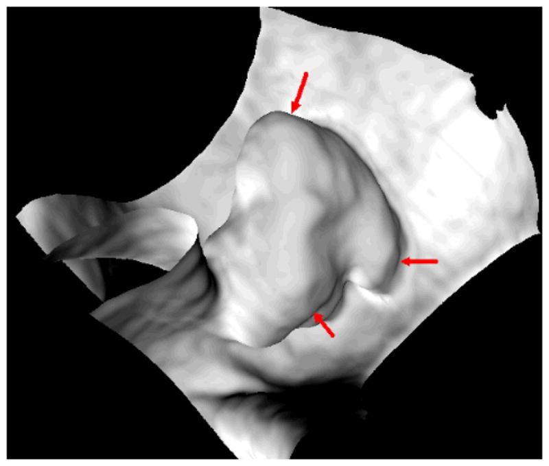
The endoluminal or endoscopic view of a 35 mm lobulated tubulovillous adenoma near the rectum of a 54-year old female. The three arrows indicate three separated SPs, respectively, which are detected for this single polyp due to the three lobules.

Fig. 3.

(a) The endoluminal view of a 9 mm polyp and stool which are close to each other. (b) A 6 mm polyp and stool in the 2D axial slice. Obviously, they are located in different segments of the colon. (c) The endoluminal view of the two colonic objects in (b), where the view angle is set mainly for the polyp. (d) Similar to (c), but at another view angle for the stool.

The reason for such undesirable merging lies in that the ED between the two objects just reflects their smallest spatial distance, but ignores the height information of the objects standing out of their surroundings. Such conjecture can be illustrated by the 2D pictures in Fig. 4, where both the EDs from P1 to P2 and from P3 to P4 are smaller than the merging distance L_m of 12.5 mm and, therefore, P1 and P3 shall be merged with P2 and P4, respectively, according to the previous works [8–10, 14, 15]. By inspecting these two pictures in Fig. 4, we would conclude that the ED from P3 to P4 is similar to that from P1 to P2, however, their relative larger heights make them much more likely to be different objects (P3 and P4) standing on the underlying major object (the dark circle in Fig. 4) than other two objects (P1 and P2). The SPs P1 and P2 appear more likely to be lobules of their underlying major object (the dark circle) and may be merged, but P3 and P4 should not be merged.

Fig. 4.

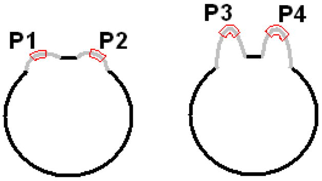
The two dark circles represent two major objects, on which there are two bumps (mimicking polypoid-like objects) in light gray respectively. Parts of the bumps encompassed by the red curves are the peak and neck areas of the objects, denoted by P1 to P4, which represent the SPs detected by an analysis on each voxel on the borders of the major objects.

Based on the above analysis, we notice that the height of the SPs should also be considered in the merging process. The GD between any two points on a manifold (the colon wall in this study) is the length of the shortest path on the manifold connecting them, i.e., the geodesic path [22]. In Fig. 4, the geodesic paths from P1/P3 to P2/P4 are the gray and dark curves rather than the straight lines (EDs) connecting them, whose lengths (GDs) reflect the height information of the SPs according to the underlying major object. Therefore, we introduce a GDM strategy to improve the SP merging process. Fig. 5 shows a flow chart for the GDM strategy, where L_ED and L_GD denote the ED and GD respectively between any two SPs. Notation γ represents a constant threshold. The first condition inherits the criteria of the previous works [8, 14, 15]. The second criteria is introduced here for the rationale that if the ratio of the GD to ED between any two SPs is small enough (the values of GD and ED are similar), the height of the patches would be relative small and they should be conceptually considered as lobules of one object; otherwise, they would be different objects and shouldn’t be merged.

Fig. 5.

A flow chart for the GDM strategy.

The GD can be computed accurately using Dijkstra method [23] if taking the manifold as a graph [22]. In this study, for simplicity, the GD is approximated by the number of steps (denoted with n_D) of a geodesic dilation, which starts from one SP and ends at another with the dilation process limited only on the colon wall. After applying the geodesic dilation with n_D steps, the generated geodesic path would be a sequence of n_D+1 voxels. As shown in Fig. 6, two extreme cases might happen: (1) all the successive voxel pairs on the path are 6-connected (the solid arrow); (2) all the successive voxel pairs on the path are diagonally connected (the dashed arrow). These two cases result in the smallest and largest possible lengths of the geodesic path with fixed n_D respectively. Therefore, an accurate GD would satisfy $n_D·\delta \le L_{GD}\le \sqrt{3}·n_D·\delta$, where δ represents the resolution of the CTC image. In practice, the GD was simply approximated as the average of the two extreme cases

Fig. 6.

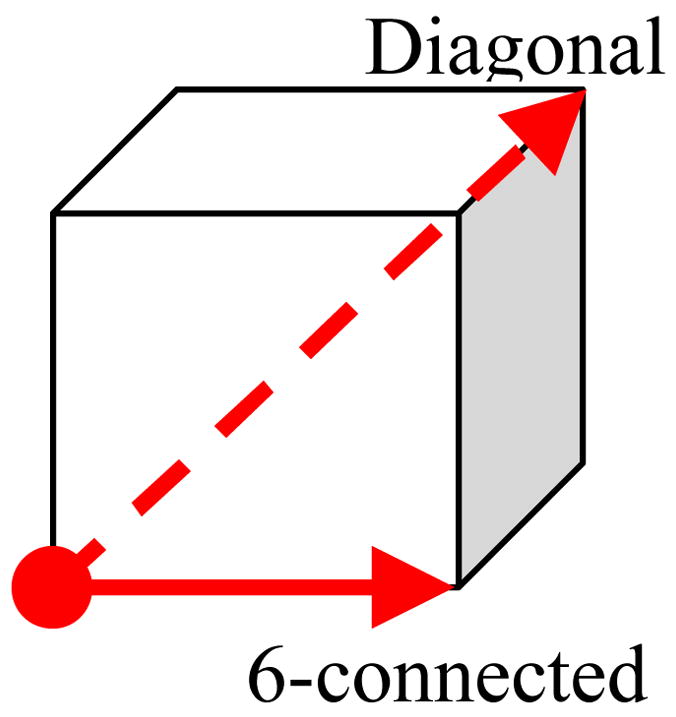
Voxel pairs on the geodesic path.

$$L_{GD}=\{\begin{array}{ll}\frac{\sqrt{3}+1}{2}·n_D·\delta \hfill & if{n}_D<\kappa \hfill \\ +\infty \hfill & \text{otherwise}\hfill \end{array}$$ (1)

where κ is a predefined constant used to stop the geodesic dilation for the case that the GD is extremely large, such as the stool and the polyp in Fig. 3(b). This upper bound is used to cover all the possibilities when applying the second criteria in Fig. 5, where the constant γ reflects the relative height of the SPs standing on the underlying major object for determining whether they are conceptually two objects or just parts of a single object.

2.2 The convex dilation (CD) strategy

Based on the polyp pathology in general [21], Wang et al. introduced the Harr transform-based fitting method to extract an elliptical inner border to satisfy the expectation that the inner border should be convex or flat. As mentioned in Section 1, the small contrast might fail the Harr transform-based edge finder, thus in this study, we introduce a convex dilation (CD) strategy to extract the VOI based on the conditional morphological dilation method [9]. For illustration purpose, we start from a brief introduction of the method [9]. An initial VOI is extracted by dilating for a few steps from a merged SP. The set of voxels {p_i} forming the initial VOI is denoted by V₀. Then the dilation process continues by a manner as depicted by V_n+1 = V_n ∪ N(V_n), where V_n represents the set of voxels at the step n of the dilation and N (V_n) represents the set of voxels in the soft tissues (excluding those in lumen) adjacent but not belonging to V_n, i.e.,

$$N(V_n)=\{p_i\mid p_i\in V_n^T,\mathit{and}{p}_i\notin V_n\},$$ (2)

where $V_n^T$ represents all the neighbors of V_n in the tissue region. Such iterative procedure would stop at a predefined maximum step n_M if a minimum growth rate could not be detected at any intermediate step n_m < n_M.

As mentioned in [14], the inner borders of the VOIs generated by the above dilation process would not be convex when the minimum growth rate could not be detected for sessile and flat lesions. In this paper, instead of using the Harr transformation-based edge finder [13, 14], we add an additional constraint to the aforementioned dilation process to address the problem, where N (V_n) is rewritten as

$$N(V_n)=\{p_i\mid p_i\in V_n^T,\mathit{and}{p}_i\notin V_n,\mathit{and}\zeta (p_i)>\alpha \}$$ (3)

where α is a constant threshold, and ζ (p_i) is defined as

$$\zeta (p_i)=\sum _{\mid p_j-p_i\mid <r}H(p_j)/\sum _{\mid p_j-p_i\mid <r}\left[1-H(p_j)\right]$$ (4)

where H (p_j) is a step function

$$H(p_j)=\{\begin{array}{ll}1\hfill & p_j\in V_n\hfill \\ 0\hfill & p_j\notin V_n\hfill \end{array}.$$ (5)

The underlying rationale of the above equations can be illustrated by a 2D case as shown in Fig. 7. The green area represents the current V_n. Considering pixel p₁ during the iteration at step n+1, the numerator and denominator at the right hand side of Eq. (4) actually measures the areas of the green and gray (including cyan) regions respectively in the red circle with the radius r. Therefore, ζ (p₁) measures the area ratio of the two regions. Straightforwardly, if such ratio is larger than 1, the green area is locally concave at pixel p₁. If it is less than or equal to 1 (i.e., the case at p₂), the green area is locally convex (at p₂). As a result, if the parameter α in Eq. (3) is set to be less than 1, the dilation process can make sure that the green area will grow into the gray area at concave pixels (such as p₁), but not at convex pixels (such as p₂). The dilation process (Eq. (3)) will stop automatically when ζ (p_i) is less than α at all pixels on the inner border. Therefore, the final dilated region will be convex everywhere.

Fig. 7.

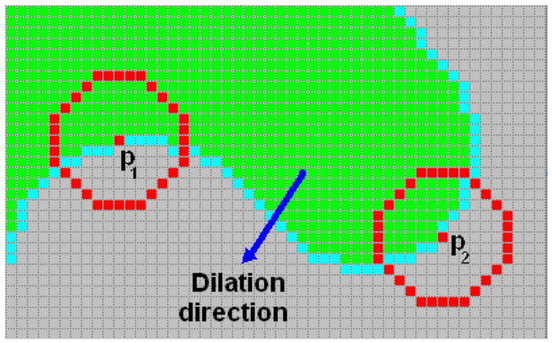
Illustration of the CD strategy in 2D case. The dilation process proceeds from the green area (pixels belong to V_n) to the gray area (pixels in tissue area outside V_n). Pixels in cyan represent the neighbors of V_n.

Two parameters are involved in the above equations, i.e., the constant threshold α, and the radius r. The first parameter determines the final convexity, which denotes how convex the final inner border would be with smaller value resulting more convex inner border. The second one reflects the degree of spatial locality, which depends on the size of the object under consideration. Straightforwardly, a larger radius should be used for a larger object. Theoretically, the curvedness represents the size of the object [24]. However, it is hard to get the meaningful curvedness on the colon wall [25]. Fortunately, the size of the object can be roughly reflected by the volume of the merged SP since a larger SP will be generated for a larger lesion candidate, hence proper value can be assigned to r accordingly (to be described in Section 3). Fig. 7 shows an example of VOI extraction for a 12 mm sessile polyp. From Fig. 7(a), it is difficult to visually figure out a meaningful inner border of the polyp. Fig. 7(b) shows the dilated initial V₀ and Fig. 7(c) is the result of the original method [9] with concave inner border. Fig. 7(d) shows the result by using the Harr transformation-based edge finder [14]. Obviously, the VOI is over-estimated, and the internal information of the VOI, e.g., the image intensity distribution, may be overwhelmed by the large amount of normal tissues. The CD strategy gives a more reasonable result as shown in Fig. 7(e) with a convex inner border as expected [21].

Fig. 7.

An experimental result of the CD strategy. (a) A 12mm sessile polyp in an axial slice, where the voxels in red indicate the SP. (b) The generated initial VOI V₀ in the slice (including the red and green area). (c) The result of the previous method in [9]. (d) The result of the previous method in [14], where the blue curve represents the inner border found by the Harr transformation-based edge finder. (e) The result of the presented CD strategy with r=9 and α =0.9.

III. Evaluation and results

3.1 CTC database

The presented two strategies were adapted to our previous CAD pipeline [14], as shown in Fig. 1, for evaluation purpose. The whole pipeline was applied to a CTC database including 50 patient studies. The patients were aged from 50 to 80 years. Each patient was scanned at both supine and prone positions, resulting in 100 CT scans by a multi-slice CT scanner (Light Speed Ultra, GE Medical Systems, Milwaukee, WI) in helical mode. The scanning protocol included mAs modulation in the range of 120–216 mA with kVp of 120–140 values. In the database, a total of 84 clinically significant polyps, sized in the range of 6–35 mm, were confirmed by both optical and virtual colonoscopies. In this evaluation, the supine and prone scans of each patient study were considered as different datasets, and the presented strategies were evaluated in terms of polyp detection and FP rate per dataset (or per CT scan). Therefore, there were 168 polyps in 100 CT scans in the CTC database.

3.2 Evaluation of the strategies

The initial suspicious patches (SPs) were detected by the use of the initial detector in our previous CAD pipeline [14]. The merge of the initial SPs were then performed by the above presented GDM strategy for an IPC. For each merged SP, its VOI was segmented by the presented CD strategy. Features were then extracted from the VOIs to differentiate TPs and FPs from all the IPCs. The differentiation task was accomplished by the use of SVM classifier. The gain by the presented GDM and CD strategies was shown by SVM outputs with comparison to our previous IPC detection methods.

3.2.1 The geodesic distance-based merging (GDM) strategy

In the GDM strategy, we extended L_m to be 20 mm in order to cover all possible polyp size. The predefined constant κ was determined for polyps as large as 40 mm (any polyp larger than 40 mm is expected to be detected easily without CAD help). The approximated GD should be larger than this key size κ. Therefore, κ was evaluated as $\lceil 80/[(\sqrt{3}+1)\delta ]\rceil +1$, where ⌈x⌉ denotes the largest integer which is larger than x.

In the evaluation, any case in which the polyp lobules (as shown in Fig. 2) were not merged was referred to as an unmerged polyp (UMP), i.e., a failure. On the other hand, any case in which neighboring polyps or non-polyp structures were merged with a polyp (as shown in Fig. 3) was referred to as a wrongly-merged polyp (WMP), another kind of failure. In the context of VOI extraction for polyp detection, we are only interested in the correct segmentation of true polyps, and we do not care about those unmerged or wrongly-merged non-polyp structures. Therefore, we will focus on the detection of the true polyps and the reduction of FPs. Under this condition, all the generated initial SPs by the initial detector in [14, 15] were input into the GDM module in Fig. 1 with various γ values, see Fig. 5. The incidences of UMPs and WMPs were calculated by per polyp. Multiple unmerged detections of one polyp were counted as one case of UMP. However, if n polyps were involved in a wrongly-merging scenario, n cases of WMP would be counted. For example, if one polyp was merged with a stool, it would be counted as one WMP. If two polyps were merged with a stool, it would be counted as two WMPs.

Fig. 8 plots the incidences of UMPs and WMPs according to different γ by experiments. The worst cases were 18 UMPs (with incidence of 10.7%) and 27 WMPs (with incidence of 16.1%) for the wide range value of γ. When γ is in the range [1.20, 1.24], there is no failure. For comparison purpose, we removed the second criteria in Fig. 5 and set L_m to be 12.5 mm, so that the above presented GDM strategy was reduced to exactly the same as that in the previous works [8, 9, 14, 15]. By repeating the same experiments, 15 UMPs and 29 WMPs were generated with the incidences to be 8.9% and 17.3% respectively.

Fig. 8.

The incidences of UMPs and WMPs according to the threshold γ.

3.2.2 The convex dilation strategy

As discussed in Section 2.2, the threshold α determines the final convexity of the inner border of a VOI. However, there is no theory or clinical reports about how convex the actual inner border of the polyp would be. In this study, we selected the value of α to be 0.9 by visually inspecting all the polyps in the CTC database. As for the other parameter, i.e., the radius r, its value can be roughly estimated according to the volume of each merged SP. By experiments, we found that r=5 was adequate for merged SPs with a volume smaller than 40 mm³, which indicates a polyp of intermediate size (6–9 mm), while a larger value r=9 worked well for larger polyps.

To evaluate the CD strategy (of extracting the VOI of each IPC from the corresponding merged SPs), two texture features, the mean and variance of the CT intensities inside the VOI, were utilized since their outcomes would reflect the performance of the VOI extraction strategy. For comparison purpose, two previous methods were implemented: (1) the conditional morphological dilation method [9] and (2) the Harr transform-based inner border extraction method [14]. The 100 CT scans were randomly split into two equal-sized groups, and the feature vectors of the IPCs in the two groups formed the training and testing sets, respectively, for SVM classification [14]. The performances of the three VOI extracting procedures (the presented strategy and the two previous methods) were measured by the free-response receiver operating characteristics (fROC) curves, where the vertical axis reflects the by-polyp sensitivity and the horizontal axis represents the FP rate per dataset. The grouping process of the training and testing sets was repeated 20 times randomly for the three methods and the average of the 20 trials was used to overcome the bias in the datasets.

Fig. 9 shows the fROC curves of the three methods. The rectangle on each operation point represents the confidence intervals for the sensitivity and FP rate with 95% confidence level. Table 1 lists the performance of the three methods at their highest detection sensitivities, as indicated by the black dots in Fig. 9.

Fig. 9.

The fROC curves of the testing procedures. The three curves depict the performance of the three VOI extraction methods using the two features. The transparent rectangle at each point on the three curves denotes the confidence intervals (95% confidence level) for the sensitivity and FP rate.

Table 1.

Performance of the three methods.

	Method [9]	Method [14]	CD strategy
Sensitivity	0.91 (0.81–0.95)	0.89 (0.80–0.94)	0.96 (0.88–1.00)
FP rate	5.02 (4.42–5.42)	5.56 (4.98–6.00)	4.52 (4.22–4.72)

The lengths of the confidence intervals (the height and width of the rectangle) at each operation point in Fig. 9 were investigated with their mean and standard deviation (std), as tabulated in Table 2.

Table 2.

Confidence interval comparison.

		Method [9]	Method [14]	The CD strategy
Sensitivity	mean	0.1040	0.0927	0.0720
	std	0.0325	0.0294	0.0224
FP rate	mean	0.2493	0.2827	0.1453
	std	0.2224	0.2758	0.1227

IV. Discussion and conclusion

It can be seen in Fig. 8 that the incidence of UMPs decreases but that of WMPs increases with the threshold γ. This is because γ denotes the ratio of the GD and ED between any two SPs and indicates how high the SPs stand on the colon wall. According to the flowchart in Fig. 5, a smaller γ discourages the merging process even though the SPs stand low on the colon wall, and leads to more cases of unmerged lobules of a polyp. On the contrary, a larger γ encourages the merging processes although the SPs stand high on the bladder wall, and leads to higher incidence of WMPs. In Fig. 8, the zero-incidence of both UMPs and WMPs was achieved if γ was set to be about 1.22. However, the previous ED-based merging method with any L_m would generate undesirable merging cases, e.g. 15 UMPs and 29 WMPs were created when L_m = 12.5 mm in the experiments and more WMPs/UMPs would be expected with larger/smaller L_m.

The fROC curves in Fig. 9 show the performance after 20 runs of the classifier based on the VOIs generated with the three different methods. The confidence intervals of the two curves of the methods in [9] and [14] have significant overlaps indicating that the two VOI extraction methods perform comparably. However, the curve of the CD strategy in this paper generally stays upon both of the other two curves, and so does the confidence interval at each operation point, which is fairly obvious in the FP rate range of 0.4 to 4. Generally, we can claim that the CD strategy for VOI extraction outperforms the other two methods.

As listed in Table 1, at the highest detection sensitivities, i.e., 0.91 of the method in [9], 0.89 of the method in [14] and 0.96 of the CD strategy, the corresponding FP rates are 5.02, 5.56 and 4.52 respectively. The features from the VOIs generated by the CD strategy perform the best by yielding the highest by-polyp sensitivity at the lowest FP rate.

Table 2 tabulates the mean and standard deviation of the confidence intervals of the sensitivity and FP rate at each operation point of the three fROC curves. The CD strategy yields smallest values of all the statistics, suggesting that the features from the generated VOIs by the CD strategy perform more robust and consistent in distinguishing TPs and FPs in the 20 runs of the classification process mentioned in Section 3.2.2.

It is noted that the method [9] performs slightly better than the method [14] according to Fig. 9, Table 1 and Table 2. This can be explained as follows. The very low image contrast between polyp and normal tissue renders a challenge for the Harr transform-based edge finder, and the generated VOIs may include more normal tissue voxels (see Fig. 7(d)). These redundant voxels may dilute the characterizing capability of the two features, i.e., the mean and variance of the CT intensities, extracted from the VOI.

The evaluation was based on a CTC database including 100 scans with 84 polyps sized in the range of 6–35 mm. We argue that the number of polyps is large enough for the evaluation purpose. However, as mentioned in Section 3.2, there are several parameters dependent on the size of polyps, such as the merging distance L_m, the constant κ used in the GDM strategy and radius r used in the CD strategy. Although the values of these parameters have worked pretty well for our current database, they would need to be investigated by using more polyps larger than 35 mm and smaller than 6 mm.

In conclusion, compared to the ED-based merging method [14, 15], the GDM strategy can effectively reduce the incidence of the undesirable merging cases, like UMPs and WMPs, and even achieve zero-incidence at certain circumstance. The CD strategy can ensure the convexity of the inner border of the IPCs to meet the expectation [21]. By using two simple, while VOI-related, features, the experimental results showed that the resulted VOIs outperform those with concave inner borders [9] or generated by the intensity contrast-based edge finder [14]. As our future work, other features rooting from the VOI will be utilized to validate the improvement of the presented strategies with a larger polyp database.

References

- 1.American Cancer Society. Cancer Facts & Figures 2008. Atlanta: American Cancer Society; 2008. [Google Scholar]
- 2.Eddy D. Screening for Colorectal Cancer. Annals of Internal Medicine. 1990;113:373–384. doi: 10.7326/0003-4819-113-5-373. [DOI] [PubMed] [Google Scholar]
- 3.Pickhardt P, Choi J, Hwang I, Butler J, Puckett M, Hildebrandt H, Wong R, Nugent P, Mysliwiec P, Schindler W. Computed tomographic virtual colonoscopy to screen for colorectal neoplasia in asymptomatic adults. New England Journal of Medicine. 2003;349(23):2191–2200. doi: 10.1056/NEJMoa031618. [DOI] [PubMed] [Google Scholar]
- 4.Summers R, Yao J, Pickhardt P, Franaszek M, Bitter I, Brickman D, Krishna V, Choi R. Computed tomographic virtual colonoscopy computer-aided polyp detection in a screening population. Gastroenterology. 2005;129:1832–1844. doi: 10.1053/j.gastro.2005.08.054. [DOI] [PMC free article] [PubMed] [Google Scholar]
- 5.Bielen D, Kiss G. Computer-aided detection for CT colonography: update 2007. Abdominal Imaging. 2007;32:571–581. doi: 10.1007/s00261-007-9293-2. [DOI] [PubMed] [Google Scholar]
- 6.Summers RM, Beaulieu CF, Pusanik LM, Malley JD, Jeffrey RB, Glazer DI, Napel S. Automated polyp detector for CT colonography: feasibility study. Radiology. 2000;216:284–290. doi: 10.1148/radiology.216.1.r00jl43284. [DOI] [PubMed] [Google Scholar]
- 7.Yao J, Miller M, Franaszek M, Summers RM. Colonic polyp segmentation in CT colonography-based on fuzzy clustering and deformable model. IEEE Transactions on Medical Imaging. 2004;23(11):1344–1352. doi: 10.1109/TMI.2004.826941. [DOI] [PubMed] [Google Scholar]
- 8.Yoshida H, Nappi J. Three-dimensional computer-aided diagnosis scheme for detection of colonic polyps. IEEE Transactions on Medical Imaging. 2001;20(12):1261–1274. doi: 10.1109/42.974921. [DOI] [PubMed] [Google Scholar]
- 9.Nappi J, Yoshida H. Feature-guided analysis for reduction of false positives in CAD of polyps for computed tomographic colonography. Medical Physics. 2003;30(7):1592–1601. doi: 10.1118/1.1576393. [DOI] [PubMed] [Google Scholar]
- 10.Suzuki K, Yoshida H, Nappi J, Armato SG, III, Dachman AH. Mixture of expert 3D massive-training ANNs for reduction of multiple types of false positives in CAD for detection of polyps in CT colonography. Medical Physics. 2008;35(2):694–703. doi: 10.1118/1.2829870. [DOI] [PubMed] [Google Scholar]
- 11.Acar B, Beaulieu CF, Gokturk SB, Tomasi C, Paik DS, Jeffrey B, Yee J, Napel S. Edge displacement field-based classification for improved detection of polyps in CT colonography. IEEE Transactions on Medical Imaging. 2002;21(12):1461–1467. doi: 10.1109/TMI.2002.806405. [DOI] [PubMed] [Google Scholar]
- 12.Paik D, Beaulieu C, Rubin G, Acar B, Jeffrey B, Yee J, Dey J, Napel S. Surface normal overlap: a computer-aided detection algorithm with application to colonic polyps and lung nodules in helical CT. IEEE Transactions on Medical Imaging. 2004;23(6):661–675. doi: 10.1109/tmi.2004.826362. [DOI] [PubMed] [Google Scholar]
- 13.Wang Z, Liang Z, Li L, Li X, Anderson J, Harrington D. Reduction of false positives by internal features for polyp detection in CT-based virtual colonoscopy. Medical Physics. 2005;32(12):3602–3616. doi: 10.1118/1.2122447. [DOI] [PMC free article] [PubMed] [Google Scholar]
- 14.Zhu H, Duan C, Pickhardt P, Wang S, Liang Z. Computer-aided detection of colonic polyps with level set-based adaptive convolution in volumetric mucosa to advance CT colonography toward a screening modality. Cancer Management and Research. 2009;1(1):1–13. doi: 10.2147/cmar.s4546. [DOI] [PMC free article] [PubMed] [Google Scholar]
- 15.Wang S, Zhu H, Lu H, Liang Z. Volume-based feature analysis of mucosa for automatic initial polyp detection in virtual colonoscopy. International Journal of Computer Assisted Radiology and Surgery. 2008;3(1–2):131–142. doi: 10.1007/s11548-008-0215-8. [DOI] [PMC free article] [PubMed] [Google Scholar]
- 16.Bhotika R, Mendonca PR, Sirohey SA, Turner WD, Lee YL, McCoy JM, Brown RE, Miller JV. Part-based local shape models for colon polyp detection. Med Image Comput Comput Assist Interv Int Conf Med Image Comput Comput Assist Interv. 9(Pt 2):479–486. doi: 10.1007/11866763_59. [DOI] [PubMed] [Google Scholar]
- 17.Kiss G, Cleynenbreugel J, Thomeer M, Suetens P, Marchal G. Computer-aided diagnosis in virtual colonography via combination of surface normal and sphere fitting methods. European Radiology. 2002;12(1):77–81. doi: 10.1007/s003300101040. [DOI] [PubMed] [Google Scholar]
- 18.Chowdhury T, Whelan P, Ghita O. The use of 3D surface fitting for robust polyp detection and classification in CT colonography. Computerized Medical Imaging and Graphics. 2006;30(8):427–436. doi: 10.1016/j.compmedimag.2006.06.004. [DOI] [PubMed] [Google Scholar]
- 19.Jerebko A, Teerlink S, Franaszek M, Summers RM. Polyp segmentation method for CT colonography computer-aided detection. SPIE Medical Imaging; Feb. 16; San Diego, CA. 2003. pp. 359–369. [Google Scholar]
- 20.van Wijk C, van Ravesteijn VF, Vos FM, Truyen R, de Vries AH, Stoker J, van Vliet LJ. Detection of protrusions in curved folded surfaces applied to automated polyp detection in CT colonography. Med Image Comput Comput Assist Interv Int Conf Med Image Comput Comput Assist Interv. 2006;9(Pt 2):471–478. doi: 10.1007/11866763_58. [DOI] [PubMed] [Google Scholar]
- 21.Haggitt R, Glotzbach R, Soffer E, Wruble L. Prognostic factors in colorectal carcinomas arising from adenomas: Implications from lesions removed by endoscopic polypectomy. Gastroenterology. 1985;89(1):328–336. doi: 10.1016/0016-5085(85)90333-6. [DOI] [PubMed] [Google Scholar]
- 22.Kimmel R, Sethian J. Computing geodesic paths on manifolds. Proceedings of National Academy of Sciences. 1998;95:8431–8435. doi: 10.1073/pnas.95.15.8431. [DOI] [PMC free article] [PubMed] [Google Scholar]
- 23.Dijkstra EW. A Note on Two Problems in Connection with Graphs. Numerische Math. 1959;1:269–271. [Google Scholar]
- 24.Dorai C, Jain AK. COSMOS A representation scheme for 3D free-form objects. IEEE Transaction of Pattern Analysis and Machine Intelligence. 1997;19:1115–1130. [Google Scholar]
- 25.Nappi J, Dachman A, MacEneaney P, Yoshida H. Computer-aided detection of polyps in CT colonography: evaluation of volumetric features in differentiating polyps from false positives. International Congress Series. 2001;1230:676–681. [Google Scholar]