A Novel Cell Segmentation Method and Cell Phase Identification Using Markov Model

Abstract

Optical microscopy is becoming an important technique in drug discovery and life science research. The approaches used to analyze optical microscopy images are generally classified into two categories: automatic and manual approaches. However, the existing automatic systems are rather limited in dealing with large volume of time-lapse microscopy images because of the complexity of cell behaviors and morphological variance. On the other hand, manual approaches are very time-consuming. In this paper, we propose an effective automated, quantitative analysis system that can be used to segment, track, and quantize cell cycle behaviors of a large population of cells nuclei effectively and efficiently. We use adaptive thresholding and watershed algorithm for cell nuclei segmentation followed by a fragment merging method that combines two scoring models based on trend and no trend features. Using the context information of time-lapse data, the phases of cell nuclei are identified accurately via a Markov model. Experimental results show that the proposed system is effective for nuclei segmentation and phase identification.

I. Introduction

Time-lapse fluorescence microscopy, as an important technique for studying the dynamic cell cycle behaviors of a large population of cells, is attracting more and more attention [1], [2]. Its significance surges mainly because of its potential in achieving new and high-throughput way to conduct drug discovery and quantitative cellular studies [3]. However, it is difficult to process and analyze large volumes of images generated by time-lapse microscopy because the increasing quantity and complexity of imaged data from dynamic microscopy renders the manual analysis unreasonably time-consuming. In addition, to the best of our knowledge, currently there is no effective automated system that can meet this requirement in real tasks. Thus, the lack of an automated system that can segment, track, and classify large volumes of cellular image data automatically is becoming the bottleneck of studying the cell cycle process in a systematic, quantitative, and large-scale manner.

Our goal is to develop an automated analysis system to segment, track, and quantize the cell cycle behaviors of a population of cells. Fig. 1 shows the flowchart of the proposed system. The system consists of four major components: image preprocessing, nuclei segmentation, nuclei tracking, and cell phase identification. Although a lot of previous work has focused on some subproblems such as segmentation and cell phase identification [2], [4], [5], it is difficult to consider the problems from a systematic view due to error propagation. On the other hand, from a systematic view, there is additional information available for improving the performance of the whole system.

Fig. 1.

Flowchart of the proposed system.

Four steps are involved in the image preprocessing component: image enhancement [6], adaptive thresholding [7], morphological filtering [8], and distance transformation [9]. In the segmentation, we merge the oversegmented nuclei via a hybrid merging algorithm after the watershed segmentation [10]. In the hybrid merging method, the selected features are classified into two classes: features with trend and features with no trend. Then, the two classes of features are used separately to compute two scores of fragments. The two scores are combined together to guide the final merging decision. We do tracking using the nearest neighbor matching method. Cell phase identification is a traditional classification problem in the area of data mining. Many classifiers have been tried in previous work. Their work shows that K-nearest neighbor (K-NN) can achieve very good performance for all cell phase identification [2]. Nevertheless, in our experiments, the accuracy was only about 50% for prophase cell nuclei by using K-NN. Herein, we propose to improve the classification performance using the context information. A continuous Markov model [11], [12] is used for phase identification to achieve higher accuracy.

The rest of this paper is organized as follows. In Section II, we present the image preprocessing, nuclei segmentation, and tracking. The statistical Gaussian mixture Markov model is proposed for the context-based cell phase identification in Section III. We show the experimental results in Section IV, and the conclusion remarks are presented in Section V.

II. Nuclei Segmentation and Tracking Procedure

A. Image Preprocessing

Digital images usually require preprocessing to remove noise, undesirable features, and correct illumination artifacts. The preprocessing consists of four steps: contrast enhancement, adaptive threshold, morphological filtering, and distance transformation. To enhance the intensity contrast, the top hat and bottom hat filters (radius = 15 pixels) are adopted [6]. It is well known that a global threshold cannot generate good binary image results because of the variation of the background and the existence of dark nuclei, so the adaptive threshold method proposed in [13] is employed. We compute the threshold of each pixel as follows:

$$T(x,y)=\underset{\mid i-x\mid <=w,\mid j-y\mid <=h}{\text{mean}}\{I(i,j)\}$$ (1)

where w and h are the width and height of the local window. In this study, we choose the local window with width w = 30 pixels and height h = 30 pixels. We set the size of the local window empirically such that the size of the window is larger than the size of the largest cell. The small fragments of noises can be eliminated by the morphological opening operation (radius = 5 pixels), and the holes on the nuclei can be filled by using the morphological closing operation (radius =5 pixels) [8]. Finally, the distance transformation [9] is applied on the binary image.

B. Segmentation and Fragments Merging

Nucleus segmentation is an essential part in the proposed system because the segmentation results directly affect the accuracy of the following tracking and phase identification. Though the adaptive threshold can segment all the cell nuclei from background effectively, it cannot separate the touching nuclei. To solve this problem, we apply watershed algorithm on the distance image to separate the cell clusters [10]. However, the watershed segmentation algorithm generally results in oversegmentation, as seen in Fig. 2(b). To reduce the oversegmentation, we propose a hybrid fragments merging approach that combines the compactness score and probability distribution function (PDF) score. In the following, we present the details of the hybrid fragments merging method.

Fig. 2.

Example segmentation results. (a) Original image. (b) Result of watershed algorithm. (c) Result after the hybrid merging algorithm.

1) PDF Merging and Compactness Merging

To reduce the oversegmentation, a feature-based merging technique is employed. Similar to previous work in objects merging [2], [14], we transformed all the fragments (segmented cell nuclei) into an eight-dimension feature vector space: maximum intensity, minimum intensity, standard derivation of intensity, average intensity, length of major axis, length of minor axis, perimeter, and compactness (perimeter²/4π × area). We select these eight features using the a.k.a. discriminant analysis.

Generally, the feature-based merging techniques can be classified into two classes: one is rule-based method such as size-based merging algorithm [15], [16] and the other is statistical-based approach, i.e., PDF merging algorithm [14]. The-rule based merging methods use one feature (rule), e.g., size, integrated intensity, as a score of each fragment to evaluate the probability of the fragment being a well-segmented cell nucleus. For example, the experiment in [15] assumed that the larger the fragment, the higher the probability of being a well-segmented cell. The authors in [16] assumed that the fragment has high probability of being a well-segmented nucleus if its integrated pixel intensity is high.

Compared with the rule-based merging method, PDF merging combines multiple features together to generate a measure score, and the probabilities of fragments belonging to well-segmented nuclei are computed based on the training dataset in the selected feature space. Two fragments are merged if the integrated fragment gives a higher probability. Usually, the PDF score (S̃_pi) of fragment x_i could be calculated using Gaussian distribution. The probability of the fragment being a well-segmented cell becomes higher as the score becomes larger. For the PDF merging method, one limitation is that its performance closely depends on the training data. Except the difficulty of automatic collection of training data, it is not always true that a real cell should be close to the training data in some specific features. As an example, thinking a measure R = (perimeter of convex hull)/perimeter, it is obvious that we should assume that if a fragment i is a well-segmented cell nucleus, R should be close to 1. However, the R feature of training data are always larger than 1. Then, mistakes are introduced by PDF merging algorithm. For instance, suppose the mean value of the training data in feature R is 1.2, the value of R of two fragments are 1.05 and 1.15, respectively: which one has a larger probability of being a well-segmented cell nucleus? If we must choose one to merge, the traditional PDF merging will choose the first one and intuitively we should choose the second one to merge, because the R feature of 1.05 is close to 1.

Motivated by the aforementioned fact, we classify the eight selected features into two classes. One class consists of seven features with no trend: maximum intensity, minimum intensity, average intensity, standard derivation of intensity, length of major axis, length of minor axis, and perimeter. We call them features with no trend because we do not know the probability of a fragment being a well-segmented cell nuclei from the values of these features. We use the PDF merging method on these features with no trend. The principal component analysis (PCA) is used to reduce the seven-dimension feature space into two-dimension space. The selection of training data can be automatically conducted by finding all the cell nuclei that have no adjacent neighbors for the PDF merging method. On the other hand, we call the compactness as the feature with trend. The merging decision can be made directly based on the following rule: one fragment is more like being a well-segmented nucleus if its compactness value (S̃_Ri) is smaller because the fragment with more round shape has smaller compactness value. The merging rule is that we merge fragments i and j if S̃_Rij < S̃_Ri and S̃_Rij < S̃_Rj, where S̃_Rij is the compactness score of a fragment that consists of fragment i and fragment j. We call this as compactness merging.

2) Hybrid Merging Algorithm

In the following, we propose to integrate two measure scores together to direct the final merging decision. We name it hybrid merging. We first transform S̃_Ri into [0, [1] as S_Ri = S̃_Ri/(S̃_Ri + S̃_Rj + S̃_Rij). In addition, S̃_Pi is normalized to [0, [1] as S_Pi = S̃_Pi/(S̃_Pi + S̃_Pj + S̃_Pij), and then, the combined merging score of fragment i, j and the merged fragment i and j could be computed as

$$\{\begin{array}{l}{S}_i=w_1{S}_{Ri}+w_2{S}_{Pi}\\ S_j=w_1{S}_{Rj}+w_2{S}_{Pj}\\ S_{ij}=w_1{S}_{\mathit{Rij}}+w_2{S}_{\mathit{Pij}}\end{array}$$ (2)

where w₁ and w₂ are the weights of compactness score and PDF score that satisfy w₁ + w₂ = 1, w₁ > 0, and w₂ > 0, and S_ij denotes the combined score of a new fragment that consists of fragment i and fragment j. We merge cell i and cell j if and only if S_ij > S_i and S_ij > S_j. In other words, if the merged fragment looks more like being a well-segmented cell nucleus than the two fragments, we merge them; otherwise, we will not merge them. Fig. 2(c) provides a representative merging result. To estimate the two weights, we first collected two testing datasets: one set consists of fragments that are oversegmented and should be merged, and the other set consists of fragments that are well segmented and should not be merged. Then, we chose the values of w₁ and w₂ that best separate the two testing datasets from 100 discrete possible pairs:{(0.01, 0.99), (0.02, 0.98), …, (0.99, 0.01)}. The chosen values of w₁ and w₂ are 0.87 and 0.13.

3) Nuclei Tracking

Cell nuclei tracking is an essential part for quantitative study of cell cycle behaviors, including cell migration, phase progress, division, and death. In this study, we employ an NN-based tracking method proposed in [2]. First, we define a distance- and size-based matching similarity measure, and then, we generate the distance matrix Dis = {dis_ij} to store all the distances between nuclei in frame t and their possible counterparts in frame t + 1, i.e., dis_ij (t) is the distance between x_i (t) and x_j (t + 1). After that we do the cell matching as follows: to cell x_i (t), we scan the adjacent matrix to find all possible candidates being its successive cells and the candidates at frame t + 1 are added one by one according to their distance to the nucleus at time t. A nucleus with the smallest distance is added first and the largest one last. Each time when a nucleus is added, the sum size is compared with the size of x_i (t). If the sum size is more than 10% larger than the size of x_i (t), we stop and discard the new added one. We choose 10% as the threshold since the area of x_i (t) cannot increase more than 10% in the next frame in accordance with our experience in this study. Some over- and undersegmentation can also be corrected by using context information. For details, refer to [2]. In this study, we can detect four cell phases: interphase, prophase, metaphase, and anaphase, as seen in Fig. 3. In mitosis, the cells experience the prophase, metaphase, and anaphase. At the end of metaphase, one nucleus is divided into two parts. In the tracking, we can only detect the cell migration, division, and the death points. However, the cell phase information cannot be obtained in the tracking step and the segmentation errors may influence the tracking results. To better quantify the cell cycle activities, we further identify the cell phases using the Markov model.

Fig. 3.

Four cell phases. (a) Interphase. (b) Prophase. (c) Metaphase. (d) Anaphase.

III. Cell Phase Identification by Markov Model

The performance of statistical-method-based cell phase identification approaches closely depends on the selected features and the design of classifiers. Additionally, there are some cases where the pure feature-based approaches do not work. For example, it is difficult to identify the phases of the overlapped cell nuclei because the features extracted from these overlapped ones are highly noised by each other. To improve the cell identification accuracy, we utilize both the features and the context information in Markov model [11].

A. Markov Model

In this study, we employ Markov model to identify the cell phases based on the context information. The model is the “left–right” model shown in Fig. 4. The transition from phase 1 (interphase) to phase 3 (metaphase) in Fig. 4 could happen sometimes because the dwelling time of phase 2 (prophase) could be very short and sampling period could be longer than that. The occurrence of the first phase in the sequence is characterized by the initial probability of the sequence, and the occurrence of the other phase, which was given by the occurrence of its previous phase, is characterized by the transition probability. Given a set of training cell sequences, the initial and the transition probabilities are calculated. In addition, we model the distribution of each phase by R Gaussian mixtures. We optimize these Gaussian mixtures by expectation–maximization (EM) algorithm [12].

Fig. 4.

Diagram of the four states left–right Markov model. The four states are as follows. (1) Interphase. (2) Prophase. (3) Metaphase. (4) Anaphase. Each state is modeled as a Gaussian mixture model with two mixtures.

Mathematically, suppose a set of N training sequences (χ₁, χ₂, …, χ_N) is given and the phases of all the cell nuclei in these sequences are known. Each sequence is a cell nucleus in T_l different frames ${\chi }_l=(X_1^l,X_2^l,\dots ,X_{T_l}^l)$, l = 1, 2, …, N, where each cell nucleus is denoted by a p-dimensional feature vector $X_t^l=(x_{t1}^l,X_{t2}^l,\dots ,X_{tp}^l)$, t = 1, 2, …, T. In this study, $X_t^l$ is a 2-D feature vector obtained by applying the PCA to the seven features, as seen in Section II-B1. On the other hand, let S = {s₁, s₂, …, s_M} be the set of M states in Markov chain, and we also consider the N training sequences as a group of T_l length random variables ${\mathrm{\Theta }}_l=\{{\theta }_1^l,{\theta }_2^l,\dots ,{\theta }_{T_l}^l\}$. The sample space of these variables is S. For simplification, here we assume that the state of an object at time t depends only on its state at time t − 1. So we can get the conditional probabilities $Pr({\theta }_t^l=s_j\mid {\theta }_{t-1}^l=s_i,{\theta }_{t-2}^l=s_{i2},\dots ,{\theta }_1^l=s_{i1})=Pr({\theta }_t^l=s_j\mid {\theta }_{t-1}^l=s_i)$, i, j = 1, 2, …, M. We develop a model to represent the phase sequences found in a given set of cells. To the lth training sequence, define the following parameters: $\mathrm{\Pi }\triangleq [{\pi }_i],A\triangleq [a_{ij}]$, where ${\pi }_i=Pr({\theta }_1^l=s_i)$ and $a_{ij}=Pr({\theta }_t^l=s_j\mid {\theta }_{t-1}^l=s_i)$, l = 1, 2, …, N, i, j = 1, 2, …, M, t = 2, …, T, Π is called the initial probability, and A is called the transition probability matrix. They must satisfy the constrains ${\sum }_{i=1}^M{\pi }_i=1,{\sum }_{j=1}^M{a}_{ij}=1$, i, j = 1, 2, …, M. To the training sequence set, we initialize Π and A by

$${\pi }_i=\frac{n_i}{{\sum }_{k=1}^M{n}_k}\text{and}{a}_{ij}=\frac{n_{ij}}{{\sum }_{k=1}^M{n}_{ik}}$$ (3)

where n_i and n_ij are the number of occurrences of ${\theta }_1^l=s_i$ and ${\theta }_t^l=s_j$ when ${\theta }_{t-1}^l=s_i$ in the sequence set.

To our Markov model, we model each phase using R Gaussian mixtures ϕ(X, μ_kr, Σ_kr), k = 1, 2, …, M, r = 1, 2, …, R, where μ_kr and Σ_kr are the means and covariance matrices of Gaussian mixtures. In this study, we set M = 4 and R = 2. In addition, we have a group of coefficients c_kr to weight the Gaussian mixtures of each state. The Gaussian mixtures of each phase can be initialized by fuzzy c-means [17], and eventually, μ_kr and Σ_kr are initialized based on the results of fuzzy c-means. As a conclusion, our proposed continuous Markov model can be described by a group of parameters

$$\mathrm{\Lambda }=\{\mathrm{\Pi },A,{\mu }_{kr},{\mathrm{\sum }}_{kr},c_{kr},k=1,2,3,4;r=1,2\}.$$ (4)

After initialization, all the parameters are optimized by EM algorithm iteratively. The detailed equations are given in [12].

1) Cell Phase Classification

According to Gaussian mixture model [12], the probability of a cell X_t belonging to phase s_m, i.e., θ_t = s_m, should depend only on X_t and X_{t − 1}. Thus, the probabilities we need for the categorization of cells could be denoted as p(θ_t = s_m |X_t, X _{t − 1}). Based on the Bayesian formula, we can rewrite them as

$$\begin{array}{l}p({\theta }_t=s_m\mid X_t,X_{t-1})\\ \propto \sum _{i=1}^M{\pi }_i{a}_{im}p(X_t,X_{t-1}\mid {\theta }_t=s_m,{\theta }_{t-1}=s_i)\end{array}$$ (5)

where m = 1, …, M and p(X_t, X_{t − 1} |θ_t = s_j, θ_{t − 1} = s_i) means that given θ_t = s_j and θ_{t − 1} = s_i, the probability of Gaussian mixtures ϕ(X, μ_jr, Σ_jr) and ϕ(X, μ_ir, Σ_ir) can generate vectors X_t and X_{t − 1}. Finally, we classify cell X_t to phase s_m^*, i.e., θ_t = s_m^* if and only if

$$s_{m^{\ast }}=\underset{m=1,2,\dots ,M}{argmax}\{p({\theta }_t=s_m\mid X_t,X_{t-1})\}.$$ (6)

Although the Markov model tries to model the context information of the nuclei sequences, it does not mean that the classification results perfectly follow biological phenomena because of noisy data. From the biological point of view, the anaphase cell nuclei in a sequence cannot last more than three frames (the imaging time interval is 15 min in this study). In addition, no cell nucleus can jump from interphase or prophase to anaphase directly. We apply this rule after the classifier to improve the classification performance. We call it Markov model with rule in this paper. In this study, we also use the biological rules described in [2]: 1) cell cycle progress forward rule: cell cycle progress can only go forward and 2) cell phase timing rule: the time period that a cell stays in a phase cannot change dramatically.

IV. Experiments

The cells used in this paper are HeLa cell line. We acquired cellular images per 15 min with a time-lapse fluorescence microscopy. Each image is of 672 × 512 pixels. Our experiments were conducted on the data over a period of two days. In other words, each cellular image sequence consists of 192 frames. We implemented the software named DCellIQ on both Matlab platform and windows-based C++ platform, respectively. For an image with approximately 300 nuclei, the segmentation time by DCellIQ was about 1.6 s on a Pentium IV 2.4-GHz computer. Note that less than 1 s was required to track a trace. An exception is that nuclei that left or disappeared in the field of view during the whole sequence were ignored.

A. Results of Segmentation

To test the segmentation algorithm, 20 images were chosen from the 192 images involved. The frames used are frame 1, frame 20, frame 40, frame 60, frame 80, frame 100, frame 120, frame 140, frame 160, frame 180, and others are chosen randomly by computer. This generates a test set consisting of 5596 nuclei. To show the effectiveness of our proposed algorithm, four approaches are tested:

1. watershed, simple watershed algorithm without fragments merging;

2. PDF, watershed algorithm with all feature used PDF merging;

3. hybrid, watershed algorithm with the hybrid merging algorithm proposed in this paper;

4. hybrid + context, the hybrid merging with context-based correction proposed in [2].

We selected the training set for PDF merging by the approach introduced in Section II-B1. Table I shows the detailed segmentation results. The ground truth is given by manual analysis done as follows: we run the algorithm and then a biologist verified whether or not they were segmented correctly. It can be seen that without fragment merging, the watershed algorithm can only correctly segment 90.35% of the nuclei. The popularly used PDF merging can correctly segment 95.10% of the cell nuclei. On the other hand, our proposed hybrid merging algorithm can correctly segment 97.41% of the nuclei. In addition, the accuracy could be improved to 98.12% after the context-based correction.

TABLE I.

Segmentation Results Comparison

	Tested	Correct Segmented	Over Segmented	Under Segmented
Watershed	5596	5056 (90.35%)	482 (8.61%)	58 (1.03%)
PDF	5596	5322 (95.10%)	207 (3.7%)	87 (1.55%)
Hybrid	5596	5451 (97.41%)	102 (1.82%)	43 (0.77%)
Hybrid+ Context	5596	5508 (98.43%)	64 (1.14%)	24 (0.43%)

B. Results of Cell Phase Identification

We selected 50 full-length cell tracks as training data and all these 192 × 50 = 9600 cell nuclei were labeled manually. Among the 9600 cell nuclei, 9154 of them were in interphase, 58 of them were in prophase, 267 of them were in metaphase, and 121 of them were in anaphase. We assumed that cell nuclei in the same sequence should have similar intensities; thus, we normalized the features of cell nuclei trace by trace before we classified them using Markov model. Fig. 5 shows the 2-D visualization of all the 9600 training cell nuclei in the reduced feature space using PCA. It is obvious that no linear classifier worked well based on these kinds of data. We selected 150 sequences from three datasets (50 sequences per dataset) as the test data to test the performance of continuous Gaussian mixture Markov model for phase identification. Two approaches were used as baseline algorithms: one was maximum likelihood (ML) classifier and the other was K-NN (K = 5, 7) classifier. Table II shows the results of our proposed approach, ML classifier, and K-NN, respectively.

Fig. 5.

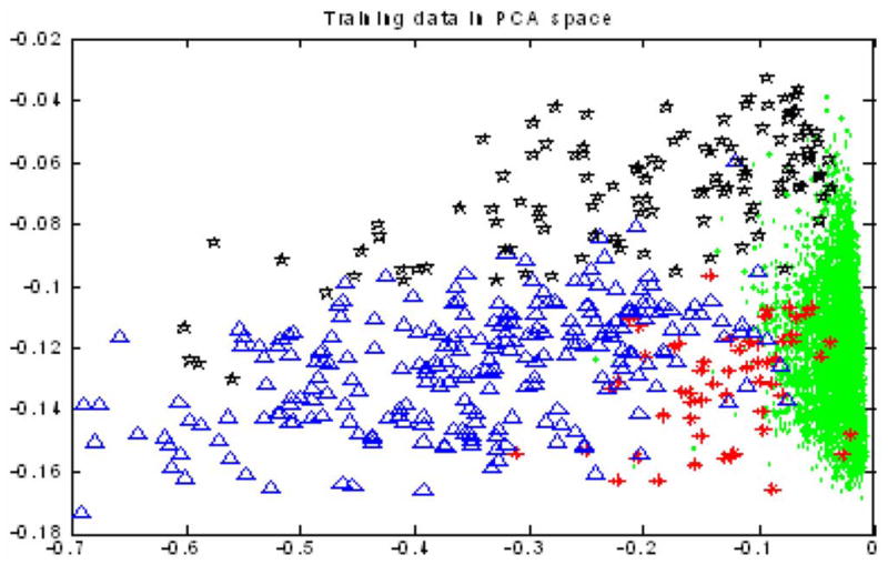
2-D visualization of all the 9600 nuclei in the training dataset. Green spots—interphase; red stars—prophase; blue triangles—metaphase; and black pentacles—anaphase.

TABLE II.

Cell Phase Identification Results: Internumber of Interphase, Pronumber of Prophase, Metanumber of Metaphase, Ananumber of Anaphase

		Inter	Pro	Meta	Ana	Total	Accuracy
ML	Inter	25434	1161	28	731	27354	92.98%
	Pro	35	113	29	4	181	62.43%
	Meta	68	30	633	172	903	70.10%
	Ana	34	5	47	276	362	76.24%
Markov Model	Inter	26514	252	30	558	27354	96.93%
	Pro	33	142	2	4	181	78.45%
	Meta	5	3	877	18	903	97.12%
	Ana	26	3	24	309	362	85.36%
Markov Model with RULE	Inter	27135	182	30	7	27354	99.20%
	Pro	33	142	2	4	181	78.45%
	Meta	5	3	877	18	903	97.12%
	Ana	17	1	19	283	320	88.44%
KNN K=5	Inter	24613	1209	433	1099	27354	89.98%
	Pro	83	76	13	9	181	41.99%
	Meta	10	43	844	6	903	93.47%
	Ana	31	18	4	309	362	85.36%
KNN K=7	Inter	24558	1587	322	887	27354	89.78%
	Pro	83	91	4	3	181	50.28%
	Meta	36	44	812	11	903	89.92%
	Ana	35	24	4	299	362	82.60%

Any approach can get high classification accuracy on interphase. However, without the context information, both ML classifier and K-NN cannot classify prophase cell nuclei correctly. The performance of K-NN with k = 5 is even worse than random classification. Our proposed Markov model classifier can improve the performance to 78.45%, which is much higher than the baselines. Using Markov model with the rule proposed at the end of Section III-B, we can get the best performance among all the algorithms involved in this paper for all classes.

V. Conclusion

Time-lapse fluorescence microscopy is becoming more and more important for the study of dynamic cellular processes over a large population of cells. It has significant application and commercial potential. However, to the best of our knowledge, no existing system available can segment, track, and identify a large volume of dynamic cellular image data automatically and effectively. In this paper, an automated system for dynamic cellular image analysis was proposed. We used watershed algorithm for cell nuclei segmentation, and then, a compactness score was combined with PDF score for fragments merging. By the proposed approach, 98.43% segmentation accuracy was achieved. Based on the context information of time-lapse data, the cell nuclei can be classified into different phases accurately via a well-designed Markov model. Good performance has been showed by the context-based cell phase identification.

Biographies

Xiaobo Zhou received the Ph.D. degree in mathematics.

He is currently an Associate Research Professor of Radiology, Weill Cornell Medical College, New York, and Chief of Bioinformatics and Bioimage Analysis Laboratory, The Center for Biotechnology and Informatics (CBI), The Methodist Hospital Research Institute (TMHRI), Houston, TX. He was a Faculty Member at Harvard Center for Neurodegeneration and Repair (HCNR), Center for Bioinformatics, Harvard Medical School, Boston, MA. He is an expert in applying advanced mathematics in life science applications.

Fuhai Li received the Ph.D. degree in mathematics.

He is currently a Postdoctoral Research Fellow, Bioinformatics and Bioimage Analysis Laboratory, The Center for Biotechnology and Informatics (CBI)—The Methodist Hospital Research Institute (TMHRI). He was a Graduate Research Assistant of Harvard Center for Neurodegeneration and Repair (HCNR), Center for Bioinformatics, Harvard Medical School, Boston, MA. His current research interests include bioimage analysis and computational cell biology.

Jun Yan received the Ph.D. degree in mathematics.

He is currently a Research Assistant at Harvard Center for Neurodegeneration and Repair (HCNR), Center for Bioinformatics, Harvard Medical School, Boston, MA.

Stephen T. C. Wong received the Ph.D. degree in electrical engineering and computer science from Lehigh University, Bethlehem, PA and is a Licensed Professional Engineer.

He is currently John S Dunn Distinguished Endowed Chair of Biomedical Engineering, a Professor of Computer Science and Bioengineering in Radiology, Weill Cornell Medical College, New York. He is the Vice Chair of Radiology and Chief of Medical Physics, The Methodist Hospital, KY. He is a Director of the Center for Biotechnology and Informatics, The Methodist Hospital Research Institute (TMHRI), Houston, TX. His current research interests include image-based systems biology and molecular image-guided therapy. He was a Founding Director of Harvard Center for Neurodegeneration and Repair (HCNR), Center for Bioinformatics, and a Professor of Radiology, Brigham and Women’s Hospital, Harvard Medical School, Boston, MA.

References

- 1.Endlich B, Radford IR, Forrester HB, Dewey WC. Computerized video time-lapse microscopy studies of ionizing radiation-induced rapid-interphase and mitosis-related apoptosis in lymphoid cells. Radiation Res. 2000;153:36–48. doi: 10.1667/0033-7587(2000)153[0036:cvtlms]2.0.co;2. [DOI] [PubMed] [Google Scholar]
- 2.Chen X, Zhou X, Wong S. Automated segmentation, classification, and tracking of cancer cell nuclei in time-lapse microscopy. IEEE Trans Biomed Eng. 2006 Apr;53(4):762–766. doi: 10.1109/TBME.2006.870201. [DOI] [PubMed] [Google Scholar]
- 3.Zhou X, Wong S. High content cellular imaging for drug development. IEEE Signal Process Mag. 2006 Mar;23(2):170–174. [Google Scholar]
- 4.Zimmer C, Labruyère E, Meas-Yedid V, Guillén N, Olivo-Marin JC. Segmentation and tracking of migrating cells in videomicroscopy with parametric active contours: A tool for cell-based drug testing. IEEE Trans Med Imag. 2002 Oct;21(10):1212–1221. doi: 10.1109/TMI.2002.806292. [DOI] [PubMed] [Google Scholar]
- 5.Selvathi D, Arulmurgan A, Thamarai-Selvi S, Alagappan S. MRI image segmentation using unsupervised clustering techniques. Proc. Sixth Int. Conf. Comput. Intell. Multimedia Appl., ICCIMA; Las Vegas, Nevada. Aug. 16–18; 2005. pp. 105–110. [Google Scholar]
- 6.Adams R. Radial decomposition of discs and spheres. Comput Vis Graph Image Process: Graph Models Image Process. 1993;55:325–332. [Google Scholar]
- 7.Niblack W. An Introduction to Image Processing. Englewood Cliffs, NJ: Prentice-Hall; 1986. [Google Scholar]
- 8.Anoraganingrum D. Cell segmentation with median filter and mathematical morphology operation. Proc Int Conf Image Anal Process. 1999:1043–1046. [Google Scholar]
- 9.Borgefors G. Distance transformations in digital images. Comput Vis Graph Image Process. 1986;34:344–371. [Google Scholar]
- 10.Vincent L, Soille P. Watersheds in digital spaces: an efficient algorithm based on immersion simulations. IEEE Trans Pattern Anal Mach Intell. 1991 Jun;13(6):583–598. [Google Scholar]
- 11.Rabiner LR. A tutorial on hidden Markov models and selected applications in speech recognition. Proc IEEE. 1989 Feb;77(2):257–285. [Google Scholar]
- 12.Zhou X, Wang X. Optimisation of Gaussian mixture model for satellite image classification. Inst Electr Eng Proc—Vis, Image Signal Process. 2006 Jun;153(3):349–356. [Google Scholar]
- 13.Lindblad J, Wählby C, Bengtsson E, Zaltsman A. Image analysis for automatic segmentation of cytoplasms and classification of Rac1 activation. Cytometry A. 2004 Jan;57(1):22–33. doi: 10.1002/cyto.a.10107. [DOI] [PubMed] [Google Scholar]
- 14.Lin G, Adiga U, Olson K, Cuzowski JF, Barnes CA, Roysam B. A hybrid 3-D watershed algorithm incorporating gradient cues and object models for automatic segmentation of nuclei in confocal image stacks. Cytometry A. 2003;56:23–36. doi: 10.1002/cyto.a.10079. [DOI] [PubMed] [Google Scholar]
- 15.Adiga U, Chaudhuri B. An efficient method based on watershed amd rule-based merging for segmentation of 3-D histopathological images. Pattern Recognit. 2001;34:1449–1458. [Google Scholar]
- 16.Wählby C, Lindblad J, Vondrus M, Bengtsson E, Björkesten L. Algorithms for cytoplasm segmentation of fluorescence labelled cells. Anal Cell Pathol. 2002;24(23):101–11. doi: 10.1155/2002/821782. [DOI] [PMC free article] [PubMed] [Google Scholar]
- 17.Bezdek JC, Hall LO, Clark MC, Goldgof DB, Clarke LP. Medical image analysis with fuzzy models. Statist Methods Med Res. 1997;6:191–214. doi: 10.1177/096228029700600302. [DOI] [PubMed] [Google Scholar]