Abstract
Automated cell segmentation and tracking are critical for quantitative analysis of cell cycle behavior using time-lapse fluorescence microscopy. However, the complex, dynamic cell cycle behavior poses new challenges to the existing image segmentation and tracking methods. This paper presents a fully automated tracking method for quantitative cell cycle analysis. In the proposed tracking method, we introduce a neighboring graph to characterize the spatial distribution of neighboring nuclei, and a novel dissimilarity measure is designed based on the spatial distribution, nuclei morphological appearance, migration, and intensity information. Then, we employ the integer programming and division matching strategy, together with the novel dissimilarity measure, to track cell nuclei. We applied this new tracking method for the tracking of HeLa cancer cells over several cell cycles, and the validation results showed that the high accuracy for segmentation and tracking at 99.5% and 90.0%, respectively. The tracking method has been implemented in the cell–cycle analysis software package, DCELLIQ, which is freely available.
Index Terms: Anti-cancer drug screening, cell cycle analysis, segmentation and tracking, time-lapse fluorescence microscopy
I. Introduction
Taxanes are a group of drugs used in cancer treatment, which includes paclitaxel and docetaxel. This group of small molecule drugs prevents the growth of cancer cells by affecting microtubules. In normal cell growth, microtubules are formed when a cell starts dividing, and are broken down when the cell ceases dividing. Taxanes could stop the division of cancer cells by preventing the microtubules from breaking down [1], [2]. However, the subsequent molecular events that lead to apoptosis remain unknown. It is thus essential to dissect cellular processes using small molecule drugs to study the effectors and proteins downstream in the mitotic pathways effectively [1], [2].
However, identifying effective small molecules or anti-mitotic drugs such as Taxanes from a large number of compounds available today is a daunting task [3], [4]. High content screening (HCS) using automated fluorescence microscopy and multiplate bioassays can be used to observe and quantitatively analyze the cell cycle behavior of individual cells treated by small molecules, and has become an important tool to help researchers and scientists better understand the complex cellular processes in disease pathogenesis, drug target validation, and drug lead identification [3], [5]. High content time-lapse cellular images capture abundant spatial and temporal morphological information of a population of cells, which enables the investigation of cell cycle behavior with strong statistical power. However, a large number of cellular images make the conventional manual analysis impractical. Automated quantitative analysis of time-lapse cellular images is critical to the success of such dynamic cell cycle studies [3].
Nuclei segmentation and tracking are the essential parts to quantify the cell cycle behavior. Although a number of segmentation and tracking methods have been reported in the literature, there remain many open problems, mostly due to complex cell cycle behavior including cell migration, morphological changes, cell division, and death. Broadly speaking, current cell tracking approaches can be classified into two categories: 1) the detection and segmentation based tracking and 2) the evolving model based tracking [6], [7].
In the first category, given an image sequence, S = (F1, F2, …, FN), the tracking problem is divided into N−1 matching problems: T = (M1,2, M2,3, …, MN−1,N), where T is a tracking solution of S, and Mi,i+1 denotes the matching solution of (Fi, Fi+1) [6], [8]. The tracking accuracy closely depends on the accurate detection and segmentation, dissimilarity measurement, and sophisticated matching strategies. In the second category, the boundaries or positions of cell nuclei are initialized in the first frame, and then their boundaries and positions evolve frame by frame [7]. Mean-shift [9], [10], parametric active contour [11]-[13], and level set [14], [15] are the widely used tracking approaches from this category. However, both mean-shift and parametric active contour cannot cope with cell division, and nuclei clusters may cause matching errors and inaccurate boundaries when nuclei move fast. While the level set method enables the topological changing for cell division, it also permits the fusion of overlapping cells. Extending these methods in the second category to cope with these challenges, e.g., the cell clustering, division, and fast migration, is nontrivial and will rapidly increase computation time [11], [16].
In this paper, we present a fully automated tracking algorithm using methods of the first tracking category for quantitatively analyzing the cell cycle progress of a population of cancer cells treated by small molecule drugs such as Taxanes. There are two reasons why we choose methods in the first category. First, we developed a new nuclei segmentation method that can achieve higher accuracy. Secondly, the change in morphological appearance, long distance migration, and overlapping nuclei make the existing methods in the second category prone to errors.
In the proposed method, we defined an accurate dissimilarity measure and designing a sophisticated matching strategy. Fig. 1 provides a flowchart of the proposed system. The system consists of four major components: 1) nuclei segmentation, 2) neighboring graph construction, 3) nuclei division and integer programming based optimal matching, and 4) cell division, death, and segmentation error after postprocessing. In the segmentation component, nuclei are detected and segmented accurately. Then, a neighboring graph is generated to connect all segmented nuclei. In the matching component nuclei morphological appearance, migration and neighboring relationships are integrated into an accurate dissimilarity measure. In this sense, we use the cell phase information and then nuclei are associated by an optimal matching strategy. Finally, cell division, death, and segmentation errors are identified and corrected.
Fig. 1.
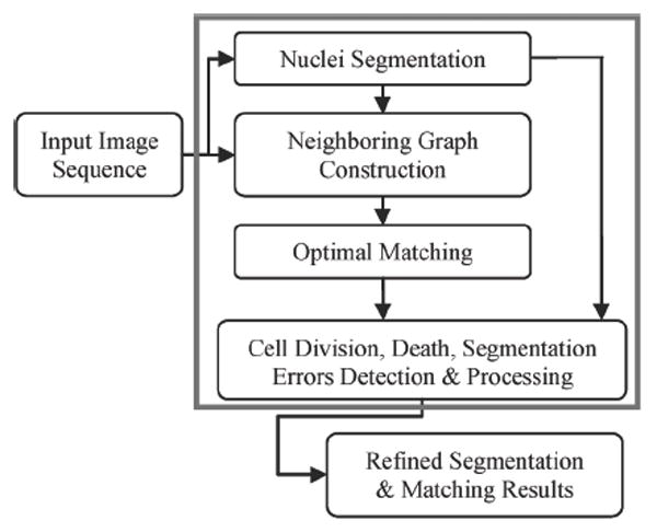
Overview flowchart of the proposed system.
II. Materials and Methodology
A. Materials
HeLa H2B-GFP cells were thawed six days before plating for each experiment and cultured in Dulbecco’s Modified Eagle Medium (DMEM) with 10% fetal bovine serum (FBS). All cells were plated in eight well #1 German borosilicate sterile bottomed plates (Nalge Nunc International) and incubated at 37°C in 5% CO2 for 18 h before imaging at 25 000 cells per well (50 000 cells per mL). Untreated cells were received medium while treated cells were received 300 nm nocodazole. Images were acquired on an automated epifluorescence TE2000-E Eclipse microscope (Nikon Instruments, Inc.) with a motorized XYZ-plane stage. Light was generated from a mercury arc lamp with two neutral density filters. Auto-focusingwas performed on the first pass and for every subsequent 10 passes to compensate for motor drift. Images were acquired using a 0.2 s exposure time, every 15 min for 50 h, yielding a total of 200 images for each position.
B. Methodology
1) Nuclei Segmentation
In this study, the nuclei detection and segmentation method proposed in [17] is employed. Essentially, this method consists of three components: binarization, nuclei center detection, and nuclei boundary delineating. We implemented the binarization process using an adaptive thresholding method [18]-[22]. Nuclei center detection is important because it determines the segmentation results by providing seed points for the seeded-watershed algorithm [17], [23]. To detect the centers of nuclei, we first utilize both intensity and shape information by combining the original intensity with the distance image as: I1 = I0 + αIDis, where I1 is the new image, I0 is the original image, and IDis is the distance image. The parameter α affects the nuclei center detection results by changing the relative weights of the intensity information (intensity image) and shape information (distance image). A high α value increases the influence of the distance image and a low α value decreases its influence. We empirically set α = 0.4 after testing a number of values on a training data set. The validation of how sensitive the parameter α affects the performance of the detection algorithm is provided in Section III-A. We detect the nuclei center using the gradient vector field(GVF)followed by Gaussian filtering [17], [24]. The pseudo-code for nuclei detection with GVF is as follows.
Algorithm (Nuclei Detection in GVF).
Mnuc; /*Nuclei pixel matrix. The background and nuclei pixels are set as 0 and 1 respectively*/
Mgvf; /*GVF matrix storing the gradient vectors of each pixel.*/
Mpar ← zeros(m,n); /*Particle convergence matrix, whose values are the number of virtual particles stopping at each pixel.*/
while (Exist Nonzero Element(Mnuc))
(x0, y0) ← Get One Nonzero Element(Mnuc); /*Get coordinates of one nonzero element (nuclei pixel) in Mnuc*/
(x1, y1) ← (0, 0);
-
while ((x1, y1)! = (x0, y0))
(x1, y1) ← Move Virtual Partial ((x0, y0), Mgvf(x0, y0)); /*Move the virtual particle from (x0, y0) along the gradient vector to the point (x1, y1). If pixel (x0, y0) is a local maximum, the gradient vector will point to itself, then the (x0, y0) and (x1, y1) are the same point.*/
end
Mpar(x1, y1) ← Mpar(x1, y1) + 1; /*Number of virtual particles at (x1, y1) increases one.*/
Mnuc(x0, y0) ← 0; /*Set the visited point as 0.*/
end
SeedsImage ← Thresholding (Mpar);
After detecting the nuclei centers, we delineate the nuclei boundaries using the seeded watershed algorithm. Fig. 2 provides representative detection and segmentation results.
Fig. 2.
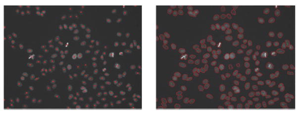
Representative detection and segmentation results of the proposed segmentation method.
2) Neighboring Graph Construction
The similar morphology of nuclei makes it difficult to accurately distinguish adjacent nuclei using only their morphological features. Therefore, we make use of the information of neighboring nuclei to better distinguish the adjacent nuclei. A way to describe the neighboring nuclei information is to connect the segmented nuclei into a neighboring graph. In the neighboring graph, the edges that connect nuclei with their neighbors can be used to characterize the spatial neighboring distribution, as seen in Fig. 3. However, this poses a critical question: how can we generate a neighboring graph that has strong ability to distinguish the adjacent nuclei using the neighboring relationships (spatial distribution of neighboring nuclei)? One possible solution is to connect all the neighbors of one nucleus, as shown in Fig. 3(a). However, it is difficult for a human observer to understand the neighboring relationships due to the complexity of this neighboring graph. In addition, more edges in the neighboring graph increase the computation time. Furthermore, the adjacent nuclei may have similar neighboring relationships and thus, it adds to the problem of distinguishing them from each other, as seen in Fig. 3(b) and (c). A different solution was proposed by Delaunay in 1934 Delaunay triangulation [25]. The representative neighboring graphs generated by using the Delaunay triangulation are provided in Fig. 3(d) and Fig. 4. As compared to the above neighboring graph, Delaunay neighboring graphs have less edges and are therefore easier to be understood, as seen in Fig. 3(d). Moreover, in such a graph the adjacent nuclei often have very different spatial distribution of neighboring nuclei that can be used to distinguish them easily, as seen in Figs. 3(e) and (f). These properties indicate that Delaunay triangulation technology is a good choice to generate the neighboring graph.
Fig. 3.
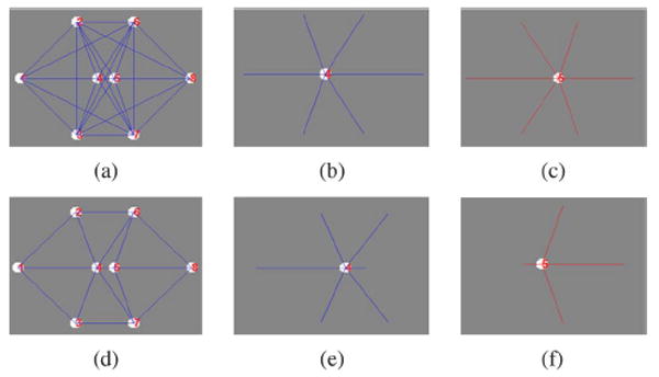
Example neighboring graphs. (a) Neighboring graph built by connecting any two nuclei; (b) and (c) are the edges connected to the fourth and fifth nuclei in neighboring graph (a). (d) Neighboring graph constructed by using the Delaunay triangulation method; (e) and (f) are the edges connected to the 4th and 5th nuclei in neighboring graph (d).
Fig. 4.
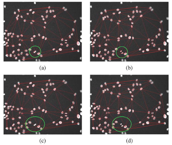
Illustration of the local variation of the neighboring graph caused by the cell division. (a) Neighboring graph in frame t; (b) neighboring graph in frame t +1 in which there is a cell division in the green box; (c) neighboring graph after removing the dividing cell in frame t; and (d) neighboring graph after removing the divided cells in frame t + 1.
3) Phase Controlled Optimal Matching
To match the segmented nuclei in two consecutive frames, we need to: 1) define a dissimilarity measure between two nuclei in two consecutive frames, and 2) choose an appropriate matching strategy.
a) Dissimilarity measure
The dissimilarity measure indicates how different two nuclei are and is critical for accurate nuclei matching. To define an appropriate dissimilarity measure, we first characterize a vertex (nucleus) in the kth neighboring graph (frame), vik, using an attribute vector: vik = (cik, sik, hik, eik), where cik = (xik, yik) denotes the centroid; sik is a binary matrix describing the shape of a nucleus, in which the nucleus and background are represented by 1 and 0, as seen in Fig. 5; hik is the intensity distribution of the nucleus, and we use the intensity histogram to represent the intensity distribution, as seen in Fig. 6; and is a 2 × M matrix that describes the spatial distribution (length and angle) of M edges connected to the nucleus in the neighboring graph, where θ is defined in radians, as shown in Fig. 7.
Fig. 5.
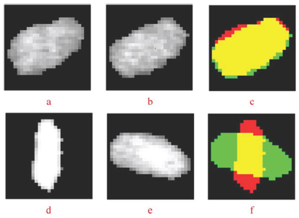
Illustration of measuring shape variability. (a), (b) Cropped and padded cellular images (matrixes) of the same nucleus in two consecutive frames. The corresponding binary matrixes have the same number of rows and columns as the cellular images. (c) Shows the calculation of shape variability; the yellow color indicates the intersection region; the red color indicates the complementary region of nucleus in (a); the green color indicates the complementary region of the nucleus in (b). (d), (e), (f) show the case of two different nuclei in two consecutive frames.
Fig. 6.
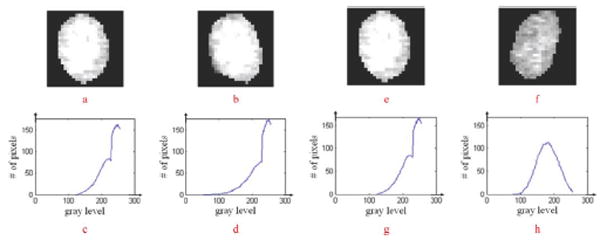
Illustration of measuring variation of intensity distribution. (a), (b) Same nuclei in two consecutive frames. (c), (d) Are their intensity histograms. (e), (f), (g), (h) Show the case of two different nuclei in two consecutive frames.
Fig. 7.
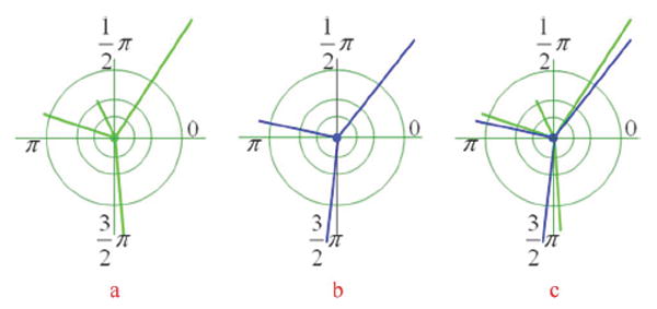
Illustration of measuring the variability of spatial distribution of neighboring nuclei. The green edges in (a) indicate the spatial distribution of neighboring nuclei of one nucleus in one frame, and the blue edges in (b) indicate the distribution of neighboring nuclei of the other nucleus in the next frame. (c) shows the difference of these two spatial distributions.
Based on the attribute vector, we define the dissimilarity measure between the ith nucleus in frame k and the jth nucleus in frame k + 1 as follows:
| (1) |
where αi, i = 1, 2, 3, 4 are the weighting parameters which satisfy αi ≥ 0, ; qi, i = 1, 2 are two phase control parameters, and we will describe them in detail after defining
| (2) |
the four normalized dissimilarity measures: , and .
The first term, , measures the Euclidean distance between the centroids of two nuclei, as show in (2) at bottom of the page where D denotes the maximum migration distance per frame, and we set D = 30 pixels empirically.
The second term, measures the nuclei shape variation which is defined as
| (3) |
Fig. 5 illustrates the calculation of nuclei the shape variation. The procedure of measuring the nuclei shape variation is as follows. After the initial nuclei segmentation we obtain a label matrix. In such a matrix, pixels within a nucleus region are labeled with a unique integer number which is used to distinguish it from other nuclei regions. We can obtain the binary matrix of a nucleus by cropping a small square region that contains the nucleus region tightly. Before comparing two binary matrices, we pad them symmetrically with zeros (background pixels) such that they have the same number of rows and columns. Then we can calculate their intersect region and union region based on (3).
The third term, , describes the variation of the intensity distribution
| (4) |
where max(I) and min(I) denote the maximum and minimum intensity values of the images. The numerator, of (4) measures the pixel number difference in tth gray level. In this study, we use min(I) = 0 and max(I) = 255. Fig. 6 shows two representative images of the variation of the intensity distribution using intensity histograms.
The last term, , measures the variation of the spatial distributions of neighboring nuclei. Without loss of generality, we assume that
| (5.1) |
| (5.2) |
In (5.1), is a collection of m edges selected from , and it enables the comparison between the spatial distributions with different edges. In (5.2), (m/n) measures the difference of edge number; compares the difference of the tth edge length; measures the variation of the tth edge angle; and the operation in (5.2) is to find the smallest difference between two spatial distributions of neighboring nuclei. Fig. 7 illustrates the variation of the spatial distributions of neighboring nuclei.
The determination of the optimal weighting parameters αi, i = 1, 2, 3, 4, is nontrivial as the validation of tracking results is time-consuming. Thus, we empirically tested a few values for αi, i = 1, 2, 3, 4, and selected the values with the highest tracking accuracy. In this study, we set them as: 0.31, 0.15, 0.23, and 0.31, with the ratio of them is roughly as 4 : 2 : 3 : 4. In Section III-B1, we provide a sensitivity analysis of αi, i = 1, 2, 3, 4. The validation results show that the tracking approach is robust to the parameters.
However, not all the four terms in the dissimilarity measure can be used, when the nuclei change from one phase to another regarding the following facts: 1) when the nuclei enter the prophase from the inter-phase their intensity increases dramatically, 2) when the nuclei enter the metaphase following the prophase, their shape changes dramatically, and 3) when cell divide the new generated cell nuclei will change the local structure of the neighboring graph around the dividing cells, as seen in the green circles of Fig. 4(a) and (b). To address problems 1) and 2), we add two phase control parameters: q1 and q2, to the shape and intensity terms. The two control parameters are defined as
| (6.1) |
| (6.2) |
where p(.) is a cell phase identification function. The details of the phase identification function can be found in [26]. The solution to problem (3) is described in the following section.
b) Matching strategy
The matching strategy associates (match) the nuclei in two consecutive frames based on the defined dissimilarity measure. In this study, we propose a division matching and 0-1 integer programming based optimal matching strategy.
To avoid that nuclei of dividing cells affect the neighboring graph, we first match the nuclei of dividing cells with the division matching strategy first and ignore them while we build the neighboring graph, illustrated with green circles of Fig. 4(c) and (d). Two observable facts of cell division are: 1) parent nucleus (Metaphase) divides along the direction perpendicular to its major axis [see Fig. 8(a) and (b)] and 2) two daughter nuclei (Anaphase) have similar appearances; see Fig. 8(b). Therefore, we need to find the parent nucleus of two daughter nuclei in a local region, as shown in the green rectangular boxes in Fig. 8(a) and (b). Specifically, this can be achieved by 1) finding all the nuclei which are in anaphase in frame (t +1) and placing them in a list Ld and 2) retrieving the first element in Ld, and checking if there is a sibling nucleus that satisfies , where dT is a dissimilarity threshold. If there is no sibling nucleus, the program checks the next element in Ld; otherwise, the program enters the next step; 3) checking if there exists a Metaphase nucleus in the desired local region in frame t. If the required nucleus exists, we match it with the two daughter nuclei. The steps 2 and 3 are repeated until all elements in Ld are checked.
Fig. 8.
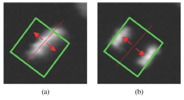
Illustration of the nuclei division.
After matching the dividing cells’ nuclei, the remaining nuclei are matched by the 0-1 integer programming based optimal matching strategy. The optimal matching problem is formulated as follows: let and denote two consecutive frames. For each nucleus, νik, in frame k, there are several matching candidates: . Therefore, a total of possible matches: exist. The optimal matching strategy, under the constraint that each nucleus has at most one match is to find a solution x0 = {0,1}N such that
| (7.1) |
| (7.2) |
In (7.2), x(t) denotes the tth element of vector x, and the term is the similarity of two nuclei. The matching constraints can be formulated as
| (7.3) |
where A is a (m + n) × N dimension “involving” matrix and b is a (m + n) elements vector of ones. In matrix A, the tth column corresponds to the tth possible match in M, t = 1, 2, …, N, indicating which nuclei correspond to that particular match
| (7.4) |
Obviously, this is a 0-1 integer programming problem. The linear programming based branch-and-bound (LPBB) algorithm is widely used to solve the 0-1 integer programming problem [27], [28]. The optimization process of LPBB is to build a searching tree by repeatedly discretizing (0 or 1) the variables (branching) and pruning the tree branches based on the optimal value of the node (bounding), computed by linear programming. In general, in a given search tree node the optimal value of the LP-relaxation problem at this node is greater than the existing best solution. The node and its branches will not be searched and a new node will be searched. If a new feasible 0-1 solution has a lower value, as compared with the existing best solution, the algorithm will update the existing best solution using the new feasible solution. If the value of the LP-relaxation problem at this node is less than that of the existing best solution, but it is not the 0-1 solution, two new searching tree nodes branching from this node are added by discretizing another variable (0 or 1), and the searching begins at a new node. The optimal solution is obtained by repeating the above process.
4) Cell Division, Death, Segmentation Errors Processing
Since the above optimal matching strategy is under the constraint that one nucleus matches at most once, there exist some nuclei with no match at all due to cell division, cell death (apoptosis), and segmentation errors (over- and under-segmentation). Although we have employed division matching to match all dividing cells’ nuclei, some nuclei are still missing due to the bias of the phase identification. We, however, can correct the segmentation errors and identify cell division and cell death by checking the remaining nuclei.
Cell division, over-segmentation, and bi-nucleus
A bi-nucleus is two inter-phase nuclei lying closely together such that they cannot be distinguished by the detection resolution of the microscopy, and thus appear as one nucleus in a few contiguous frames but eventually separate in the later frames, as seen in Fig. 9(a) and (b). When a bi-nucleus separates, a nucleus without match will be generated. Therefore, all the nuclei in frame t +1 which have no match are candidates of newly divided nuclei (in anaphase), newly separated bi-nuclei, or over-segmented nuclei, as seen in Fig. 9. Due to the distinct morphological appearances of the anaphase, bi-nuclei, and over-segmented nuclei, it is easy to separate them using a support vector machine (SVM) classifier based on the following six manually selected features: size, average intensity, standard deviation of intensity, compactness, long axis, and short axis. For the new divided nuclei and separated bi-nuclei candidates, we match them by finding the nuclei in frame t that are closest to them. For the over-segmented nuclei candidates, we merge them by finding the ones in frame t that overlap with them and have the smallest size.
Fig. 9.
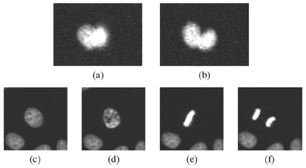
Bi-nuclei and four cell cycle phases. (a) Bi-nuclei; (b) separated bi-nuclei; (c) inter-phase; (d) prophase; (e) metaphase; and (f) anaphase.
Cell death (apoptosis) and under-segmentation
All the nuclei with no matching in frame are either the candidates for apoptotic cells or due to the under-segmentation of some nuclei in frame t +1. Therefore, we need to classify the candidates into the two groups: apoptosis and under-segmentation. Given a candidate , we find all its possible matching nuclei in frame t + 1 and then label the candidate as an apoptosis nucleus if there is no matching nucleus, which satisfies (under-segmentation)
| (8) |
where S(.) is the operator of calculating the area of a nucleus, and we empirically set α = 1.8. Otherwise, we label the nucleus , which satisfies (8) and has the largest size, as the under-segmented nucleus, and split it into two nuclei: and . We propose a splitting method to separate under-segmented nuclei, as shown in Fig. 10. After splitting, we can easily match the two split nuclei and with and .
Fig. 10.

Illustration of the proposed nuclei splitting method.
III. Validation Results
A. Validation of Segmentation
Unlike cell cytoplasmic images with complex shapes and significant intensity variations, cell nuclei have regular shape and uniform intensity. If the cell nuclei centroids are detected correctly, the cell boundaries will be well delineated, as shown in Fig. 2. Thus, it is reasonable to validate the segmentation by just counting the over-segmentation errors (two or more detected nuclei centroids are presented inside one nucleus region) and under-segmentation errors (two or more nuclei regions share only one detected centroid).
1) Sensitivity Analysis of Parameter α in Nuclei Detection
To validate how the sensitivity of the parameter α affects the detection performance, we uniformly selected 21 nuclei images from each of four nuclei image sequences (frames 1, 10, 20, …, 200 are selected). These 84 (21 × 4) nuclei images contain about 8300 nuclei. We used two error measures to evaluate the performance of the detection approach: over-detection (the same as the over-segmentation) and under-detection errors (the same as the under-segmentation). We varied the value of α from 0 to 1. The detailed results of the detection algorithm are provided in Table I. As we can see, the over-detection error is more sensitive to the variation of the value of α as compared to the under-detection error. If we increase α to 1, both over-detection and under-detection increase. From 0.2 to 0.6, the detection algorithm keeps the similar error rate. From 0 to 0.8, the error rate is confined within 1%. In conclusion, the detection approach is robust to the parameter α.
TABLE I.
Sensitivity Validation of Parameter α in Nuclei Detection
| α | 0 | 0.2 | 0.3 | 0.4 | 0.5 | 0.6 | 0.8 | 1 |
|---|---|---|---|---|---|---|---|---|
| Over- detection | 53 | 41 | 42 | 42 | 45 | 53 | 64 | 83 |
| Under- detection | 18 | 18 | 15 | 14 | 14 | 10 | 13 | 22 |
| Errors Rate (%) | 0.86 | 0.71 | 0.69 | 0.67 | 0.71 | 0.76 | 0.93 | 1.3 |
2) Comparison of Nuclei Segmentation
Two cell sequences were selected to evaluate the proposed segmentation method with the manual detection results were used as the ground truth. The detailed validation results are provided in Table II. The first sequence contained a total of 18 683 nuclei. Using the proposed method, 35 nuclei were over-segmented and 84 nuclei were under-segmented. The second sequence contained 19, 469 nuclei. Using our method, 40 nuclei were over-segmented and 30 nuclei were under-segmented. On average, the segmentation accuracy is very high and reaches 99.50%.
TABLE II.
Validation of Segmentation Results
| Seq. | # of nuclei | Correctly segmented | Over-segmented | Under-segmented |
|---|---|---|---|---|
| 1 | 18683 | 18564 (99.36%) | 35 (0.19%) | 84 (0.45%) |
| 2 | 19469 | 19394 (99.61%) | 40 (0.21%) | 35 (0.18%) |
| Total | 38152 | 37963 (99.50%) | 75 (0.20%) | 119 (0.30%) |
To further validate the segmentation algorithm, we compared the proposed segmentation method with the watershed algorithm [23] and the watershed-based hybrid merging algorithm [29]. Table III shows the detailed comparison results. The hybrid merging algorithm improved the segmentation accuracy from 87% to 94.69% compared with the watershed algorithm, and the segmentation accuracy of our proposed method is even 5% higher than that of the hybrid algorithm.
TABLE III.
Comparison of Segmentation Results Using Nuclei Image Sequence 1
| Methods | Correctly segmented | Over-segmented | Under-segmented |
|---|---|---|---|
| Watershed | 16254 (87%) | 2242 (12%) | 187 (1%) |
| Watershed/Hybrid | 17690 (94.69%) | 747 (4%) | 246 (1.32%) |
| Detection/Watershed | 18564 (99.36%) | 35 (0.19%) | 84 (0.45%) |
B. Validation of Tracking
In this study, a trace is defined as a path beginning from an ancestor cell nucleus in the first frame to its descendant cell nucleus in the last frame. Nuclei in the trace reflect the position and morphological appearance changing over time. A match means an association between two nuclei in two consecutive frames. Therefore, a trace consists of N − 1 matches, where N is the length of the cellular image sequence. To validate the proposed tracking method, we define two error rates, namely, error trace rate (ETR) and error match rate (EMR), as follows: ETR = # of error traces/# of total traces, and ETR = # of error matches/# of total traces. We label a trace as an error trace if there is at least one match error. The low ETR cannot guarantee high match accuracy because one error trace maybe contains many error matches. Similarly, low EMR does not mean high tracking accuracy because each error trace may just contain one error match. On the other hand, an error match in the parent nuclei will result in consecutive errors of all traces branching from it. Only when both, the error trace rate and error match rate are low we can say that the tracking system is reliable.
1) Sensitivity Analysis of Parameters {α1, α2, α3, α4} in Nuclei Tracking
To test how sensitive the variations of the parameters affect the performance of the tracking algorithm, we designed the following experiments: four nuclei image sequences were selected to validate the proposed tracking algorithm. For each sequence, the values of {α1, α2, α3, α4} were generated as follows: 1) randomly generate four numbers in ±[0.01, 0.05]; 2) get new values of {α1, α2, α3, α4} by adding these four random numbers to [0.31, 0.15, 0.23, 0.31]; and 3) normalize the new values such that and perform the tracking procedure with the new generated parameters’ setting {α1, α2, α3, α4}. The detailed tracking validation results are provided in Table IV. Compared with the tracking results under the original parameter setting, see Table V, we conclude that the random variations of the parameters {α1, α2, α3, α4} do not influence much on the performance of the proposed tracking approach. We further investigated these tracking errors occurred under the newly generated parameters and that under the original setting. As seen in Table VI, the error traces and error matches under different parameter variations are almost the same as that under the original parameter setting. In conclusion, the tracking approach is robust to the parameters {α1, α2, α3, α4}.
TABLE IV.
Tracking Validation Results Under Different Variations of {α1, α2, α3, α4}
| Seq. | Values of {α1, α2, α3, α4} | # of cell traces | ETR | EMR |
|---|---|---|---|---|
| 1 | [0.33, 0.16, 0.19, 0.32] | 97 | 7 (7.22%) | 6 (6.18%) |
| 2 | [0.34, 0.13, 0.20, 0.33] | 109 | 17 (15.59%) | 15 (13.76%) |
| 3 | [0.28, 0.13, 0.25, 0.34] | 107 | 10 (9.35%) | 11 (10.28%) |
| 4 | [0.32, 0.19, 0.21, 0.28] | 131 | 12 (9.16%) | 11 (8.40%) |
| Total | 444 | 46 (10.36%) | 43 (9.68%) |
TABLE V.
Comparison of Nuclei Tracking Results
| Seq. | Proposed tracking method | Location and size based tracker | ||||
|---|---|---|---|---|---|---|
| # of cell traces | ETR | EMR | # of cell traces | ETR | EMR | |
| 1 | 97 | 7 (7.22%) | 6 (6.18%) | 109 | 36 (33.03%) | 47 (43.12%) |
| 2 | 109 | 16 (14.68%) | 15 (13.76%) | 116 | 51 (43.97%) | 56 (48.28%) |
| 3 | 107 | 9 (8.41%) | 9 (8.41%) | 111 | 48 (43.24%) | 51 (45.95%) |
| 4 | 131 | 12 (9.16%) | 11 (8.40%) | 128 | 61 (47.66%) | 56 (43.75%) |
| Total | 444 | 44 (9.91%) | 41 (9.23%) | 464 | 196 (42.24%) | 210 (45.26%) |
TABLE VI.
Comparison of the Differences Between the Error Traces and Error Matches Occurred Under the Variations of Parameters {α1, α2, α3, α4} and that Occurred Under the Original Setting
| Seq. | Common Error Traces | Different Error Traces | Common Error Matches | Different Error Matches |
|---|---|---|---|---|
| 1 | 7 | 0 | 6 | 0 |
| 2 | 16 | 1 | 15 | 0 |
| 3 | 9 | 1 | 9 | 2 |
| 4 | 12 | 0 | 11 | 0 |
| Total | 44 | 2 | 41 | 2 |
2) Comparison of Nuclei Tracking
We compared the proposed method with a location and size based tracker used in [29]. In summary, the location and size based tracker first defines a dissimilarity measure based on the overlapping area and the distance of the centroids of two nuclei in two consecutive frames. Then it matches the nuclei one by one based on the defined dissimilarity measure. We provide the detailed comparison results in Table V. On average about 90% of nuclei traces obtained from the proposed method are correct, and both the ETR and EMR are restricted to 10%. Whereas both the ETR and EMR of the location and size based tracker are 30% higher than the proposed tracking method. Through further investigation, we found that fast moving and cell division cause the most nuclei matching errors for the location and size based tracker while the proposed system deals with these challenges well. In conclusion, the proposed tracking method is accurate and reliable.
C. Extracted Cell Trajectories
In Fig. 11, we illustrate the representative 2-D HeLa cell migration maps, in which different cell migration traces are represented by different colors. As we can see, some cells move in a small region (shown inside the red square box), and some cells migrate farther out (shown in the blue square box). In the anti-cancer drug screening study, the analysis of cell cycle time distribution is important. The drugs or commands that can prolong the time of the cell cycle could be new candidates for anti-cancer treatment. In Fig. 12, the division progression of a nucleus is shown. There are three cell divisions at T = 3.75, 27.5, and 28.5 h, respectively, as shown in Fig. 13(b). We also can see that the cell cycle progression of daughter nuclei may have different cell division rates, as seen in Fig. 13(a). In addition, three representative 3-D cell nuclei trajectories extracted automatically are shown in Fig. 14, in which we can clearly see both the cell migration and cell division information.
Fig. 11.
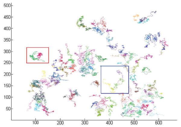
Two-dimensional cell migration traces.
Fig. 12.
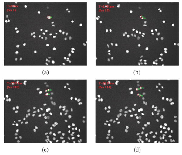
Illustration of cell division. (a) The #28 nucleus in the first frame; (b) the #28 nucleus divided in frame 15, and the two daughter nuclei are #30 and #33, respectively; and (c) the daughter nuclei #30 and #33 divided in frames 110 and 114, respectively.
Fig. 13.
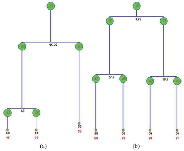
Tree structure of cell cycle progression. The red numbers in green notes are the number of nuclei; the black numbers denote the division time (in hours); the red numbers at bottom is the number of traces. (a) Tree structure of a cell cycle progression in which the cell cycle progression of the daughter nuclei are different and (b) the tree structure of cell cycle progression of the cell in Fig. 10.
Fig. 14.
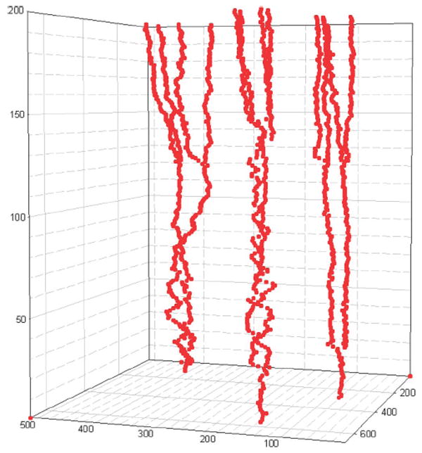
Three representative 3-D cell trajectories that are extracted automatically.
D. DCellIQ Software Package
We incorporated the proposed tracking method into a software package: DCellIQ (Dynamic CELLular Image Quantitator), which is designed specifically for the analysis of cell cycle progression and dynamics. In DCellIQ system, cell nuclei segmentation, tracking, and cell cycle phase identification are preformed automatically. The software can be downloaded freely at our website.1
IV. Conclusion
Cell cycle behavior analysis of cancer cells is important for understanding the mechanisms of anti-cancer drugs and for the screening of new drugs. However, the significant challenge in quantifying the time-lapse cellular images has been becoming the bottleneck of cell cycle progression analysis. In this paper, we present a fully automated segmentation and tracking method for quantifying time-lapse cellular images. A cell detector that combines the shape and intensity information is implemented to separate the clustered nuclei. We view the nuclei as vertices in the neighboring graph that is generated using the Delaunay triangulation. We improve the tracking accuracy by defining a new dissimilarity measure that takes into account the morphological appearance, migration distance, and neighboring relationship using phase information. Then, we develop the division matching and optimal matching strategy to match the nuclei of two consecutive frames. Finally, the segmentation errors, cell division, and death are further processed. The experimental results show that the proposed segmentation and tracking method is accurate and reliable. Therefore, we incorporated the proposed method into a public domain software package, DCellIQ.
Acknowledgments
The authors would like to acknowledge Dr. R. King from Harvard University who provided the initial datasets for this study and thank Dr. S. K. Choy and Mr. D. Beck for their suggestions during manuscript preparation.
This work was supported by the National Institutes of Health under Grant NIH R01 LM008696. The work of S. T. C. Wong was supported by the Center for Bioinformatics Program Grant of Harvard Center of Neurodegeneration and Repair (now Harvard Neurodiscovery Center), Harvard Medical School.
Footnotes
Contributor Information
Fuhai Li, Department of Information Science, School of Mathematical Sciences, and LMAM, Peking University, Beijing 100871, China. He is now with the Bioinformatics and Biomedical Engineering Programmatic Core, and Research Division, Department of Radiology, The Methodist Hospital Research Institute, Weill Medical College, Cornell University, Houston, TX 77030 USA (robert.fh.li@gmail.com).
Xiaobo Zhou, Bioinformatics and Biomedical Engineering Programmatic Core, and Research Division, Department of Radiology, The Methodist Hospital Research Institute, Weill Medical College, Cornell University, Houston, TX 77030 USA (xzhou@tmhs.org).
Jinwen Ma, Department of Information Science, School of Mathematical Sciences, and LMAM, Peking University, Beijing 100871, China (jwma@math.pku.edu.cn).
Stephen T. C. Wong, Bioinformatics and Biomedical Engineering Programmatic Core, and Research Division, Department of Radiology, The Methodist Hospital Research Institute, Weill Medical College, Cornell University, Houston, TX 77030 USA (xzhou@tmhs.org; stwong@tmhs.org)
References
- 1.Haggarty S, Mayer T, Miyamoto D, et al. Dissecting cellular processes using small molecules: Identification of colchicine-like, taxol-like and other small molecules that perturb mitosis. Chem Biol. 2000;7:275–286. doi: 10.1016/s1074-5521(00)00101-0. [DOI] [PubMed] [Google Scholar]
- 2.Williams NS, Burgett AWG, Atkins AS, et al. Therapeutic anticancer efficacy of a synthetic diazonamide analog in the absence of overt toxicity. Proc Nat Acad Sci. 2006;104:2074–2079. doi: 10.1073/pnas.0611340104. [DOI] [PMC free article] [PubMed] [Google Scholar]
- 3.Zhou X, Wong STC. Informatics challenges of high-throughput microscopy. IEEE Signal Process Mag. 2006;23(3):63–72. [Google Scholar]
- 4.Loo LH, Wu LF, Altschuler SJ. Image-based multivariate profiling of drug responses from single cells. Nature Meth. 2007 May;4(5):445–453. doi: 10.1038/nmeth1032. [DOI] [PubMed] [Google Scholar]
- 5.Zhou X, Wong STC. High content cellular imaging for drug development. IEEE Signal Process Mag. 2006 Mar;23(2):170–174. [Google Scholar]
- 6.Chen X, Zhou X, Wong STC. Automated segmentation, classification, and tracking of cancer cell nuclei in time-lapse microscopy. IEEE Trans Biomed Eng. 2006 Apr;53(4):762–766. doi: 10.1109/TBME.2006.870201. [DOI] [PubMed] [Google Scholar]
- 7.Li K, Miller ED, Weiss LE, et al. Online tracking of migrating and proliferating cells imaged with phase-contrast microscopy. Proc. Conf. Comput. Vis. Pattern Recognit Workshop; New York. 2006. p. 65. [Google Scholar]
- 8.Al-Kofahi O, Radke RJ, Goderie SK, et al. Automated cell lineage construction. Cell Cycle. 2006;5(3):327–335. doi: 10.4161/cc.5.3.2426. [DOI] [PubMed] [Google Scholar]
- 9.Cheng Y. Mean shift, mode seeking, and clustering. IEEE Trans Pattern Anal Mach Intell. 1995 Aug;17(8):790–799. [Google Scholar]
- 10.Debeir O, Ham PV, Kiss R, et al. Tracking of migrating cells under phase-contrast video microscopy with combined mean-shift processes. IEEE Trans Med Imag. 2005 Jun;24(6):697–711. doi: 10.1109/TMI.2005.846851. [DOI] [PubMed] [Google Scholar]
- 11.Nilanjan R, Acton ST, Ley K. Tracking leukocytes in vivo with shape and size constrained active contours. IEEE Trans Med Imag. 2002 Oct;21(10):1222–1235. doi: 10.1109/TMI.2002.806291. [DOI] [PubMed] [Google Scholar]
- 12.Kass M, Witkin A, Terzopoulos D. Snake: Active contour models. Int J Comput Vis. 1987;1(4):321–331. [Google Scholar]
- 13.Xu C, Prince JL. Snakes, shapes, and gradient vector flow. IEEE Trans Image Process. 1998 Mar;7(3):359–369. doi: 10.1109/83.661186. [DOI] [PubMed] [Google Scholar]
- 14.Malladi R, Sethian AJ, Vemuri B. Shape modeling with front propagation: A level set approach. IEEE Trans Pattern Anal Mach Intell. 1995 Feb;17(2):158–175. [Google Scholar]
- 15.Mukherjee DP, Ray N, Acton ST. Level set analysis for leukocyte detection and tracking. IEEE Trans Image Process. 2004 Apr;13(4):562–572. doi: 10.1109/tip.2003.819858. [DOI] [PubMed] [Google Scholar]
- 16.Zimmer C, Labruyère E, Meas-Yedid V, et al. Segmentation and tracking of migrating cells in videomicroscopy with parametric active contours: A tool for cell-based drug testing. IEEE Trans Med Imag. 2002 Oct;21(10):1212–1221. doi: 10.1109/TMI.2002.806292. [DOI] [PubMed] [Google Scholar]
- 17.Li F, Zhou X, Zhu J, et al. High content image analysis for H4 human neuroglioma cells exposed to CuO nanoparticles. BMC Biotechnol. 2007;7:66. doi: 10.1186/1472-6750-7-66. [DOI] [PMC free article] [PubMed] [Google Scholar]
- 18.Otsu N. A threshold selection method from gray-level histograms. IEEE Trans Syst, Man, Cybern. 1979 Jan;9(1):62–66. [Google Scholar]
- 19.Adiga U, Malladi R, Fernandez-Gonzalez R, et al. High-throughput analysis of multispectral images of breast cancer tissue. IEEE Trans Image Process. 2006 Aug;15(8):2259–2268. doi: 10.1109/tip.2006.875205. [DOI] [PubMed] [Google Scholar]
- 20.Wahlby C, Lindblad J, Vondrus M, et al. Algorithms for cytoplasm segmentation of fluorescence labelled cells. Analyt Cell Pathol. 2002;24(2–3):101–111. doi: 10.1155/2002/821782. [DOI] [PMC free article] [PubMed] [Google Scholar]
- 21.Lindblad J, Wahlby C, Bengtsson E, et al. Image analysis for automatic segmentation of cytoplasms and classification of Rac1 activation. Cytometry A. 2004 Jan;57(1):22–33. doi: 10.1002/cyto.a.10107. [DOI] [PubMed] [Google Scholar]
- 22.Sezgin M, Sankur B. Survey over image thresholding techniques and quantitative performance evaluation. J Electron Imag. 2004;13(1):146–165. [Google Scholar]
- 23.Vincent L, Soille P. Watersheds in digital spaces: An efficient algorithm based on immersion simulations. IEEE Trans Pattern Anal Mach Intell. 1991 Jun;13(6):583–598. [Google Scholar]
- 24.Lindeberg T. Feature detection with automatic scale selection. Int J Comput Vis. 1998;30(2):79–116. [Google Scholar]
- 25.O’Rourke J. Computational Geometry in C. Second Edition. New York: Cambridge Univ Press; 1998. [Google Scholar]
- 26.Wang M, Zhou X, King RW, et al. Context based mixture model for cell phase identification in automated fluorescence microscopy. BMC Bioinform. 2007;8:32. doi: 10.1186/1471-2105-8-32. [DOI] [PMC free article] [PubMed] [Google Scholar]
- 27.Nemhauser GL, Wolsey LA. Integer and Combinatorial Optimization. New York: Wiley; 1988. [Google Scholar]
- 28.Wolsey LA. Integer Programming. New York: Wiley; 1998. [Google Scholar]
- 29.Yan J, Zhou X, Yang Q, et al. An effective system for optical microscopy cell image segmentation, tracking and cell phase identification. Proc. IEEE Int. Conf. Image Process; Atlanta, GA. 2006. pp. 1917–1920. [Google Scholar]


