Drinking Typography Established by Scheduled Induction Predicts Chronic Heavy Drinking in a Monkey Model of Ethanol Self-Administration

Abstract

Background

We have developed an animal model of alcohol self-administration that initially employs schedule-induced polydipsia (SIP) to establish reliable ethanol consumption under open access (22 h/d) conditions with food and water concurrently available. SIP is an adjunctive behavior that is generated by constraining access to an important commodity (e.g., flavored food). The induction schedule and ethanol polydipsia generated under these conditions affords the opportunity to investigate the development of drinking typologies that lead to chronic, excessive alcohol consumption.

Methods

Adult male cynomolgus monkeys (Macaca fascicularis) were induced to drink water and 4% (w/v in water) ethanol by a Fixed-Time 300 seconds (FT-300 seconds) schedule of banana-flavored pellet delivery. The FT-300 seconds schedule was in effect for 120 consecutive sessions, with daily induction doses increasing from 0.0 to 0.5 g/kg to 1.0 g/kg to 1.5 g/kg every 30 days. Following induction, the monkeys were allowed concurrent access to 4% (w/v) ethanol and water for 22 h/day for 12 months.

Results

Drinking typographies during the induction of drinking 1.5 g/kg ethanol emerged that were highly predictive of the daily ethanol intake over the next 12 months. Specifically, the frequency in which monkeys ingested 1.5 g/kg ethanol without a 5-minute lapse in drinking (defined as a bout of drinking) during induction strongly predicted (correlation 0.91) subsequent ethanol intake over the next 12 months of open access to ethanol. Blood ethanol during induction were highly correlated with intake and with drinking typography and ranged from 100 to 160 mg% when the monkeys drank their 1.5 g/kg dose in a single bout. Forty percent of the population became heavy drinkers (mean daily intakes >3.0 g/kg for 12 months) characterized by frequent “spree” drinking (intakes >4.0 g/kg/d).

Conclusion

This model of ethanol self-administration identifies early alcohol drinking typographies (gulping the equivalent of 6 drinks) that evolve into chronic heavy alcohol consumption in primates (drinking the equivalent of 16 to 20 drinks per day). The model may aid in identifying biological risks for establishing harmful alcohol drinking.

Alcohol abuse and alcoholism represent significant public health concerns recognized throughout the world. In the United States, the Centers for Disease Control and Prevention has ranked alcohol abuse the number 3 preventable cause of death in the country (Mokdad et al., 2004). The current estimate of the number of Americans who meet the diagnostic criteria of alcohol abuse or dependence is 18 million or 8.5% of the population 18 years and older (Grant et al., 2004). Heavy alcohol consumption (greater than 6 drinks per day, >1.5 g/kg, and 20% of daily calories in the form of alcohol) is comorbid with brain, heart, lung, liver, pancreatic and kidney disease states, and is a cofactor in cancer, reproductive and immune system dysfunction (Gunzerath et al., 2004). Although nearly all individuals in the United States are exposed to alcohol, consumption of alcohol is unevenly distributed, with 64% of the adult U.S. population actively drinking alcohol and 20%of this population consuming approximately 80% of all the alcohol sold (Dawson, 2000). Thus, individuals are not at equal risk for drinking alcohol excessively. Research directed at predicting which individuals are at high risk for alcoholism is a matter of urgent public health concern for the development of prevention and harm-reduction programs.

At present, the relative contributions of risk factors that prompt some individuals to drink alcohol excessively are not known, although sex, age of onset of drinking, social networks, genetics, availability, and stressful events have all been implicated. Animal models of human disease are commonly used to identify and assess etiological factors, including diseases that involve a large behavioral component such as alcohol abuse and alcoholism. Among the different animals used in alcohol research, nonhuman primates are important subjects because of their genetic homology with humans, their propensity to self-administer large quantities of alcohol (ethanol) orally, and their absorption and metabolism of ethanol that are similar to humans (Grant and Bennett, 2003).

Despite the rigorous control that nonhuman primates offer in studies assessing risk for alcohol abuse and alcoholism, the characterization of voluntary and excessive ethanol drinking in monkeys has been very limited. Particularly sparse are data that capture accurate consumption patterns of chronic intake in the range of 12 to 24 drinks per day (>3.0 to 6.0 g/kg) for periods of time encompassing months or years. In humans, periods of heavy alcoholic drinking are often described as “benders” or “sprees” and the resultant intoxication is associated with many adverse outcomes such as traffic fatalities, violent behavior, and biomedical complications. Binges are currently defined as drinking 5 or more alcoholic drinks on an occasion and are the target for harm-reduction policies (Dawson, 2000). However, studies on the patterns of drinking in alcoholics given unlimited access to alcohol have reported sprees (or benders) of much more excessive intake consisting of approximately 1 quart of distilled alcohol, such as bourbon, a day (roughly 22 to 24 drinks) for several consecutive days (Majchrowicz, 1977; Majchrowicz and Mendelson, 1970; Mello and Mendelson, 1970; Nathan et al., 1971). A perhaps crucial factor in alcoholic binging is the desire to increase alcohol consumption far above an already substantial baseline of intake. For many reasons, direct laboratory studies of human alcoholic drinking have been curtailed since the 1970s and today most studies rely on self-report of drinks per drinking days (Stahre et al., 2006). Without direct studies of chronic, alcoholic drinking under unlimited access, many fundamental questions concerning individual risk for, and the biological basis of, excessive ethanol consumption remain unanswered.

We have utilized a model of oral ethanol self-administration in monkeys that results in a high proportion (approximately 35%) of heavy drinking individuals that averaged daily ethanol intakes of 3.0 g/kg per day (>12-drink equivalent) for 12 months with frequent episodes of spree drinking that fit the characteristics of human alcoholic spree drinking. The monkeys attain blood ethanol concentrations (BEC) between 100 and 400 mg/dl when measured 7 to 8 hours after the onset of drinking (Vivian et al., 2001) and metabolize ethanol at rates similar to human beings (Green et al., 1999). These daily intakes and BECs are similar to those reported for alcoholic men who were given 20 to 60 consecutive days of free access to ethanol 24 h/d (Majchrowicz and Mendelson, 1970; Mello and Mendelson, 1970, 1971; Nathan et al., 1971). In this procedure, we utilize a schedule-induction procedure to initiate ethanol self-administration. Induction procedures are necessary in animal models of ethanol self-administration because in a vast majority of the studies simply allowing access to ethanol is not sufficient to result in repeated consumption of intoxicating quantities. The low levels of ethanol intake of uninitiated animals have been attributed to the taste of alcohol, the delay between the consumption of alcohol and its pharmacological effects, the volume of alcohol needed for a pharmacological effect, and the particular pharmacological effects of alcohol (including positively reinforcing as well as aversive effects). To circumvent these difficulties, it is now standard to use an induction procedure to establish ethanol drinking in animals that have not been specifically bred to drink large amounts of an alcohol solution. Induction procedures include food deprivation, adulterating the taste of ethanol, associating the consumption of ethanol with the presentation or removal of other reinforcers, acclimating the animal to gradually increasing concentrations of ethanol, and restricting access to the alcohol solution (see Meisch, 1984; Rhodes et al., 2005; Samson, 1987).

We previously published data on the following cohort of monkeys showing baseline deoxycorticosterone and pregnenolone response to a dexamethasone challenge correlated with average ethanol intakes over the next 12 months of ethanol self-administration (Pearson R = −0.78, p < 0.006; Porcu et al., 2005, 2006). These results were from assays taken prior to induction. The objective of the following experiment was to characterize a large number of behavioral and organismal variables related to drinking during the initial exposure to alcohol and determine which, if any, variables could predict which monkeys would become chronic and heavy drinkers. For the initial exposure to drinking ethanol, the monkeys were placed under a schedule-induction procedure. Schedule-induced drinking occurs when a fluid is available and access to food is restricted, with small quantities of food delivered intermittently at fixed intervals of time (Falk, 1993; Sanger, 1986). Schedule-induced drinking was first reported in 1961 when it was observed that food-deprived rats allowed access to small quantities of food under an intermittent schedule drank water in amounts equivalent to nearly half of their body weight in a 3-hour period (Falk, 1961). Under schedule-induction conditions, drinking is neither required nor explicitly reinforced. Nevertheless, animals persistently drank large volumes of fluid when the interval between pellet delivery lies somewhere between freely available and very long, usually 3 to 20 minutes (Allen and Kenshalo, 1978; Byrd, 1980; Grant and Johanson, 1988; Porter and Kenshalo, 1974; Schuster and Woods, 1966). Peak adjunctive drinking of water ranged from 463 to 840 ml/h in rhesus monkeys (Allen and Kenshalo, 1976; Schuster and Woods, 1966) to 281 to 365 ml/h in cynomolgus monkeys (Allen and Kenshalo, 1978). Indeed, nonhuman primates appear to be easily susceptible to schedule-induced polydipsia (SIP), and can be induced by the intermittent delivery of food pellets without food deprivation (Grant and Johanson, 1988).

Schedule-induced procedures have been used to induce large volumes of ethanol consumption in rats, monkeys, and humans (see Doyle and Samson, 1985; Meisch, 1984; Samson, 1987). Indeed, there is a wealth of data that suggest specific parameters for obtaining physical dependence and high blood alcohol levels using SIP in rodents (for reviews see, Falk, 1971, 1993). It appears that the optimal concentration of ethanol that rodents can be induced to drink is 5% v/v ethanol (Falk et al., 1972) and the optimal schedule is a 2-minute fixed-time (FT) interval of pellet presentation (Falk, 1966; Falk et al., 1972; Samson and Falk, 1975). In cynomolgus monkeys, we determined that 4% (w/v) ethanol and 5 minutes is an optimal FT interval schedule of food pellet delivery to induce consumption of 1.0 g/kg ethanol (Shelton et al., 2001). That is, all monkeys exposed to the 5 minute interval schedule using 4% (w/v) ethanol were induced to drink the 1.0 g/kg dose. Furthermore, we used these schedule parameters to establish ethanol self-administration for over a year in monkeys kept at their free-feeding weight (Vivian et al., 2001).

In the following procedure, after the induction of ethanol self-administration, monkeys were immediately placed under “open access” conditions and given a choice of ethanol (4% w/v) or water to drink for 22 h/d, 7 d/wk for 12 months. The daily average ethanol intake (gram ethanol per kg body weight per day) over the 12 months of open access served as the major correlate and outcome measure in searching for predictions of future heavy drinking (operationally defined as an average of >3.0 g/kg/d, Vivian et al., 2001).

MATERIALS AND METHODS

Animals

Monkeys (Macaca fascicularis, 50 to 62 months of age, weight 3.84 to 5.74 kg, n = 10) were purchased from a commercial vendor (World Wide Primates, Miami, FL) and placed into a CDC quarantine facility for 2 months upon arrival at Wake Forest University School of Medicine. Upon release from quarantine, the monkeys lived in the laboratory with visual, auditory, and olfactory contact with other conspecifics. The monkeys were housed individually in quadrant cages (1.6 × 0.8 × 0.8 m) in a room with constant temperature (68 to 72°F), humidity (65%) and a 12 hour light cycle (lights on at 7:00 AM). For the duration of the entire experiment the monkeys were weighed weekly.

During the first month, the monkeys were acclimated to the laboratory personnel, then trained to provide their leg through an opening in the cage front for awake blood collection via saphenous or femoral venipuncture for the assays of cortisol, dexycorticosterone, ACTH, and ethanol (Porcu et al., 2005). Each step in the behavioral training was considered complete when the animals performed the behavior readily and with minimal observable distress. Briefly, twice a day each monkey was trained with positive reinforcement (giving fresh fruit) to move to the front of the cage and present its leg through an opening in the cage (10 × 10 cm). As the animal became comfortable with this behavior, the animal’s upper leg at the femoral triangle was lightly pricked with a dental pick to simulate a needle stick before advancing to the actual blood draw. Once the animal was comfortable with this, a 3 cc blood sample was drawn through a 22-guaged needle into an EDTA-coated vacutainer tube. All primate handling procedures were performed in accordance with the NIH and were approved by Wake Forest University ACUC in accordance with the Commission on Life Sciences, National Research Council (1996) Guide for the Care and Use of Laboratory Animals (National Academy Press, Washington).

Apparatus

Attached to one wall of each monkey’s home cage was an operant panel that allowed access to all fluid and food via a response on a push panel. These panels were controlled by a computerized system (Macintosh G4, Apple Computer, Inc. Cupertino, CA, with National Instruments hardware and programming environment, National Instruments Corporation, Austin, TX). They contained 2 drinking spouts, a set of 3 lights (red, white, and green) positioned above each spout, one push panel (with a red stimulus light LED) positioned below one of the spouts, and a centrally positioned opening containing a dowel with an associated white stimulus light. Each spout extended approximately 4 cm into the cage and was connected via tubing to a 1 l fluid reservoir located on top of a digital scale (Ohaus Navigator Balances N1B110, Ohaus Corporation, Pine Brook, NJ). Drinking data were obtained by placing 1-l fluid containers on scales, and then retrieving weight values through serial communication with the scales. Both 1 ml water and 1 ml 4% (w/v) ethanol weighed 1 g/ml; thus, the resolution of mass displacement from the scale was set at 0.1 g (or 0.1 ml fluid). The resolution of time for calculating rates of drinking was approximately 500 milliseconds across all 10 panels operated simultaneously.

Induction of Ethanol Self-Administration

Monkeys were trained to operate the drinking panel in daily 60-minutes sessions and then induced to drink water and later ethanol (4% w/v in water). An active panel, fluid, and food availability was signaled through illumination of the white, green, and red stimulus lights, respectively. Initially, fluid was available through a single drinking spout, and 1 press on the push panel resulted in delivery of a 1-g banana-flavored pellet (Research Diets Incorporated, New Brunswick, NJ). Monkeys were trained to press the panel for food delivery for their meals; responding was not required in the FT delivery of pellets. Training was complete (approximately 2 to 3 weeks) once the monkey reliably drank from the spout, and received all available food pellets by responding on the push panel.

The session variables were controlled by a computer program (BioticMicro, Clemmons, NC) that created a “record,” each time a pellet was delivered, drinking occurred (fluid displacement measured), or a specific condition took place, such as achieving the required induction volume. Drinking records were defined as a “drink” (continuous fluid displacement with less than 5 seconds between records) and a “bout” (less than 5 minutes between records) and numbered consecutively to evaluate the temporal pattern of drinking behavior. During data analysis, consumption totals and timing of events were processed to achieve totals for each drink and bout as well as full session totals (see data analyses).

During the induction phase, the FT schedule of pellet delivery continued until the monkey drank a predetermined volume of either water or 4%(w/v) ethanol. The amount and type of fluid the monkeys were induced to drink increased in a stepwise fashion over four 30-day epochs or a total of 120 days (see Table 1). The monkeys were induced to drink water for 30 days (the volume corresponding to an ethanol dose of 1.5 g/kg from 4% w/v ethanol; range was 150 to 227 ml). After 30 days, ethanol induction sessions began with ethanol (4% w/v) as the only fluid available. The monkeys were induced to drink 0.5 g/kg ethanol per day (range 52 to 74 ml), 1 g/kg/d (range 110 to 147 ml), and finally 1.5 g/kg/d (range 170 to 223 ml) for 30 consecutive days at each dose. Once the required quantity of fluid had been consumed, scheduled pellet delivery was discontinued and only water could be obtained from the panel until the end of the session. After a 2 hour time-out, any remaining food was available under a fixed ratio of 1 press on the push panel (additional details in the data analyses section). Panel operation was extremely reliable with only 1 session from 1 monkey (out of the 1,200 total induction sessions across all 10 monkeys) that was removed from the data analysis due to technician error.

Table 1.

Number of Monkeys and Description of the Experimental Conditions

Induction and maintenance of   ethanol self-administration	Individual housing	n = 11	1 month	Drinking panel training
		n = 11	1 month	Water induction
			1 month	0.5 g/kg ethanol induction
			1 month	1.0 g/kg ethanol induction
			1 month	1.5 g/kg ethanol induction
HPA response to ethanol   self-administration		n = 11	1 month	Endocrine profiling
		n = 10	6 months	Ethanol self-administration (22 h/d)
		n = 10	1 month	Endocrine profiling
	Limited social housing	n = 10	6 months	Ethanol self-administration (22 h/d)
			1 month	Endocrine profiling
			Necropsy

During endocrine profiling, the drinking conditions of the previous month remained in effect. Only data from the shaded phases are shown here.

The consistency of the data reflects that the hardware and data acquisition were not the limitations in characterizing drinking patterns down to a second-by-second basis. However, there are several parameters in the present study that have not been investigated per se. These include the influence of the step-wise increase in ethanol dose during induction, the 30 sessions of induction at each dose of ethanol, the use of only 1 concentration, 4% (w/v), of ethanol, the time at which the sessions began each day (11:00 AM), the choice of the 42 acquired and derived variables in the analysis, the imposition of meals in the 22 hour access conditions and so on. However, where appropriate, the design is based on previous results (Grant and Bennett, 2003; Grant and Johanson, 1988; Vivian et al., 2001) and/or timeframes necessary to capture physiological phenomena (i.e., a 28 day menstrual cycle, 22/24 hours to capture sleep and diurnal cycles). A limitation of the study design is the lack of a “control” group for the step-wise increase in the induced dose of ethanol (e.g., a group that began with 1.5 g/kg induced dose and maintained that induction dose for 90 days). The step-wise increase in the induced dose of ethanol was imposed to circumvent the establishment of a conditioned taste aversion to the 4% (w/v) ethanol; however, this outcome has not been documented within the 1.0 to 1.5 g/kg dose range of ethanol exposure in monkeys. As the analysis found that only drinking topographies in the 1.5 g/kg dose condition was significantly predictive of future ethanol intake, the experience with 0.5 g/kg and 1.0 g/kg ethanol may not have been necessary. Another limitation is the lack of a “control” group that had the same number of pellets delivered to them “en masse” rather than under the FT schedule. However, previous studies have been performed in rats to show that this procedure does not induce ethanol consumption to intoxication (Falk, 1993; Samson, 1987). Although these are important controls for some aspects of understanding the induction parameters, the main objective of the study was to follow-up on our initial report of individual differences in ethanol self-administration in monkeys (Vivian et al., 2001) with a study designed to address predictors of those individual differences and the establishment of heavy drinking typologies.

BECs During Induction

Blood samples (20 µl) were taken from the saphenous vein every fifth day from every monkey 30, 60, and 90 minutes after the start of the 0.5, 1.0, and 1.5 g/kg induction sessions, respectively. These time points were chosen because they are the time of peak BEC when 0.5, 1.0, and 1.5 g/kg is gavaged in cynomolgus monkeys (Green et al., 1999). Blood samples were sealed in air-tight vials containing 0.5 ml of distilled water and 0.02 ml of isopropanol (10%; internal standard), and stored at −4°C until assayed (Hewlett-Packard 5890 Series II, Avondale, PA, equipped with a headspace autosampler, flame ionization detector, and a Hewlett Packard 3392A integrator).

Chronic Ethanol Self-Administration

Following the 120 days of induction, the scheduled pellet delivery was discontinued. For 12 months, ethanol and water were always available and food was available in meals during a daily 22-hour session. Specifically, a “meal structure” was imposed where the monkeys were required to eat their daily allotment of food in no fewer than 3 “meals,” with at least 2-hour between each meal. A meal was defined by the proportion of daily food allotted to each monkey and the pace of the animal to obtain the food. The meal ended if one-third of the daily food allotment was obtained at a time, or, if the monkey took longer than 2-minutes to obtain a pellet (interresponse interval 2 minutes). Between meals, the push-panel was inoperative and the red lights above the spouts and behind the push-panel were shut off to indicate that food pellets were not available.

Sessions began at 11:00 AM and ended at 9:00 AM the following day. When the sessions ended, the technical staff entered the room and downloaded the data, replenished the fluid reservoirs and pellets in the feeder. The 4%(w/v) ethanol was made fresh daily with deionized water, the same source was used for the water reservoirs. If housing cages needed to be washed, the panels were removed from the cages at this time and cleaned by hand. All tubing was replaced as needed. Prior to the beginning of each session, the operation of the panel and the function of all stimulus lights, pellet dispensers, and response inputs were checked and replaced if necessary. Monkeys were fed fresh fruit during this time (see also Vivian et al., 2001). Of the 3570 sessions (357 sessions per monkey, 10 monkeys) that comprised the 12 month ethanol self-administration period, a total of 87 sessions (2.4%) were removed due to technical reasons (range 6 to 11 per monkey), mostly due to animals requiring anesthesia for routine veterinarian care, but there was also one case of incorrectly preparing the ethanol and one case of a panel being disconnected at the power source.

Data Analyses

The programming details of the induction phase include the designation of 3 experimental “States” for each session, imposed to separate the induction of ethanol drinking from the consumption of water and food later in the daily session. In “State 1” (scheduled-induced polydipsia) a food pellet was given every 300 seconds until the predetermined amount of fluid was consumed (or the daily food ration of pellets was delivered). “State 2” then ensued without pellet delivery and only vehicle (water) was available for 2 hours. However, if the induced dose of ethanol was not consumed in state 1 (an occurrence that would also indicate the entire daily food ration had been delivered under the fixed-time schedule), then ethanol remained the only fluid available in state 2 (this occurred in 5/900 or <0.5% of total ethanol induction sessions). “State 3” then began and any remaining pellets (daily ration minus pellets delivered under the fixed-time schedule) were available under a fixed ratio of 1 pellet for each press on the push panel. Water was also available. The preset volume of the induced fluid was completely consumed in either state 1 or state 2 in all, but 1 monkey on 1 day.

The main correlate of current study is daily ethanol intake (g/kg) during the 12-months of ethanol self-administration for 22 h/d (further details and characteristics of the 12 months of chronic ethanol self-administration to be published separately). Two sets of exploratory analyses, namely, principal components regression analysis (PCRA) and classification based on functional principal components analysis (FPCA), were performed to determine whether drinking behaviors on different induction doses (water, 0.5, 1.0, and 1.5 g/kg sessions) predict chronic alcoholic binge-drinker during 22-hour self-administration.

PCRA

Drinking behavior characteristics during the induction phase were recorded on a daily basis. The raw data were of high-dimension and needed to be summarized for the sake of simplicity, therefore, the means (daily averages) of many drinking characteristics and related variables during each induction dose (30 sessions at each dose) were considered in the regression analysis (see Table 2). Ultimately, 12 were chosen as potential “predictors” for the outcomes based on visual inspection (to detect trends) and simple regression analyses. These “predictors” are listed in Table 2 and Table 3. Nevertheless, the number of “predictors” was still larger than the number of monkeys in the experiment. Principal components analysis (PCA) was used to further reduce the dimension of the “predictors”, hoping a few principal components (PCs) would be sufficient to predict the outcomes. An advantage of PCA is that the PCs are orthogonal (or independent), so that interactions among predictors were not considered. The “predictors” were standardized to avoid overloading from variables with larger variances. A stepwise model selection procedure was used to build the regression model. Only the predictors with p-value 0.05 or lower were qualified to enter the model. As the monkeys were in 3 different housing racks, rack effect was treated as random. Separate analysis was performed for each of the 4 induction doses.

Table 2.

Session Variables Directly Measured or Derived From the Raw Data During Induction

Session	Bouts (intakes <5 minutes apart)	Drinks (intakes <5 seconds apart)	Largest ethanol bout and   first ethanol bout	Set variables
Ethanol intake (ml) state 1	Number of ethanol bouts	Latency to 1st drink (seconds)	Largest ethanol bout vol.   (ml)	Date
Water intake (ml) state 2, 3	Number of vehicle bouts	Average ethanol drink length   (seconds)	% of ethanol induction   dose taken in largest bout	Monkey number
Ethanol intake as a % of total fluid intake	Average ethanol bout length   (seconds) in state 1	Median ethanol inter-drink   interval (seconds)	Largest bout number (in ref.   to total number of bouts)	Monkey weight
% of fixed intervals in state 1 with   ethanol drinking	Average ethanol bout volume   (ml) in state 1	Average ethanol drink volume   (ml)	Latency to begin largest bout   (seconds)	Ethanol concentration
Number of pellets in state 1, 3	Longest ethanol bout (seconds)   in state 1	Average drink volume of 1st   ethanol bout	First bout volume (ml)	Ethanol induction dose (state   1 vol. for 0.5, 1.0, 1.5 g/kg)
Average ethanol drinking rate (ml/s)	Longest ethanol interbout   interval (seconds) in state 1	Average vehicle drinks per   bout in states 2 & 3	Number of drinks in first bout	Food pellets available   (varies by monkey)
Average index of curvature (IOC) for   drinking during state 1 intervals	Median ethanol interbout interval   (seconds) in state 1	Average ethanol drinks per   bout in state 1

Variables are categorized as session (state 1: ethanol induction; state 2: time out with water; state 3: remaining food and water) bouts or dinks, with particular analysis of the largest/first bout of ethanol. Each variable was summarized daily and separated by the induction dose of ethanol (e.g., see Table 3 for the 1.5 g/kg ethanol induction). Variables in bold were evaluated for further analyses in the PCA.

Table 3.

Means (SD) of 12 Drinking Behavior Variables for 10 Monkeys During the 30 days of 1.5 g/kg Ethanol Induction

Monkeya	Number of ethanol bouts	Largest ethanol bout volume (ml)	Duration of the longest ethanol bout (seconds)	% of 1.5 g/kg ethanol dose taken in the largest bout	Ethanol drinks sper bout	Ethanol drink rate (ml/s)	Number of pellet in state 1	Percentage of fixed intervals with drinking	Average index of curvature (IOC) for intervals	Daily water intake (ml)	Number of water bouts	Water drinks per bout
6896(C2)	11.6 (2.2)	41 (12)	770 (538)	24 (7)	2.5 (0.8)	1.0 (0.2)	38 (10)	50 (14)	−0.68 (0.07)	100 (17)	12.3 (3.5)	5.1 (1.6)
6886(A1)	14.6 (4.3)	50 (10)	254 (255)	26 (5)	1.7 (0.3)	0.7 (0.1)	51 (16)	37 (10)	−0.11 (0.18)	51 (13)	6.2 (3.5)	5.3 (2.4)
6895(C4)	9.5 (3.8)	72 (37)	2730. (1109)	38 (19)	8.3 (6.8)	0.4 (0.0)	38 (7)	82 (8)	−0.55 (0.1)	86 (22)	14 (2.7)	3.5 (1.3)
6891(B2)	6.6 (3.2)	88 (39)	564 (451)	44 (2)	4.2 (2.2)	0.5 (0.1)	36 (16)	32 (21)	−0.45 (0.13)	104 (36)	5.7 (2.7)	65.6 (56.4)
6892(B1)	4.3 (2.0)	112 (42)	397 (336)	51 (19)	2.0 (0.8)	1.1 (0.1)	19 (17)	42 (22)	−0.58 (0.07)	137 (36)	7.2 (2.7)	3.7 (1.5)
6894(B4)	5.2 (2.3)	107 (37)	693 (417)	58 (16)	2.4 (0.9)	1.0 (0.2)	23 (16)	44 (20)	−0.38 (0.21)	115 (29)	7.3 (2.2)	3.6 (1.9)
6887(A2)	4.9 (4.9)	129 (54)	945 (538)	58 (24)	3.9 (2.7)	1.4 (0.2)	15 (16)	75 (21)	−0.67 (0.08)	115 (47)	6.8 (2.2)	3.9 (2.5)
6889(C3)	5.5 (4.9)	113 (57)	951 (450)	61 (31)	9.5 (17)	0.6 (0.2)	19 (17)	71 (21)	−0.5 (0.2)	176 (47)	8.8 (2.5)	6.3 (2.0)
6893(B3)	2.4 (1.8)	145 (35)	443 (226)	81 (19)	3.3 (1.6)	1.2 (0.2)	6 (7)	69 (31)	−0.61 (0.08)	113 (37)	8.1 (3.3)	3.8 (1.2)
6888(A4)	2.0 (1.6)	182 (43)	1308 (426)	85 (2)	7.7 (3.5)	0.3 (0.1)	7 (5)	91 (14)	−0.44 (0.11)	236 (24)	9.6 (2.2)	6.0 (2.4)
Component of   “quantity/frequency/   speed of drinking”	−0.39	0.38	0.13	0.39	0.25	−0.01	−0.41	0.36	−0.19	0.36	0.07	−0.12

These data were subject to the PCA. Boldface monkey numbers represent heavy drinkers.

^aA, B, and C stands for different racks, and 1, 2, 3, or 4 stands for rank within a rack. For example A1 means monkey 6886 is a rank 1 (most dominant) in rack

Classification Based on FPCA

The high-dimensional raw data during induction phase contain massive information. Daily average is a simple and useful summary statistic; however, it does not incorporate the information that is inherent in time order and does not treat the drinking behavior as a continuous process. A more natural approach to such data is to view the longitudinal pattern of each drinking behavior characteristics as a function of time. In this paper, we take advantage of the tools provided by the recently developed methodology of functional data analysis, where the dimension of predictors can be reduced through FPCA (Ramsay and Silverman, 1997).

The objective of this exploratory analysis was to determine if initial drinking styles could discriminate eventual heavy drinkers from non-heavy drinkers. A heavy drinker was defined as an individual with a daily average of >3.0 g/kg over the 12 months of 22 h/d ethanol self-administration (Vivian et al., 2001). The heavy drinkers were also found to have frequent days of very high intakes (>10% of total sessions exceeding 4.0 g/kg) resembling “spree” intakes of human alcoholics (Fig. 1).

Fig. 1.

Rank order of monkeys by total ethanol intake (g/kg) during the 12 months of 22 hour access to ethanol self-administration (A) and on the percentage of ethanol sessions where intakes exceeded 4.0 g/kg ethanol, defined as a “spree” (B).

The data were analyzed through classification based on FPCA (Johnson and Wichern, 1998; Leng and Muller, 2006). FPCA is a natural extension of the classic PCA on the functional data or curve data (the counterpart of vector as in PCA). In FPCA the longitudinal pattern of each predictor is decomposed as a mean curve (counterpart of mean vector as in PCA) plus linear combinations of functional PCs (FPCs, counterpart of principal components or PCs as in PCA). Each FPC can be considered as a “mode” of the longitudinal pattern variation. A subset of the first FPCs was used for further analysis. The discriminant analysis through logistic regression was then based on the subset of FPCs. The number of FPCs used for classification was chosen based on leave-one-out cross-validation error rate. For details, please refer to Leng and Muller (2006). The analysis was performed for each for the 12 “predictor” measures at each induction dose.

RESULTS

There were 10 young adult male cynomolgus monkeys that completed all phases of the experiment. The body weights of the monkeys rose over the course of the experiment from an average start weight of 4.51 kg (postquarantine) to 6.1 kg (post-12 months of open access drinking). During the training to induction phases, monkeys were fed enough banana pellets to maintain free-feeding body weights of postquarantine and actual weight changes were as follows: 96% (−0.22 kg), 96% (−0.16), 103% (0.20 kg), 107% (+0.32 kg), 106% (+0.30 kg), 104% (+0.14 kg), 108% (+0.34 kg), 111% (+0.54 kg), 106% (+0.26 kg), 111% (+0.44 kg) for monkeys 6886, 6887, 6889, 6891, 6891, 6893, 6894, 6895, and 6896, respectively. Thus, the induction of SIP under these conditions did not require food deprivation or weight loss, replicating earlier findings in rhesus monkeys (Grant and Johanson, 1988).

The major approach to the data presented here was to find early (i.e., induction phase) drinking variables that predicted eventual alcohol self-administration levels, particularly very heavy alcohol drinking over 12 months of “open” access (22 h/d) to ethanol and water following induction. Based on previous nomenclature, monkeys that had an average daily intake of 3.0 g/kg ethanol or greater were categorical heavy drinkers (Vivian et al., 2001). For the 12 months of availability of ethanol, total ethanol intake (g/kg) self-administered by each monkey is shown in Fig. 1A and average ethanol intakes (g/kg) are listed in Table 4. The rank order of monkeys on these 2 measures of chronic ethanol intake is the same across the 10 subjects. Graphic examples of alcohol “sprees” (daily intakes over 4.0 g/kg) are shown in the cumulative pattern of ethanol consumption across the 22 hour of daily access for 4 consecutive days for 2 monkeys (Fig. 2).

Table 4.

Observed Average Ethanol Intake (g/kg) During Daily 22-hour Access Over 365 Sessions and Predicted Intakes From Regression Models Based on the Principal Component Analysis Using the Variable “Percentage of 1.5 g/kg Ethanol Dose Taken in the Largest Bout” During the Induction Sessions (see data in Fig. 1)

	Daily averages ethanol intakes
Monkey	Observed	Predicted (mean±SE)	Drinking category
6896	1.16 ± 0.68	1.67 ± 0.25	Nonheavy drinker
6891	1.50 ± 0.48	1.92 ± 0.22
6886	2.04 ± 0.73	1.58 ± 0.35
6895	2.25 ± 0.64	2.42 ± 0.22
6892	2.40 ± 1.01	2.60 ± 0.19
6894	2.51 ± 0.60	2.48 ± 0.20
6889	3.40 ± 0.96	3.02 ± 0.24	Heavy drinker
6893	3.58 ± 1.13	3.24 ± 0.23
6887	3.74 ± 0.92	3.51 ± 0.23
6888	4.20 ± 0.99	4.55 ± 0.32

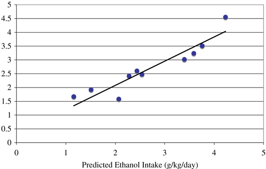Simple regression of observed versus predicted daily ethanol intake (g/kg) for the 12 months of ethanol self-administration (R = 0.94, r ² = 0.88; F(1,8) = 56.6, p = 6.8 × 10⁻⁵).

Fig. 2.

Representative cumulative records of ethanol intake (4% w/v, ml) over session time in 4 consecutive days depicting an extended alcoholic “spree” as defined by a session intake of >4/0 g/kg ethanol. (A) Records from monkey 6893 (4.9 kg body weight) and (B) records from monkey 6888 (6.56 kg body weight); both monkeys were classified as heavy drinkers (see methods). The lights were off in the room between session hours 7 to 20 (6:00 PM to 7:00 AM). For comparison, average daily intake for monkey 6893 was 3.58g/kg (439 ml) and for monkey 6888 was 4.20 g/kg (688 ml) over the 12 months of ethanol access.

There are striking similarities and some important differences in these self-administration patterns. First, Fig. 2A shows that monkey 6893 nearly reached the criteria for a spree day on January 16 with an intake of 3.94 g/kg (a 16 drink equivalent). On the next 3 consecutive days, January 17, 18, Jan 19, the monkey self-administered 6.44 g/kg (a 26 drink equivalent), 5.92 g/kg, and 4.63 g/kg, respectively. These across-day intakes show little perturbation to the daily pattern of ethanol self-administration. Specifically, the size of the first ethanol bout, within the first 15 minutes of the session, and the final ethanol bout the next morning nearly account for the above average ethanol intakes in this monkey. In contrast, Fig. 2B shows that monkey 6888 had began a 2-day spree on January 16 (4.7 g/kg, 19 drink equivalent) and January 17 (5.45 g/kg, 22 drink equivalent) followed by a session of relatively low total intake (1.60 g/kg) and very little ethanol self-administration after the third hour of the session. On the following day (January 19), the monkey did not begin drinking ethanol substantially until after the fourth hour of the session, taking essentially a 24 hour break from his normal heavy intake pattern. After this self-imposed abstinence, however, the monkey engages in the largest ethanol bout of the 4 consecutive days (4.5 hours on January 19) and finishes the session with another intake of 4.26 g/kg. Figure 2 also shows notable features of drinking ethanol throughout the night, with only several hours between drinks of alcohol, and drinking ethanol when the room lights are turned on at 7:00 am. Drinking through the night and during the morning hours is a common feature of monkeys that self-administer more than 3.0 g/kg ethanol per day (i.e., a heavy drinking monkey; Vivian et al., 2001; Grant and Bennett, 2003).

Therefore, the classification of 3.0 g/kg/day captures a heavy drinking phenotype and this single variable was used to search for predictors based on FPCA. Summarized daily measures during induction that were subjected to the PCA for PCRA are listed in Table 3 (with additional data for water, 0.5 and 1.0 g/kg inductions phases available upon request). PCRA showed that only drinking behavior during the induction of 1.5 g/kg ethanol per day for 30 sessions, and not drinking behavior during induction of 0.5 g/kg ethanol or 1.0 g/kg ethanol, was predictive. Thus, only the summary data for the 1.5 g/kg induction dose is shown (Table 3). PCA results of the 12 predictors for this induction dose showed that the first 5 principal components with the highest predictions were number of ethanol bouts, largest ethanol bout volume, percentage of the 1.5 g/kg dose taken in the largest bout, water intake during the rest of the day, the number of pellets delivered in State 1 (under the FT 5 minutes schedule) (see last row, Table 3). These 5 components accounted for over 96% of the total variation. Any of the other 12 predictors accounted individually for less than 2%of the total variation. The first 5 components were, therefore, used for further regression analysis.

During stepwise model selection, only the first principal component entered the final model. Collectively, the model, based on these 5 components, can be summarized as “quantity/frequency/speed of drinking.” This component accounted for 43.4% of total variation in the predictor and showed a high positive correlation with the largest bout volume (0.91), the percentage of the 1.5 g/kg ethanol dose consumed in the largest bout of each induction session (0.91), the percentage of fixed intervals during induction where drinking occurred (0.79) and water intake during the rest of the day (0.84). High negative correlations of this component of “quantity/frequency/speed of drinking” were found with the number of pellets delivered during state 1 (−0.90), and the total number of ethanol bouts (−0.88). Thus, a drinking typography of rapidly drinking large volumes of ethanol (i.e., gulping) in fewer bouts during the induction of 1.5 g/kg ethanol was consistently associated with eventually becoming a heavy drinker. The loading structure of this component is shown at the bottom of Table 3. The data were placed back into the PCRA model and computed for “predicted” amount of ethanol consumed over the 12 months of 22 hour ethanol self-administration (Table 4). The correlation between predicted and actual was very strong [R = 0.94, r² = 0.88; F(1,8) = 56.6, p = 6.8 × 10⁻⁵], high-lighting the strength of the data and the analysis approach used here.

Classification based on FPCA was performed for each predictor at each induced dose. We did leave-one-out cross-validation classification to search for the “best” FPC, (i.e., giving the lowest error rate). For the percentage of the 1.5 g/kg ethanol dose consumed in the largest bout, the “best” PC turned out to be the first PC (resembling the mean curve of the 10 monkeys as shown in Fig. 8). Largest ethanol bout volume, percentage of fixed intervals in which there was a drinking record, and total pellets delivered in state 1 (i.e., under the FT 5 minutes schedule) classify a heavy drinker equally well, as using the percentage of the 1.5 g/kg dose consumed in the largest bout. All these predictors results in 1 (out of 10) mis-classification (results not shown). We highlight the variable “percentage of 1.5 g/kg dose in a single bout,” rather than “largest ethanol bout volume,” because the percentage of dose variable equates volume across monkeys of different weights, and therefore different volumes required to achieve the same dose.

Fig. 8.

(A) Covariance surface of the percentage of ethanol taken in the largest single bout over the 30 days of 1.5 g/kg exposure, from which FPCs are decomposed. The diagonal of the surface (right side graph) shows the variances at different days and off-diagonal shows the covariances among different days (left side graph). Largest bout percentage differed the most at 3 time periods (see text); (B) The percentage of ethanol taken in the largest single bout over 30 days of 1.5g/kg exposure overlaid with smoothed curves. Stars represent the observed individual daily measure and the curves are the estimated level based on FPCA.

Examples of drinking large volumes in bouts (gulping) during the induction of water and the induction of 1.5 g/kg dose of ethanol for an eventual heavy drinker (monkey 6887) and an eventual nonheavy drinker (6895) are shown in Fig. 3. This figure compares the final day of being induced to drink water (induction day 30) with that of 1.5 g/kg ethanol (induction day 120). The cumulative recordings of drinking water as a function of session time shows that monkey 6895 was induced to drink water as rapidly as monkey 6887. In contrast to water, monkey 6895 required almost 3 hours to drink the 1.5 g/kg ethanol dose. During the session depicted, the monkey “sips” his drinks and his largest ethanol bout was 67 ml (from 15 to 57 minutes), accounting for only 35% of the total dose. In comparison, monkey 6887 drank water and 100% of the 1.5 g/kg dose of ethanol in a topology dominated by rapid drinking and finishing the entire 219 ml in a single bout. The highly negative index of curvatures (IOC; Fry et al., 1960) describes a negative acceleration of drinking within the interval of pellet delivery (faster drinking at the beginning of an interval when the pellet is delivered; see also Fig. 5) by both monkeys for both fluids. This pattern is indicative of strong schedule control over drinking for both monkeys. Thus, the difference between the monkeys in drinking typology towards ethanol is not due to the effectiveness of the schedule to generate SIP, but whether the monkey increased the volume of each bout (sips vs. gulps) of ethanol. It is this aspect of intake that was predictive of future classification as a heavy drinker.

Fig. 3.

Representative drinking patterns depicting the typology of “gulping” versus “sipping” during the induction of water or 1.5 g/kg ethanol. Shown are the final induction session of water (blue) or 1.5g/kg ethanol (red) for monkeys 6887 (an eventual heavy drinker) and 6895 (an eventual nonheavy drinker). Both monkeys drank water in a single bout (<5-minute break in continuous drinking) and within the first 25 minutes of the session onset, but differed substantially in their ability to rapidly drink 1.5 g/kg ethanol. Monkey 6887 drank 1.5 g/kg ethanol in a single bout and finished within 35 minutes of session onset. The highly negative index of curvature (IOC) (−0.75 and −0.58) indicates that drinking occurred after pellet delivery and was followed by a short pause of 1 to 2 minutes before the next pellet (interval). In contrast, monkey 6895 required almost 3 hours to drink 1.5 g/kg ethanol. His largest ethanol bout was 67 ml (encircled and occurring from 15 to 57 minutes in the session) and accounted for only 35% of the total dose. The monkey only drank in 68% of the pellet intervals, although the IOC (−0.47) suggests that the drinking, when it occurred, was related to pellet delivery.

Fig. 5.

(A) BEC (mg/dl) taken 90 minutes after the onset of the session is highly correlated with the percentage of 1.5 g/kg induced dose that is taken in the largest bout of the session (r² = 0.46; p < 0.001, n = 58). All monkeys had 6 samples 5 days apart, except 6889, which had 4 samples. (B) Series of 4 cumulative records of drinking during the induction of ethanol self-administration for monkey 6887 (an eventual heavy drinker) corresponding to session where BEC was taken. Shown are the June 5, 16, 20, and 25 drinking patterns where the percentage of the 1.5 g/kg dose taken in the largest bout was 37%, 43%, 70%, and 85%, respectively. Vertical grid lines correspond to pellet delivery and drinking is highly related to pellet delivery. The figure illustrates the challenge to the monkey to rapidly gulp the 1.5 g/kg dose and the gradual increase in volume (bout size) over sessions.

During the induction phase, BECs taken every fifth session at 30, 60, and 90 minutes into the 0.5, 1.0, and 1.5 g/kg sessions, respectively, were directly related to the amount of ethanol consumed (Fig. 4A and 4B). Correlations between intake at the time of the samples and BEC were highly correlated in the entire group of monkeys (R = 0.93, p < 0.001), as well as analyzed separately for the eventual heavy drinkers (R = 0.93, p < 0.001) and eventual nonheavy drinkers (R = 0.92, p < 0.001). However, a major difference between monkeys that were eventually classified as heavy or nonheavy is that all the eventual heavy drinkers, compared to only 2 of the nonheavy drinkers, finished the 1.5 g/kg induction dose in a 90 minute period (when blood samples were drawn for BEC analysis). Indeed, the clustering of BEC under 0.5, 1.0, and 1.5 g/kg in the eventual heavy drinkers (Fig. 4B) shows that this group of monkeys most commonly finished the induced dose by the time the blood sample for BEC analysis was drawn. In contrast, the eventual nonheavy drinkers have a range of intakes (up to and including the induced dose limit) when blood was drawn.

Fig. 4.

Blood ethanol concentrations (BEC, mean ± SD) for each monkey taken and induced dose (n = 6 samples/monkey/induced dose). Blood samples were taken every fifth day of ethanol induction following 30, 60, and 90 minutes after the start of the session to induce the consumption of 0.5, 1.0, and 1.5 g/kg sessions (see Materials and Methods). The x-axis shows the actual amount of ethanol consumed when the blood sample was taken. The top graph depicts the BECs for the eventual nonheavy drinkers and the bottom graph shows the BECs for the eventual heavy drinkers. Actual intakes and measured BEC were highly correlated in eventual nonheavy and eventual heavy drinkers (r² = 0.85, 0.86, respectively; p < 0.0001). Compared to the nonheavy drinkers, the heavy drinkers had significantly higher average BEC in induction only during the 1.5 g/kg induction dose of ethanol (see Results).

BECs taken at 30 minute after the start of the 0.5 g/kg induction sessions averaged (±SEM) 27 ± 3 and 19 ± 4 mg/dl in the eventual heavy (n = 4 monkeys, 24 total samples) and nonheavy (n = 6 monkeys, 36 total samples) drinking monkeys, respectively. The average (±SEM) BEC taken 60 minutes after the start of the 1.0 g/kg induction sessions was 65 ± 18 mg/dl (n = 24 total samples) in the eventual heavy drinkers and 57 ± 9 mg/dl (n = 36 total samples) in the eventual nonheavy drinkers, levels that were not statistically different from each other. However, 90 minute following the start of the 1.5 g/kg ethanol inductions sessions, there was a significant difference (p < 0.01) in the average BEC between the eventual heavy drinkers (113 ± 15 mg/dl, n = 22 total samples) from the average BEC of the nonheavy drinkers (84 ± 12 mg/dl, n = 36 total samples). These data suggest that the induction schedule was equally effective in elevating postingestion BECs up until the 1.5 g/kg induction dose. Even though the average BECs following the 1.5 g/kg dose was different between eventual heavy and nonheavy drinkers, this variable was not the strongest predictor of future ethanol self-administration based on the FPCA.

Figure 5, Figure 6, Figure 7, and Figure 8 show only the results from the percentage of the 1.5 g/kg ethanol dose consumed in the largest bout over the 30 induction sessions (also labeled “% of 1.5 g/kg ethanol dose taken in the largest bout” in Fig. 5 and Table 3). Figure 5A illustrates that this variable was highly correlated with BEC during the induction of 1.5 g/kg (R = 0.68, p < 0.001; Fig. 5A). Although the correlation is not as strong as BEC and actual intake (see Fig. 4), it is notable that a drinking typology is highly correlated with BEC. Thus, “gulping” rather than “sipping” typologies of drinking a 1.5 g/kg dose had the functional consequence of resulting in elevated BECs above the 80 mg/dl legal limit in the United States (Fig. 5A). However, the drinking typology of gulping large doses was not a static characteristic of an animal, as shown in Fig. 5B. This shows that monkey 6887 (an eventual heavy drinker) required approximately 20 sessions to regain the pattern of gulping under the induction schedule when the dose of ethanol was increased to 1.5 g/kg dose (Fig. 6 shows that the monkey finished the last 6 sessions of 1.0 g/kg ethanol in a single bout). Thus, the within-subject dynamics of drinking 1.5 g/kg reflects the initial challenges (even to an eventual heavy drinker) of repeatedly drinking a clearly intoxicating dose of ethanol. Figure 5B also shows the clear relationship between pellet delivery (vertical lines at 5 minutes intervals) and drinking. As indicated by the negative IOC values (Table 3), drinking occurred immediately after pellet delivery. Drinking also occurred in a high percentage of the 5 minute FT intervals during induction (83%, 83%, 87%, and 53% for June 5, 16, 20, and 25, respectively; see also Fig. 3 and Table 3). Both IOC and the percentage of intervals with drinking reflect the adjunctive nature of schedule-induced drinking.

Fig. 6.

The percentage of the required induction volume taken in the largest bout of each session for water induction (sessions 1–30), 0.5 g/kg ethanol induction (sessions 31–60), 1.0 g/kg ethanol induction (sessions 61–90), and 1.5 g/kg ethanol (sessions 91–120). The top 4 graphs (A) depict the eventual heavy drinkers and the bottom 6 graphs (B) depict the eventual nonheavy drinkers. The volume of water was equal to the volume of 1.5 g/kg ethanol (4% w/v) and all monkeys but 6886 drank water in a single bout in at least 50% of the sessions.

Fig. 7.

The number of induction sessions where the volume of the induced dose was consumed in a single bout. Data are a summary of the graphs in Fig. 5 for the induction doses of 0.5, 1.0, and 1.5 g/kg. Monkeys are rank-ordered (left to right) on their eventual average ethanol intakes (g/kg/d; given in Table 4) during the 12 months of ethanol self-administration following induction. The graph illustrates that eventual heavy drinkers and nondrinkers could not be distinguished with this measure in the 30 sessions of 0.5 g/kg ethanol induction and are easily distinguished with this measure in the 30 sessions of 1.5 g/kg ethanol induction.

Figure 6 shows the percentage of induction volume consumed in the largest bout for each session of water, 0.5, 1.0, and 1.5 g/kg. It is clear from Fig. 6 that all monkeys, with the exception of monkey 6886, could ingest large volumes of water under the induction conditions, accounting for 90 to 100% of required fluid intake in their largest bout in well over half their inductions sessions. Indeed, half of the monkeys (6888, 6889, 6894, 6892, 6896) were induced to drink their entire water “dose” in a single bout nearly exclusively. As in Fig. 3, these data show that the ability to rapidly ingest water under induction conditions does not necessarily transfer to the rapid intake of ethanol. Indeed, the 1.0 and 1.5 g/kg doses were challenging to all monkeys in terms of large intakes within a bout. The fluctuations between sipping and gulping depicted in Fig. 5B (for a single monkey) are reflected in Fig. 6 for all monkeys albeit at different induction doses. Indeed, 2 monkeys (6888 and 6889) that were eventual heavy drinkers show a delayed disruption of gulping 1.5 g/kg dose in a single bout and the other 2 monkeys (6887 and 6893), show an initial sipping pattern with an eventual return to drinking the gulping the 1.5 g/kg dose in a single bout.

Summary data highlighting the main finding of drinking the induced dose in the largest bout for the 90 ethanol-induction sessions is shown in Fig. 7. In this graph, the number of sessions (out of 30 sessions) in which the entire dose is consumed in a single bout (i.e., the number of sessions at 100% in Fig. 6), is given for each monkey and induction dose. The monkeys are categorized as eventual heavy drinkers or eventual nonheavy drinkers and listed from left to right in decreasing order of average daily ethanol intake during the 12 months of ethanol self-administration (means given in Table 3). Figure 7 illustrates the emergence of this variable as a significant distinguishing variable for heavy versus nonheavy status. Specifically, the number of 0.5 g/kg induction sessions where the 0.5 g/kg dose was taken in a single bout did not show a group difference. A difference emerged with the 1.0 g/kg induction dose, in which heavy drinkers consumed the 1.0 g/kg dose in a single bout in at least 50% (15) of the sessions whereas the nonheavy drinkers consumed the 1.0 g/kg dose in less then 37% (11) of the sessions. Finally, all the eventual nonheavy drinkers (bottom 6 graphs of Fig. 6) had either zero (monkeys 6886, 6891, and 6896) or a single session (monkeys 6894, 6892, 6895) in which the entire volume was taken in a single bout (Fig. 7).

Figure 8A illustrates the temporal fluctuations and covariance of largest bout percentage over the 30 days (days 90 to 120) of induction for the 10 monkeys. This Figure essentially collapses the 1.5 g/kg data shown in red in Fig. 6 across all subjects. Diagonal of the surface shows the variances at different days and off-diagonal shows the covariance among different days (Fig. 8A, left panel). Largest bout percentage for the 10 monkeys were quite close at the beginning of the 1.5 g/kg ethanol dose, then started to vary, reaching the peak variation around day 97. The second wave of variation peaked at day 110 (Fig. 8A right panel). The actual percentage of ethanol taken in the largest single bout over 30 days of 1.5g/kg exposure is shown in Fig. 8B (blue stars) overlaid with the smoothed curves (red lines) that are the estimated bout intakes based on FPCA.

DISCUSSION

The major finding of the present study is the ability to predict future levels of chronic ethanol self-administration from drinking typographies that emerge early in the initiation of ethanol drinking. This typography encompassed large volumes consumed in bouts (less than a 5 minute lapse between fluid intake), coined gulping. Specifically, the behavioral data show that the ability to rapidly and repeatedly drink a 1.5 g/kg dose of ethanol, roughly drinking the equivalent in alcohol content to 6 drinks in a 70 kg person without a 5 minute break, was highly predictive of the future classification as a “heavy” drinker. The definition of a heavy drinker was an average daily intake of >3.0 g/kg ethanol, and this encompassed 4 of the 10 monkeys, a similar proportion (40%) of heavy drinking monkeys to our previous findings in this species (Vivian et al., 2001), Further, there was a wide (>3-fold) and normal distribution of the 12-month total and average ethanol intakes. The heavy drinkers frequently (over 20% of total session) engaged in consecutive days of “spree” or “bender” drinking defined as daily intakes over 4.0 g/kg ethanol. Spree drinking was virtually absent from the drinking patterns of all nonheavy drinking monkeys (Fig. 1B). This term “spree” is based on reports that alcoholics will “spree-drink” 16 to 26 alcoholic drinks in at least 16 of 20 consecutive days where alcohol was freely available to them (Mello and Mendelson, 1970; see also Nathan et al., 1971). Indeed, it is rather striking to sprees in alcoholics drinking on an experimental ward (Mello and Mendelson, 1971; Nathan et al., 1971) that closely resemble the day-to-day patterns of total intake and within session intakes in the monkeys (Fig. 2). The data suggest that establishing a pattern of gulping large volumes of alcohol early in one’s drinking history places an individual at risk for future alcohol consumption indicative of an alcoholic drinking phenotype.

Although interval schedules can reliably induce adjunctive drinking, scheduled-induced polydipsia is not a fixed or reflexive behavior. Indeed, the data shown here illustrate that although 90% of all monkeys (eventual heavy and nonheavy drinkers) demonstrated scheduled-induced gulping of water, only a smaller portion of the monkeys increased their volume per bout (gulping) of ethanol. The cumulative records in Fig. 3 were chosen to illustrate that monkeys which gulp their water are not necessarily also going to gulp their alcohol. The capacity to rapidly drink a 6-drink equivalent of alcohol is an important individual difference that distinguishes between heavy and nonheavy drinkers, whereas rapidly drinking water does not predict future alcohol drinking. Thus, alcohol-naive drinking typologies are not predictive of future ethanol intakes and exposure to alcohol, indeed fairly high doses of ethanol, is necessary if the goal of an experiment is to investigate risk for heavy drinking in primates. If, however, the goal is to look for protective mechanisms, it should be noted that monkey 6886 was the only consistent “sipper” of water, was never induced to gulp any dose of ethanol, and was an eventual nonheavy drinker.

The study design incorporated the 30-session epochs of schedule-induction at each dose to allow the monkeys multiple opportunities to associate drinking ethanol with its intoxicating effects. Further, the induction schedule maintained ethanol consumption in all monkeys until the 0.5, 1.0 or 1.5 g/kg intakes were entirely consumed within a session and, perhaps most importantly, induced these intakes across consecutive daily sessions (Fig. 5B). The session-to-session drinking patterns during induction (Fig. 5B and Fig 6) show individual differences in disruptions of rapid ethanol intakes. For example, some monkeys were sensitive to the disrupting effects of fairly low doses of ethanol (0.5 g/kg) and did not resume the gulping pattern they displayed for water (e.g., monkeys 6895), while other monkeys were disrupted by the same dose and regained the gulping pattern (e.g., monkey 6889). The separation of monkeys that were differentially sensitive to the effects of ethanol on intake patterns is also illustrated in Fig. 7, where the number of session in which the induced dose was consumed in a single bout steadily decreased in all monkeys as the induced dose increased. Overall, the eventual nonheavy drinkers show disruptions in the pattern of gulping beginning at 0.5 g/kg (monkeys 6895, 6896) and 1.0 g/kg doses (monkeys 6891, 6892, 6894). In contrast, the eventual heavy drinkers required the induction dose of 1.5 g/kg ethanol before intake patterns were disrupted in at least 50% of the session. The apparent tolerance to the disrupting effects of ethanol on drinking typology may underlie the eventual ability to repeatedly self-administer very high doses of ethanol associated with heavy drinking and alcoholic sprees.

Self-intoxication with ethanol in this study was measured by BECs. Specifically, “gulping” the 1.5 g/kg dose of ethanol under the induction schedule led to BECs consistently over 80 mg/dl, whereas “sipping” this dose resulted in BECs under 80 mg/dl (Fig. 4 and Fig 5A). Because 9 out of 10 monkeys showed that they could regularly gulp water, the monkeys which became “ethanol sippers” appear to have adjusted their drinking under the induction schedule to avoid intoxication (Fig. 7). Of particular interest is the pattern of the eventual lowest drinker (6896), which drank in a very stable, but low-bout volume, manner across the 30 sessions of 1.5 g/kg ethanol induction. These data suggest that the monkey was titrating his ethanol consumption to avoid elevated BECs (actual range was 56 to 77 mg% during 1.5 g/kg induction). The data further suggest that the monkeys whose ability to gulp a larger dose of ethanol (i.e., 1.5 g/kg vs. 1.0 g/kg), was disrupted, but regained, over the course of the 30 sessions were also subjecting themselves to higher BECs. Perhaps the analysis of “quantity/frequency/speed” of drinking was not predictive when 0.5 or 1.0 g/kg ethanol was induced because the intoxicating effects of ethanol at these lower doses was not enough to identify individuals that would repeatedly engage in self-intoxication at levels above 80 mg/dl, and this is a critical threshold in continuing on to be a heavy drinker. In fact, the BECs were not different between eventual heavy and nonheavy drinkers until the 1.5 g/kg induction dose. These parameters appear to be consistent with the monkeys associating gulping alcohol with intoxication.

One of the criticisms leveled at using scheduled-induced polydipsia to establish ethanol self-administration has been that the consumption of ethanol falls to low levels when the induction schedule is suspended (see Falk, 1998; Samson and Chappell, 2003). This is clearly not the case in the present use of this procedure (Fig. 1 and Fig 3, Table 4; Vivian et al., 2001). Rather, this monkey model captures a form of heavy drinking that has substantial face validity with human alcoholic drinking. Self-administration in the heavy drinking monkeys given relatively open (22 h/d) access to ethanol results in a high amount of day-to-day variability in the total daily amount of ethanol (Vivian et al., 2001; see also Fig. 2). This variability in daily intakes is very similar to that documented in alcoholics living in an experimental ward and allowed to freely drink alcohol for 18 consecutive days (Nathan et al., 1971). The source of day-to-day variability is under investigation, but may be a response to recent short-term ethanol intakes (e.g., hangovers), cumulative toll of long-term ethanol intakes, disruptions in sleep, provocations with conspecifics, etc. Given this variability, it is remarkable that the PCRA model was able to correctly classify 9 out of the 10 monkeys as chronic binge or nonbinge drinkers and show such a high correlation (R = 0.91) between actual and predicted ethanol intakes over 12 months of daily 22-hour sessions (Table 4). The accuracy of the model may lie in the consecutive patterns of drinking depicted in Fig. 2 showing that ethanol self-administration mostly follows a regular pattern, but with elevated intakes in first bout of the day, increased drinking during the night, and increased morning drinking. The induction schedule appears to have established the behavior of gulping intoxicating amounts of ethanol, and this behavior under unlimited access to ethanol can result in very high intakes.

There has been speculation, and supporting data, in the human subject literature regarding the ability of schedule-induction to increase ethanol consumption specifically by increasing bout size (Doyle and Samson, 1985). Further, it has been suggested that the ability of scheduled induction to increase bout size is a phenomenon that cannot happen in rats, and may be unique to primates (Samson and Chappell, 2003). Our data show that some monkeys increase ethanol bout size whereas others do not. However, monkeys that do engage in a sustained pattern of rapidly drinking large volumes of ethanol during the relatively early stages of ethanol exposure (i.e., during induction) are individuals that subsequently become heavy alcohol drinkers. In at least 1 previous human subjects study, alcoholics were distinguished (a priori) from nonalcoholics in part by gulping their drinks (Nathan et al., 1971). Therefore, the present model of inducing monkeys to drink ethanol in a graded fashion using FT schedules, provides an approach to study individual risk factors for establishing a pattern of alcohol consumption associated with alcohol abuse in human studies. The relationship between baseline hormonal responses (Porcu et al., 2005, Porcu et al. 2006) and the ability to “gulp” a 6-drink equivalent (present data) have yet to be determined; however, it appears that both baseline hormonal responses and acquired drinking typographies contribute to this individual risk.

REFERENCES

- Allen JD, Kenshalo DR. Schedule-induced drinking as a function of interreinforcement interval in the rhesus monkey. J Exp Analysis Behav. 1976;26:257–267. doi: 10.1901/jeab.1976.26-257. [DOI] [PMC free article] [PubMed] [Google Scholar]
- Allen JD, Kenshalo DR. Schedule-induced drinking as functions of interpellet interval and draught size in the Java Macaque. J Exp Analysis Behav. 1978;30:139–151. doi: 10.1901/jeab.1978.30-139. [DOI] [PMC free article] [PubMed] [Google Scholar]
- Byrd LD. Magnitude and duration of the effects of cocaine on conditioned and adjunctive behaviors in the chimpanzee. J Exp Analysis Behav. 1980;33:131–140. doi: 10.1901/jeab.1980.33-131. [DOI] [PMC free article] [PubMed] [Google Scholar]
- Dawson DA. Drinking patterns among individuals with and without DSM-IV alcohol use disorders. J Stud Alcohol. 2000;61:111–120. doi: 10.15288/jsa.2000.61.111. [DOI] [PubMed] [Google Scholar]
- Doyle TF, Samson HH. Schedule-induced drinking in humans: a potential factor in excessive alcohol use. Drug Alcohol Depend. 1985;16:117–132. doi: 10.1016/0376-8716(85)90111-5. [DOI] [PubMed] [Google Scholar]
- Falk JL. Production of polydipsia in normal rats by an intermittent food schedule. Science. 1961;133:195–196. doi: 10.1126/science.133.3447.195. [DOI] [PubMed] [Google Scholar]
- Falk JL. Schedule-induced polydipsia as a function of fixed interval length. J Exp Anal Behav. 1966;9:37–38. doi: 10.1901/jeab.1966.9-37. [DOI] [PMC free article] [PubMed] [Google Scholar]
- Falk JL. The nature and determinants of adjunctive behavior. Physiol Behav. 1971;6:577–588. doi: 10.1016/0031-9384(71)90209-5. [DOI] [PubMed] [Google Scholar]
- Falk JL. Schedule-induced drug self-administration. In: van Haaren F, editor. Methods in Behavioral Pharmacology. Amsterdam, The Netherlands: Elsevier Science; 1993. pp. 301–328. [Google Scholar]
- Falk JL. Drug abuse as an adjunctive behavior. Drug Alcohol Depend. 1998;51:91–98. doi: 10.1016/s0376-8716(98)00084-2. [DOI] [PubMed] [Google Scholar]
- Falk JL, Samson HH, Tang M. Chronic ingestion techniques for the production of physical dependence on ethanol. In: Gross MM, editor. Alcohol Intoxication and Withdrawal. New York: Plenum; 1972. pp. 197–211. [Google Scholar]
- Fry W, Kelleher RT, Cook L. A mathematical index of performance on fixed-interval schedules of reinforcement. J Exp Anal Behav. 1960;3:193–199. doi: 10.1901/jeab.1960.3-193. [DOI] [PMC free article] [PubMed] [Google Scholar]
- Grant KA, Bennett AJ. Advances in nonhuman primate alcohol abuse and alcoholism research. Pharmacol Ther. 2003;100:235–255. doi: 10.1016/j.pharmthera.2003.08.004. [DOI] [PubMed] [Google Scholar]
- Grant BF, Dawson DA, Stinson FS, Chou SP, Dufour MC, Pickering RP. The 12-month prevalence and trends in DSM-IV alcohol abuse and dependence: United States, 1991–1992 and 2001–2002. Drug Alcohol Depend. 2004;74:223–234. doi: 10.1016/j.drugalcdep.2004.02.004. [DOI] [PubMed] [Google Scholar]
- Grant KA, Johanson CE. The nature of the scheduled reinforcer and adjunctive drinking in nondeprived rhesus monkeys. Pharmacol Biochem Behav. 1988;29:295–301. doi: 10.1016/0091-3057(88)90159-1. [DOI] [PubMed] [Google Scholar]
- Green KL, Szeliga KT, Bowen CA, Kautz MA, Azarov AV, Grant KA. Comparison of ethanol metabolism in male and female cynomolgus macaques (Macaca fasicularis) Alcohol Clin Exp Res. 1999;23:611–616. [PubMed] [Google Scholar]
- Gunzerath L, Faden V, Zakhari S, Warren K. National Institute on Alcohol Abuse and Alcoholism report on moderate drinking. Alcohol Clin Exp Res. 2004;28:829–847. doi: 10.1097/01.alc.0000128382.79375.b6. [DOI] [PubMed] [Google Scholar]
- Johnson RA, Wichern DW. Applied Multivariate Statistical Analysis. 4th ed. New York: Prentice-Hall; 1998. [Google Scholar]
- Leng X, Muller HG. Classification using functional data analysis for temporal gene expression data. Bioinformatics. 2006;22:68–76. doi: 10.1093/bioinformatics/bti742. [DOI] [PubMed] [Google Scholar]
- Majchrowicz E. Comparison of ethanol withdrawal syndrome in humans and rats. In: Gross MM, editor. Alcohol Intoxication and Withdrawal. Vol. 3B. New York: Plenum Press; 1977. [DOI] [PubMed] [Google Scholar]
- Majchrowicz E, Mendelson JH. Blood concentrations of acetaldehyde and ethanol in chronic alcoholics. Science. 1970;168:1100–1102. doi: 10.1126/science.168.3935.1100. [DOI] [PubMed] [Google Scholar]
- Meisch RA. Alcohol self-administration by experimental animals. In: Smart RG, Cappell HD, Glaser FB, Israel Y, Kalant H, Popham RE, Schmidt W, Sellers EM, editors. In research advances in alcohol and drug problems. NY: Plenum Press; 1984. pp. 23–45. [Google Scholar]
- Mello NK, Mendelson JH. Experimentally induced intoxication in alcoholics: A comparison between programmed and spontaneous drinking. J Pharmacol Exper Therap. 1970;173:101–116. [PubMed] [Google Scholar]
- Mello NK, Mendelson JH. Drinking patterns during work contingent and non-contingent alcohol acquisition. In: Mello NK, Mendelson JH, editors. Recent Advances in Studies of Alcoholism. Washington, DC: U.S. Gov. Printing Office; 1971. (Pub. No 71-9045) [Google Scholar]
- Mokdad AH, Marks JS, Stroup DF, Gerberding JL. Actual causes of death in the United States. J Am Med Assoc. 2004;291:1238–1245. doi: 10.1001/jama.291.10.1238. [DOI] [PubMed] [Google Scholar]
- Nathan PE, O’Brien JS, Norton D. Comparative studies of the interpersonal and affective behavior of alcoholics and nonalcoholics during prolonged experimental drinking. In: Mello NK, Mendelson JH, editors. Recent Advances in Studies of Alcoholism. Washington, DC: U.S. Gov. Printing Office; 1971. pp. 619–646. (Pub. No 71-9045) [Google Scholar]
- Porcu P, Grant KA, Green HL, Rogers LSM, Morrow AL. Hypothalamic-pituitary-adrenal axis and ethanol modulation of deoxycorticosterone levels in cynomolgus monkeys. Psychopharmcology. 2005;186:293301. doi: 10.1007/s00213-005-0132-2. [DOI] [PubMed] [Google Scholar]
- Porcu P, Rogers LSM, Morrow AL, Grant KA. Plasma pregnenolone levels in cynomolgus monkeys following pharmacological challenges of the hypothalamic-pituitary-adrenal axis. Pharmacol Biochem Behav. 2006;84:618–627. doi: 10.1016/j.pbb.2006.05.004. [DOI] [PubMed] [Google Scholar]
- Porter JH, Kenshalo DR. Schedule-induced drinking following omission of reinforcement in the rhesus monkey. Physiol Behav. 1974;12:1075–1077. doi: 10.1016/0031-9384(74)90158-9. [DOI] [PubMed] [Google Scholar]
- Ramsay JO, Silverman BW. Functional Data Analysis. New York: Springer; 1997. [Google Scholar]
- Rhodes JS, Best K, Belknap JK, Finn DA, Crabbe JC. Evaluation of a simple model of ethanol drinking to intoxication in C57BL/6J mice. Physiol Behav. 2005;84:53–63. doi: 10.1016/j.physbeh.2004.10.007. [DOI] [PubMed] [Google Scholar]
- Samson HH. Initiation of ethanol-maintained behavior: A comparison of animal models and their implication to human drinking. In: Thompson T, Dews PB, Barrett JE, editors. Neurobehavioral Pharmacology. Vol. 6. Hillsdale, NJ: Lawrence Erlbaum Associates; 1987. pp. 221–248. [Google Scholar]
- Samson HH, Chappell A. Failure of a schedule-induction procedure to increase ethanol intake in an established limited-access self-administration condition. Alcohol. 2003;31:161–165. doi: 10.1016/j.alcohol.2003.08.005. [DOI] [PubMed] [Google Scholar]
- Samson HH, Falk JL. Pattern of daily blood ethanol elevation and the development of physical dependence. Pharmacol Biochem Behav. 1975;3:1119–1123. doi: 10.1016/0091-3057(75)90026-x. [DOI] [PubMed] [Google Scholar]
- Sanger DJ. Drug taking as adjunctive behavior. In: Goldberg SR, Stolerman IP, editors. Behavioral Analysis of Drug Dependence. NY: Academic Press; 1986. pp. 123–160. [Google Scholar]
- Schuster CR, Woods JH. Scheduled-induced polydipsia in the monkey. Psychol Rep. 1966;19:823–828. doi: 10.2466/pr0.1966.19.3.823. [DOI] [PubMed] [Google Scholar]
- Shelton KL, Young JE, Grant KA. A multiple schedule model of limited access drinking in the cynomolgus macaque. Behav Pharmacol. 2001;12:559–573. doi: 10.1097/00008877-200112000-00001. [DOI] [PubMed] [Google Scholar]
- Stahre M, Naimi T, Brewer R, Holt J. Measuring average alcohol consumption: the impact of including binge drinks in quantity-frequency calculations. Addiction. 2006;101:756–760. doi: 10.1111/j.1360-0443.2006.01615.x. [DOI] [PubMed] [Google Scholar]
- Vivian JA, Green HL, Young JE, Majerksy LS, Thomas BW, Shively CA, Tobin JR, Nader MA, Grant KA. Induction and maintenance of ethanol self-administration in cynomolgus monkeys (Macaca fascicularis): long-term characterization of sex and individual differences. Alcohol Clin Exp Res. 2001;25:1087–1097. [PubMed] [Google Scholar]