Tertiary and Secondary Structure Elasticity of a Six-Ig Titin Chain

Abstract

The protein titin functions as a mechanical spring conferring passive elasticity to muscle. Force spectroscopy studies have shown that titin exhibits several regimes of elasticity. Disordered segments bring about a soft, entropic spring-type elasticity; secondary structures of titin's immunoglobulin-like (Ig-) and fibronectin type III-like (FN-III) domains provide a stiff elasticity. In this study, we demonstrate a third type of elasticity due to tertiary structure and involving domain-domain interaction and reorganization along the titin chain. Through 870 ns of molecular dynamics simulations involving 29,000–635,000 atom systems, the mechanical properties of a six-Ig domain segment of titin (I65-I70), for which a crystallographic structure is available, are probed. The results reveal a soft tertiary structure elasticity. A remarkably accurate statistical mechanical description for this elasticity is derived and applied. Simulations also studied the stiff, secondary structure elasticity of the I65-I70 chain due to the unraveling of its domains and revealed how force propagates along the chain during the secondary structure elasticity response.

Introduction

Mechanical proteins confer structural support and mechanical compliance upon biological cells and tissues, as evidenced during muscular contraction. The protein titin, which is the largest protein in nature (34,350 amino acids) (1) and composed mainly of immunoglobulin-like (Ig-) or fibronectin-III-like (FN-III) domains (1,2) along with flexible N2B and PEVK (rich in proline, glutamate, valine, and lysine) regions and a catalytic kinase domain (3), provides the passive elasticity required to restore muscle to its resting length after contraction. Through its elasticity, titin also protects muscle fibers from mechanical injury (1,4).

Current understanding of titin's mechanical properties arose from single-molecule force spectroscopy investigations of isolated, native titin as well as recombinant fragments (5–12). From these experiments, a picture began to form describing how titin reacts to mechanical stretching forces: Upon stretching, titin's chain of domains first straightens without unfolding. This is followed by elongation of disordered segments. Finally, at strong forces, the secondary structure of titin's Ig- and FN-III domains unravels, a process referred to as “rupture”. Thus, in addition to the entropic elasticity conferred by the protein's disordered domains, titin's mechanical elasticity can be further classified, as illustrated in Fig. 1, A and B, into two distinct regimes: tertiary structure elasticity (13) due to domain-domain straightening, and secondary structure elasticity (14,15) due to the unraveling of domains.

Figure 1.

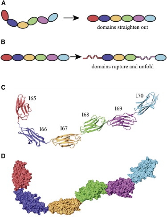
Schematic representation of the soft tertiary structure and stiff secondary structure elasticity for the six-domain titin segment I65-70 (i.e., Ig6). (A) How the arrangement of domains in Ig6 manifests itself in tertiary structure elasticity. (B) How strong forces lead to the rupture of individual domains, an example of secondary structure elasticity. (C) Structure of I65-70 in cartoon representation. The individual domains are color-coded the same way in all subsequent figures. (D) Structure of I65-70 in surface representation; the short linkers among I67-68, I68-69, and I69-70 can be recognized clearly.

Titin's secondary structure elasticity has been extensively characterized through molecular dynamics (MD) and steered molecular dynamics (SMD) simulations that cast light on how the terminal β-strands of its Ig- and FN-III domains stabilize the protein against rupture (16–21). The molecular basis for titin's tertiary structure elasticity, though, is less well characterized—in part due to the lack of atomic resolution structures for multidomain titin constructs, and in part due to the high computational cost associated with performing simulations on large systems involving multiple protein domains. Simulations have been employed to study the tertiary structure elasticity associated with the tandem Z1 and Z2 domains of titin (13). Tertiary structure elasticity was also probed via simulations for relatively short mechanical repeat proteins such as ankyrin (22) and cadherin (23).

The recent availability of the crystal structure of a six-Ig fragment I65-I70 (24) from the I-band of titin offers us an opportunity to computationally study, at atomic resolution, the overall flexibility of titin. Inspection of crystal structure and sequence shows that the linkers between the connected Ig-domains involve long (three-residue length) and short (zero-residue length) links that alternate according to a conserved pattern (24). A schematic for titin I65-I70 (referred to in the following as “Ig6”) is shown in Fig. 1 C. The compact linear arrangements of the Ig-domains connected by short linkers (I67-68, I68-69, and I69-70) can be recognized in the surface representation of Ig6 in Fig. 1 D. Differences in linker lengths have also been observed previously in EM micrographs of titin (24). It remains to be understood, however, how these domain-domain interactions control the overall tertiary structure elasticity of titin.

In this study, we employ MD simulations and statistical mechanical theory to characterize tertiary and secondary structure elasticity of titin Ig6. The free-energy changes associated with bending and twisting motions involving domain pairs were calculated using the adaptive biasing force (ABF) method (25–27). The resulting potentials of mean force were cast into a mathematical description for the force-extension curve characterizing multidomain tertiary structure elasticity. SMD (28) simulations were then carried out to probe the secondary structure elasticity of the entire Ig6 chain by stretching it until all six domains became unfolded. The simulations and theoretical calculations present evidence that the tertiary structure elasticity associated with flexible I-band tandem Ig-domains comprises a soft entropiclike energy barrier to structural deformation, resembling in this respect the elasticity contributed by titin's disordered domains. The simulations also resolve the Ig6 secondary structure elasticity at the atomic level and show how tension among the connected Ig-domains is relieved each time a single domain unfolds.

Methods

Here we describe the molecular models and methods employed in our simulations as well as the statistical mechanical framework for titin's multidomain tertiary structure elasticity. Further details are found in the Supporting Material where the question of timescale adequacy of simulations is discussed (see also Lee et al. (20)).

Simulated systems

Nine systems were investigated. The first four systems involved Ig6 (PDB code 3B43) (24) in ionized water boxes of different sizes: standard equilibration (simEQ); extending Ig6 without unfolding its domains (simEQ-ext and simEXT); fully unfolding all Ig6 domains without disulfide bonds (simEQ-str1 and simSTR1); and fully unfolding Ig6 with disulfide bonds (simEQ-str2 and simSTR2). The final five systems model the individual Ig-pairs from Ig6. The systems are listed in Table 1 and discussed further in the Supporting Material. Altogether, 870 ns of simulations were carried out on systems involving 29,000–635,000 atoms.

Table 1.

Summary of simulations

Name	Structure	Type	Ensemble	Atoms (× 1000)	Size (Å3)	Special parameters	Time (ns)
simEQ	I65-70	EQ	NpT	224	110 × 339 × 63	—	20.0
simEQ-ab	I65-66	EQ	NpT	78	131 × 82 × 77	—	10.0
simEQ-bc	I66-67	EQ	NpT	72	138 × 71 × 77	—	10.0
simEQ-cd	I67-68	EQ	NpT	73	136 × 74 × 77	—	10.0
simEQ-de	I68-69	EQ	NpT	72	129 × 81 × 74	—	10.0
simEQ-ef	I69-70	EQ	NpT	77	131 × 83 × 75	—	10.0
simAB-b	I65-66	ABF	NVT	78	131 × 82 × 77	Bending	25.0
simBC-b	I66-67	ABF	NVT	72	138 × 71 × 77	Bending	27.0
simCD-b	I67-68	ABF	NVT	73	136 × 74 × 77	Bending	50.0
simDE-b	I68-69	ABF	NVT	72	129 × 81 × 74	Bending	44.0
simEF-b	I69-70	ABF	NVT	77	131 × 83 × 75	Bending	41.0
simAB-t	I65-66	ABF	NVT	78	131 × 82 × 77	Twisting	43.0
simBC-t	I66-67	ABF	NVT	72	138 × 71 × 77	Twisting	69.0
simCD-t	I67-68	ABF	NVT	73	136 × 74 × 77	Twisting	79.0
simDE-t	I68-69	ABF	NVT	72	129 × 81 × 74	Twisting	125.0
simEF-t	I69-70	ABF	NVT	77	131 × 83 × 75	Twisting	132.0
simEQ-ext	I65-70	EQ	NpT	227	114 × 353 × 72	∗	5.0
simEXT	I65-70	SCV	NV	277	114 × 353 × 72	10 Å/ns†	10.0
simEQ-str1	I65-70	EQ	NpT	635	2045 × 60 × 53	∗	5.0
simSTR1	I65-70	SCV	NV	635	2045 × 60 × 53	25 Å/ns†	66.0
simEQ-str2	I65-70	EQ	NpT	425	1197 × 64 × 58	∗	5.0
simSTR2	I65-70	SCV	NV	425	1197 × 64 × 58	25 Å/ns†	35.0
sim-RF	I65-70	EQ	NpT	225	430 × 68 × 62	—	18.6
sim-EQ-I65	I65	EQ	NpT	29	75 × 66 × 62	—	18.9

Under the column header “Type”, EQ denotes equilibration, ABF denotes adaptive biasing force simulations, and SCV denotes constant velocity SMD simulations. The “Ensemble” column lists the variables held constant during the simulations; N, V, p, and T correspond to number of atoms, volume, pressure, and temperature, respectively. Footnotes under special parameters describe the motion sampled in the ABF simulation, and, in the case of SMD simulations, which atoms were fixed and the stretching velocity that was employed.

^∗Preequilibrated I65-70 from simEQ resolvated in a large water box to accommodate SMD simulation.

^†α-carbon of N-terminus I65 fixed and force applied to the C-terminus α-carbon of I70.

Molecular dynamics simulations

All MD simulations were performed using NAMD 2.6 (29) and the CHARMM27 (30) force field with CMAP correction (31,32) and TIP3P (33) model for water molecules. The van der Waals interaction cutoff distances were set at 12 Å (the smooth switching function beginning at 10 Å) and long-range electrostatic forces were computed using the particle-mesh Ewald summation method with a grid size of <1 Å, along with the pencil decomposition protocol where applicable. For equilibrium simulations, constant temperature (T = 300 K) was enforced using Langevin dynamics with a damping coefficient of 1 ps⁻¹. In both equilibrium and SMD simulations, constant pressure (p = 1 atm) was enforced through the Nosé-Hoover Langevin piston method with a decay period of 100 fs and a damping time constant of 50 fs.

SMD simulations (28,34,35) fixed the α-carbon at the N-terminus of I65 and applied a force to the α-carbon at the C-terminus of I70. The constant velocity stretching protocol was employed, with stretching velocities of 10 Å/ns in simEXT and 25 Å/ns for simSTR1 and simSTR2. Constant force SMD simulations applied a time-independent potential of V = kd to the specified atom(s), where d is the C_α-C_α distance between the two termini. For the SMD spring constant (36,37), we chose k_s = 3 k_BT/Ų, which corresponds to a root mean-squared deviation (RMSD) value of $\sqrt{k_{\text{B}}T/k_{\mathrm{s}}}\approx 0.6\AA$.

The ABF method (25,26), adapted into NAMD (derived for the NVT ensemble) (27), was employed to calculate the reversible work, or potential of mean force (PMF), for domain-domain hinge-bending and hinge-twisting motions along an a priori selected reaction coordinate. For each Ig-pair, the reaction coordinate was the separation of two centers-of-mass located at the opposing tips of the two Ig-domains corresponding to the N-terminus of one domain and to the C-terminus of the other (for additional detail, see the Supporting Material).

Theory of multidomain tertiary structure elasticity

The springlike behavior of titin's tertiary structure elasticity, which arises before unfolding of secondary structure occurs, comes about from multiple protein domains connected through linkers. Our simulations measured the PMF to open the hinges (connections through the linkers) between adjacent domain pairs. With the PMF, one can describe qualitatively the tertiary structure-based elastic behavior of titin I65-70. For this purpose, we extended the multidomain chain model in Lee et al. (13). A (planar) multidomain chain is depicted in Fig. 2 A, in which, as an example, six domains are connected into a chain, and the overall length of the chain is determined by the five hinge angles (θ_AB to θ_EF). Our ABF calculations treat each Ig pair as an individual unit, uncoupled from its neighbors. For this reason, our model takes the schematic form shown in Fig. 2 B.

Figure 2.

Schematics of the multidomain chain model. (A) The overall length of a six-domain chain is described by five hinge angles. (B) The present multidomain chain model employs a representation in which domain pairs are connected, each domain pair contributing an independent hinge angle not coupled to other domain pairs. This depiction is schematic; every domain contributes only once to the total extension, as seen in panel A.

As shown in Fig. 2 B, a multidomain Ig chain is made of connected domain pairs, each pair j described by a hinge-opening potential function ${\tilde{V}}_{\text{j}}\left({\theta }_{\text{j}}\right)$ determined by the ABF method. The angle dependence of ${\tilde{V}}_{\text{j}}\left({\theta }_{\text{j}}\right)$ is first replaced by a length dependence via the geometric relation

$$x_{\text{j}}\left({\theta }_{\text{j}}\right)=\ell \sin \left({\theta }_{\text{j}}/2\right),$$ (1)

where x_j is the end-to-end distance of the domain pair, θ_j is the hinge angle, and ℓ is the length of the domain pair when it is fully opened (i.e., for θ_j = 180°). In the following, ℓ is set to 90 Å, approximately the end-to-end distance of an open Ig pair. The inverse of Eq. 1 reads θ_j = θ_j(x_j).

Given each PMF, $V_{\text{j}}\left(x_{\text{j}}\right)={\tilde{V}}_{\text{j}}\left({\mathit{\theta }}_{\text{j}}\left(x_{\text{j}}\right)\right)$, the length distribution, p_j(x_j), can be computed via the Boltzmann relation

$$p_{\text{j}}\left(x_{\text{j}}\right)=Z_{\text{j}}^{-1}\exp \left[-V_{\text{j}}\left(x_{\text{j}}\right)/k_{\text{B}}T\right],$$ (2)

where $Z_{\text{j}}={\int }_{-\mathrm{\infty }}^{+\mathrm{\infty }}\exp \left(-V_{\text{j}}\left(x_{\text{j}}\right)/k_{\text{B}}T\right)d{x}_{\text{j}}$ is the partition function.

Because the overall length of the connected chain, X, is the sum of the length of N linker pairs (i.e., $\text{X}={\sum }_{\text{j}=1}^{\text{N}}{x}_{\text{j}}$, illustrated in Fig. 2 B), the overall length distribution of the multidomain chain is

$$P\left(X\right)={\int }_{-\mathrm{\infty }}^{+\mathrm{\infty }}d{x}_1{\int }_{-\mathrm{\infty }}^{+\mathrm{\infty }}d{x}_2\dots {\int }_{-\mathrm{\infty }}^{+\mathrm{\infty }}d{x}_{\text{N}}{p}_1\left(x_1\right)p_2\left(x_2\right)\dots p_{\text{N}}\left(x_{\text{N}}\right)\delta \left(\sum _{\text{j}=1}^{\text{N}}{x}_{\text{j}}-X\right),$$ (3)

which can be expressed (13)

$$P\left(X\right)={\left(2\pi \right)}^{\left(\text{N}-2\right)/2}{\int }_{-\mathrm{\infty }}^{+\mathrm{\infty }}\exp \left[-ikX\right]dk\prod _{\text{j}=1}^{\text{N}}{\tilde{p}}_{\text{j}}\left(k\right),$$ (4)

where ${\tilde{p}}_{\text{j}}\left(k\right)$ is the Fourier transform of p_j(x_j), namely,

$${\tilde{p}}_{\text{j}}\left(k\right)={\left(2\pi \right)}^{-1/2}{\int }_{-\mathrm{\infty }}^{+\mathrm{\infty }}{p}_{\text{j}}\left(x_{\text{j}}\right)\exp \left[ik{x}_{\text{j}}\right]d{x}_{\text{j}}\text{.}$$

To compute P(X) using Eq. 4, p_j(x_j) needs to be extracted first from ABF data. For this purpose, the ABF data are fitted to a simple mathematical expression for p_j(x_j), such that taking the Fourier transform of p_j(x_j) and the subsequent integration (Eq. 4) are feasible. We choose to employ a sum of two Gaussians, nonvanishing only for x_{j, min} ≤ x_j ≤ x_{j, max}, namely

$$p_{\text{j}}\left(x_{\text{j}}\right)=a_1\exp \left[-c_1{\left(x_{\text{j}}-b_1\right)}^2\right]+a_2\exp \left[-c_2{\left(x_{\text{j}}-b_2\right)}^2\right],$$ (5)

with parameters a₁, b₁, c₁, a₂, b₂, and c₂, and x_{j, min}, x_{j, max} fitted to ABF data (see Results).

The central limit theorem (38) states that for large N, P(X) assumes the form of a Gaussian with average $\overline{X}$ and mean-square deviation Σ², i.e.,

$$P\left(X\right)={\left(2\pi {\Sigma }^2\right)}^{-1/2}\exp \left[-{\left(X-\overline{X}\right)}^2/2{\Sigma }^2\right]\text{.}$$ (6)

Here $\overline{X}$ is the sum of the averages of $x_{\text{j}}\left(\overline{X}={\sum }_{\text{j}=1}^{\text{N}}{\overline{x}}_{\text{j}}\right)$ and Σ² the sum of the mean-square deviations σ_j² of p_j(x_j) $\left({\sum }^2={\sum }_{\text{j}=1}^{\text{N}}{\sigma }_{\text{j}}^2\right)$.

So far we have considered the length distribution of a multidomain chain without external force. However, of interest is how the length changes when a (constant) force f is applied. The potential for the bending motion of each hinge j is then

$${\widehat{V}}_{\text{j}}\left(x_{\text{j}}\right)=V_{\text{j}}\left(x_{\text{j}}\right)-f{x}_{\text{j}}\text{.}$$ (7)

As a consequence, the length distribution of each domain pair, ${\widehat{p}}_{\text{j}}\left(x_{\text{j}}\right)$, becomes

$${\widehat{p}}_{\text{j}}\left(x_{\text{j}}\right)=\exp \left[-{\widehat{V}}_{\text{j}}\left(x_{\text{j}}\right)/k_{\text{B}}T\right]/{\int }_{-\mathrm{\infty }}^{+\mathrm{\infty }}\exp \left[-{\widehat{V}}_{\text{j}}\left(x_{\text{j}}\right)/k_{\text{B}}T\right]d{x}_{\text{j}}\text{.}$$ (8)

The value ${\widehat{p}}_{\text{j}}\left(x_{\text{j}}\right)$ allows one to determine the average domain pair-length ${\langle x_{\text{j}}\rangle }_{{\widehat{V}}_{\text{j}}}$ (the subscript denotes that the average is performed over all configurations weighted by the Boltzmann factor corresponding to ${\widehat{V}}_{\text{j}}$)

$${\langle x_{\text{j}}\rangle }_{{\widehat{V}}_{\text{j}}}={\int }_{-\mathrm{\infty }}^{+\mathrm{\infty }}{x}_{\text{j}}{\widehat{p}}_{\text{j}}\left(x_{\text{j}}\right)d{x}_{\text{j}}={\int }_{-\mathrm{\infty }}^{+\mathrm{\infty }}{x}_{\text{j}}\exp \left[-{\widehat{V}}_{\text{j}}\left(x_{\text{j}}\right)/k_{\text{B}}T\right]d{x}_{\text{j}}/{\int }_{-\mathrm{\infty }}^{+\mathrm{\infty }}\exp \left[-{\widehat{V}}_{\text{j}}\left(x_{\text{j}}\right)/k_{\text{B}}T\right]d{x}_{\text{j}}\text{.}$$ (9)

One can derive (see the Supporting Material)

$${\langle x_{\text{j}}\rangle }_{{\widehat{V}}_{\text{j}}}={\langle x_{\text{j}}\exp \left[f{x}_{\text{j}}/k_{\text{B}}T\right]\rangle }_{V_{\text{j}}}/{\langle \exp \left[f{x}_{\text{j}}/k_{\text{B}}T\right]\rangle }_{V_{\text{j}}}\text{.}$$ (10)

The average overall end-to-end distance, $\langle X\rangle ={\sum }_{\text{j}=1}^{\text{N}}{\langle x_{\text{j}}\rangle }_{{\widehat{V}}_{\text{j}}}$, can then be written

$$\langle X\rangle =\sum _{\text{j}=1}^{\text{N}}\left[{\langle x_{\text{j}}\exp \left[f{x}_{\text{j}}/k_{\text{B}}T\right]\rangle }_{V_{\text{j}}}/{\langle \exp \left[f{x}_{\text{j}}/k_{\text{B}}T\right]\rangle }_{V_{\text{j}}}\right]\equiv g\left(f\right)\text{.}$$ (11)

From this one obtains the force-extension curve f = g⁻¹(〈X〉), which is well-defined as g is a monotonic function of f as shown in the Supporting Material.

In the case where the applied force, f, is small, Taylor expansion of the exponential terms in Eq. 11 yields

$$\langle X\rangle \approx \sum _{\text{j}=1}^{\text{N}}\left[{\langle x_{\text{j}}\rangle }_{V_{\text{j}}}+\left(f/k_{\text{B}}T\right){\mathit{\sigma }}_{\text{j}}^2\right]=\overline{X}+\left(f/k_{\text{B}}T\right)\sum _{\text{j}=1}^{\text{N}}{\mathit{\sigma }}_{\text{j}}^2,$$ (12)

where σ_j² is the mean-square deviation of the length distribution p_j(x_j) and $\overline{X}$ is defined as ${\sum }_{\text{j}=1}^{\text{N}}{\langle x_{\text{j}}\rangle }_{V_{\text{j}}}$. It is then obvious that the chain behaves as a spring of resting length $\overline{X}$ and overall spring constant

$$k_{\text{chain}}=k_{\text{B}}T/\sum _{\text{j}=1}^{\text{N}}{\sigma }_{\text{j}}^2\text{.}$$ (13)

This behavior is the one that also characterizes the statistical mechanics of the potential in Eq. 6. Equations 12 and 13 hold only for small forces, i.e., for f_x << k_BT; in general, one needs to use Eq. 11.

Results

Equilibration of titin I65-70 reveals interdomain flexibility

The crystal structure for titin I65-70 was solvated in a water box under physiological ionic conditions and free dynamics were performed for 20 ns in simEQ (see Table 1). Analysis of the RMSD of the protein revealed that the individual domains of titin Ig6 remained stable. The bending and twisting angles between Ig-domains along the crescent-shaped chain were observed to fluctuate during relaxation, suggesting that such interdomain motions represent a source of elasticity. Equilibrium simulations alone, however, are not sufficient to quantitatively describe this elasticity. We employed a combination of SMD and ABF simulations to fully characterize the underlying energetics of this interdomain-based, so-called tertiary structure elasticity.

Overall tertiary structure elasticity of titin Ig6

To assess the soft elasticity arising upon extending Ig6 from a crescent-shaped chain to a linear chain, SMD simulations were carried out as described below (see also the Supporting Material). Such simulations (35) had successfully characterized the elasticity of titin I91 (7,17), fibronectin (18), ankyrin (22), and cadherin (23). In simEXT, the equilibrated Ig6 structure from simEQ had its N-terminus α-carbon fixed while a force was applied to the C-terminus α-carbon at a stretching velocity of 10 Å/ns. The direction of stretching was chosen to lengthen the Ig6 chain, and force was applied until the chain was completely straightened, but with avoiding secondary structure disruption. The structural transition is illustrated in Fig. 3 A. The extension versus time, x(t), curve is provided in Fig. S4 in the Supporting Material. The value x(t) is governed by the Langevin equation in the strong friction limit, which can be written

$$\gamma \dot{x}=f_{\text{chain}}\left(x\right)-k_{\text{s}}\left(x-vt\right)+\sigma \xi \left(t\right),$$ (14)

where f_chain(x) is the force due to the tertiary elasticity of the Ig6 chain, k_s is the SMD spring constant (k_s = 3 k_BT/Ų; see Methods), v is the stretching velocity (v = 10 Å/ns), and the last term describes (thermal) Gaussian white noise with RMSD denoted by σ and 〈ξ(t)〉 = 0. According to the fluctuation-dissipation theorem, it holds that σ² = 2 k_BTγ. As long as f_chain(x) is negligible compared to $\gamma \dot{x}$ (i.e., for $\left|f_{\text{chain}}\left(x\right)\right|\ll \left|\gamma \dot{x}\right|$), one can write for the average extension, 〈x(t)〉,

$$\gamma \langle \dot{x}\left(t\right)\rangle =-k_{\text{s}}\left[\langle x\left(t\right)\rangle -vt\right],$$ (15)

the solution of which is

$$\langle x\left(t\right)\rangle =vt-\left(v\gamma /k_{\text{s}}\right)\left[1-\exp \left(-k_{\text{s}}t/\gamma \right)\right]\text{.}$$ (16)

Figure 3.

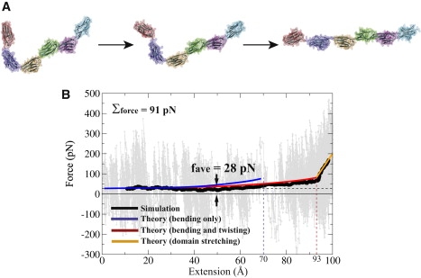
Steered molecular dynamics (SMD) simulations probing the tertiary structure elasticity of titin Ig6. (A) Snapshots from simEXT depicting the extension of Ig6 without unfolding the individual domains. (B) Resulting force-extension curve, with the black trace corresponding to the average force measured. The force fluctuation can be attributed to the SMD spring as discussed in the text. The quantities f_ave and Σ_force, discussed in the text, were computed over the extension range of 10–60 Å, i.e., after the initial relaxation and before the increase of the stretching force above 28 pN (value shown as a black dashed line). The blue and red traces were computed by using the multidomain chain model to determine f_chain(x) and solving Eq. 17 as described in the text, with the blue trace computed by considering only the hinge-bending motions, and the red trace considering both the bending and twisting motions. The orange trace describes the last ∼10 Å of Ig6 extension stemming from the intrinsic stretching of the individual domains; the elasticity characterizing this motion was measured from an equilibrium simulation described in the text and in the Supporting Material. The agreement between simulation (black) and theoretical description (red, orange) does not involve any fitting parameters.

One can recognize that, after exp(−k_st/γ) has decayed to zero, the average extension is 〈x(t)〉 ∼ vt − Δx, where Δx = vγ/k_s is the extension of the SMD spring. The quantity γ can be estimated from the value D ≈ 1.5 × 10⁻⁶ cm²/s of a typical protein diffusion coefficient (39) using D = k_BT/γ. From this follows Δx = 0.2 Å which, indeed, agrees closely with the simulated extension as shown in Fig. S4. F₀ = k_sΔx is the force that the SMD spring exerts on Ig6 for extension at <60 Å. One can readily show F₀ = vγ, i.e., the force arising in the spring is just the frictional force that resists the tip of Ig6 being dragged with velocity v. Using the expressions above, one obtains F₀ = 28 pN.

The force-extension curve from our simulation, covering a maximum extension of 100 Å, is shown in Fig. 3 B. The considerable noise in the force values (Σ_force = 91 pN) seen in Fig. 3 B can be attributed largely to thermal fluctuations in the SMD spring. Using the known result for the position RMSD of a harmonic spring, ${\sigma }_{\text{pos}}=\sqrt{k_{\text{B}}T/k_{\text{s}}}$, one can estimate the force RMSD through ${\sigma }_{\text{force}}=k_{\text{s}}{\sigma }_{\text{pos}}=\sqrt{k_{\text{s}}{k}_{\text{B}}T}$. One finds σ_force = 70 pN, which is 80% of the overall noise value Σ_force seen in Fig. 3 B; other degrees of freedom constitute the remaining 20% of the noise. The black trace in Fig. 3 B shows the average force value, which is constant during the first half of the simulation period, as suggested by the deliberations above, and, indeed, matches the estimated value of 28 pN closely. Movie S1, in the Supporting Material, illustrates the forced straightening of Ig6, correlating the interdomain rearrangement with the precise point on the force-extension curve in Fig. 3 B.

So far, the information gained from Fig. 3 B does not reveal anything about f_chain(x) characterizing the tertiary structure elasticity of Ig6. However, the force trace (black) in Fig. 3 B exhibits an increase above γv = 28 pN beyond 60 Å extension, 60 Å corresponding to the x value for which f_chain(x) begins to rise above the hydrodynamic drag of 28 pN. This motion of Ig6 is then characterized by

$$\gamma \langle \dot{x}\left(t\right)\rangle =f_{\text{chain}}\left[\langle x\left(t\right)\rangle \right]-k_{\text{s}}\left(x-vt\right),$$ (17)

which can be solved numerically. f_chain[〈x(t)〉] is due to bending and twisting motions as well as due to reversible elastic extension of individual Ig domains. These contributions to f_chain(x) will be discussed now.

Local tertiary structure elasticity of titin I65-70

To learn how the hinge-bending and twisting motions contribute to the overall tertiary structure elasticity of the Ig-chain as seen in Fig. 3, we employed ABF simulations (25–27) that determined the corresponding PMFs, V_j(x_j). Simulations were performed separately on the five pairs of neighboring Ig-domains: I65-66, I66-67, I67-68, I68-69, and I69-70. The ABF simulations listed in Table 1 are named according to the specific Ig-pair and type of motion with A, B, C, D,… corresponding to I65, I66, I67, I68,…, respectively, and “b” and “t” corresponding to hinge-bending and hinge-twisting, respectively.

The first set of simulations (simAB-b to simEF-b) sampled the bending motion (illustrated in Fig. 4 A) in which the domains bend at the linker toward and away from each other like two adjoining pages of a book, producing a free energy profile as a function of the bending angle. Fig. 4 A shows the PMF as a function of bending angle for each of the two-Ig pairs, with the initial conformation observed in the respective equilibrium simulation of two Ig-domains denoted by a green diamond. The PMFs shown in Fig. 4 A show that the energetic cost of altering the bending angle between domains of Ig6, i.e., flexing them open and closed, is actually quite low, of approximately several k_BT. In the case of bending the hinge between I67-68 simulated in simCD-b, some crowding between the domains due to the short linker did occur as the bending angle was closed. One would expect the same behavior for the bending motions between I68-69 (also with a short linker) simulated in simDE-b; however, the equilibrium structure for the I68-69 pair from simEQ-de reveals that the domains are offset slightly, so that crowding does not pose a significant barrier toward closing this bending angle. The PMFs for all five Ig-pairs show, therefore, soft barriers to domain-domain extension as a result of the low energy cost of opening and closing the individual domain hinges via bending motions.

Figure 4.

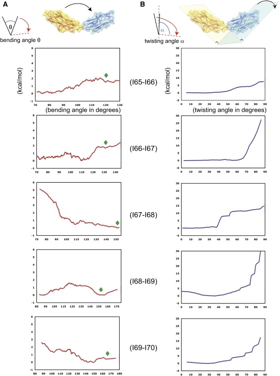
ABF simulations probing the tertiary structure elasticity of titin Ig6. ABF simulations were carried out on each of the connected Ig-domain pairs to probe the energetics of two types of motions: (A) a hinge-bending motion in which the domains bend away from each other at the flexible linker, and (B) a hinge-twisting motion corresponding to a twisting of the chain. In panel A, the potential of mean force (PMF) is shown as a function of the bending angle, with the position observed in respective equilibrium simulations marked by green diamonds. In the panel B, the PMF is plotted as a function of twisting angle, measured also against the equilibrium position. Bending and twisting motions for a domain pair are coupled, such coupling manifests itself in the overall extension of Ig6, and is discussed in the Supporting Material.

The second set of ABF simulations (simAB-t through simEF-t) sampled the tertiary structure elasticity related to the twisting motions between adjacent domains, illustrated in Fig. 4 B. Beginning from the structures of each Ig-pair derived from equilibrium simulations (simEQ-ab through simEQ-ef), one domain was twisted away from the other. Fig. 4 B depicts the potential of mean force as a function of the twisting angle, α, for the five Ig pairs. The twisting motion PMFs reveal that small angular deviations (∼α ≤ 40°) encounter little mechanical resistance as a result of domain-domain interactions. However, continued rotation toward larger twisting angles commands a significant energy cost. In the case of the I67-68 pair (simCD-t), steric crowding appears to come into play at lower degrees of twisting angle (∼37° away from equilibrium) compared with the other Ig pairs, the latter not imposing a large penalty to additional twisting until angles between 50 and 60° are reached. The overall trend of PMFs suggest that there exists heterogeneity along an Ig chain with respect to twisting angles as long as the domains adopt moderate interdomain twisting angles, and that significant elasticity can derive from twisting motion.

Hinge motions in Ig pairs produce an elastic multidomain chain

The free-energy profiles for the hinge-bending motions of the tandem Ig-pairs (Fig. 4 A) permit one to describe the collective elastic behavior of Ig6. In Lee et al. (13), a rudimentary multidomain chain model had been constructed by replicating properties of Z1Z2 hinges into a chain. Here we adopt a similar methodology, described in Methods, with the following modifications:

• 1.The free-energy profile of each domain pair opening is not assumed to be harmonic, i.e., the length distribution of domain pair j, p_j(x_j), is not necessarily Gaussian; and
• 2.The free energy of the bending motions of the domain pairs, and consequently their length distributions, do not necessarily have to be uniform, i.e., each p_j(x_j) is different, to reflect the heterogeneity of linker behavior.

Taking the PMF results from Fig. 4 A (V_j(x_j), where j denotes the five domain pairs AB, BC, CD, DE, and EF), the individual length distributions p_j(x_j) were computed via Eqs. 1 and 2 and plotted in Fig. S1 A. The data were then fitted to a sum of two Gaussians (Eq. 5). As seen in Fig. S1 A, the p_j(x_j) distributions are nonidentical and non-Gaussian. The mean end-to-end distance of the domain pair j, ${\overline{x}}_{\text{j}}={\langle x\rangle }_{V_{\text{j}}}$, and the RMSD of the length distribution, ${\sigma }_{\text{j}}={\left[{\langle {\left(x_{\text{j}}-{\overline{x}}_{\text{j}}\right)}^2\rangle }_{V_{\text{j}}}\right]}^{1/2}$, were computed and are shown also in Fig. S1 A. The free parameters used for these calculations are listed in Table S1.

The five bending angles were then connected to form a hypothetical multidomain chain as depicted in Fig. 2 B, and the overall length distribution of this chain, P(X), was computed via Eq. 4 and plotted in Fig. S1 B (black curve). Although each p_j(x_j) is non-Gaussian (Fig. S1 A), the final P(X) closely resembles a Gaussian distribution, as expected from the central limit theorem (Eq. 6, see Methods), with average $\overline{X}=\sum _{\text{j}=1}^5{\langle x_{\text{j}}\rangle }_{V_{\text{j}}}$, and overall RMSD Σ given by ${\Sigma }^2={\sum }_{\text{j}=1}^5{\mathit{\sigma }}_{\text{j}}^2$.

The Gaussian fit is shown in Fig. S1 B (gray curve). $\overline{X}$ agrees well with $\langle X\rangle =\int dXP\left(X\right)X$ (352.3 Å vs. 358.1 Å), and likewise Σ agrees well with ${\left[\int dX{\left(X-\langle X\rangle \right)}^{2}P\left(X\right)\right]}^{1/2}$ (14.9 Å vs. 16.8 Å). The close agreement is quite remarkable as the central limit theorem holds strictly only in the limit N → ∞. This result implies that repeat proteins behave overall like harmonic elastic springs in the limit of weak force (see Methods). As numerous other elastic proteins are also made of repeat domains, e.g., ankyrin, cadherin, and fibrin (20,22,23,40,41), this result (i.e., that repeat proteins in obeying the central limit theorem act as Brownian springs) is of general importance, although it holds only for small extension.

The relationship between mechanical force and arbitrary chain extension was computed using Eq. 11, which, in terms of the probability distributions p_j(x_j), is

$$\langle X\rangle =\sum _{\text{j}=1}^5\left[{\int }_{-\mathrm{\infty }}^{+\mathrm{\infty }}{x}_{\text{j}}{p}_{\text{j}}\left(x_{\text{j}}\right)\exp \left[f{x}_{\text{j}}/k_{\text{B}}T\right]d{x}_{\text{j}}/{\int }_{-\mathrm{\infty }}^{+\mathrm{\infty }}{p}_{\text{j}}\left(x_{\text{j}}\right)\exp \left[f{x}_{\text{j}}/k_{\text{B}}T\right]d{x}_{\text{j}}\right]\text{.}$$ (18)

The chain extension, i.e., 〈X〉 − 〈X〉_{f = 0}, versus applied force f, is plotted in Fig. S1 C (dashed trace). At low forces (f < 5 pN), the force-extension relation displays the linear behavior (Fig. S1 C, inset) given by Eqs. 12 and 13, derived in the small force limit, with effective spring constant k_c = k_BT/Σ²_soft/stiff, ${\Sigma }_{\text{soft}/\text{stiff}}^2={{\sum }_{\text{j}}{\sigma }_{\text{j}}}^2$, where j includes all five domain pairs, both soft and stiff. One can compute the value of k_c, and obtains k_c ≈ 0.005 k_BT/Ų. When force increases, the chain departs from the linear regime, becoming stiffer, as represented by an increased slope in the force-extension curve, corresponding to opening of the stiffer hinges. At ∼40 Å extension when both soft hinges (BC and DE) are maximally opened (note Δx_{soft, max} = Δx_{BC, max} + Δx_{DE, max} ≈ 40 Å), the slope of the force-extension curve increases to $k_{\text{B}}T/{{\sum }_{\text{j}}{\mathit{\sigma }}_{\text{j}}}^2$, where now j = AB, CD, and EF, i.e., j counts mainly the three stiff hinges. To determine the appropriate f_chain(x), one employs again Eq. 18 to obtain 〈X〉 = g(f). The value g(f) being a monotonic function of f, i.e., ∂g/∂f > 0 as demonstrated in Supporting Material, one can determine (x = 〈X〉) f(x) = g⁻¹(x). f_chain(x) was then plugged into Eq. 17 and the applied force as a function of Ig6 extension during the SMD simulation was computed numerically. The result is plotted as a blue trace in Fig. 3 B.

At most, a ∼70 Å extension $\left(\Delta x_{\text{soft},\text{max}}+\Delta x_{\text{stiff},\text{max}}={\sum }_{\text{j}=1}^5\Delta x_{\text{j},\text{max}}\approx 70\AA \right)$ can be reached through forces of a few tens of pN, i.e., for extensions deriving purely from domain-domain bending (Fig. S1 C). Beyond 70 Å extension, the tertiary structure elasticity due to domain-domain bending is exhausted. To describe the tertiary structure elasticity over a wider range, i.e., over the interval [0 Å, 100 Å], one should account for all other degrees of freedom that permit stretching of up to 100 Å. An obvious choice is domain twisting (neglected so far). In this case, the maximum extension is calculated to be ${\sum }_{\text{j}=1}^{10}{\Delta }_{x\text{j},\text{max}}=93$ Å (see Fig. S1 C, gray trace; details on the calculation presented in Fig. S2 and Table S2). The Ig6 extension under SMD pulling, including both bending and twisting motions in the chain, was calculated again via Eq. 17 and plotted as a red trace in Fig. 3 B. It is noteworthy that f_chain(x) accounting for bending and twisting renders the overall chain softer than it does if only bending is accounted for (Fig. S1 C, inset). Every further degree of freedom accounted for renders a chain overall softer; a stiff degree of freedom adds less “softness” than a soft degree of freedom.

Extension beyond 93 Å involves stretching of individual Ig domains. Significant further extension would lead to rupture of domain secondary structure, but small extension involving reversible (on a nanosecond timescale) domain stretching is permitted without rupturing of secondary structure. To determine the underlying force-extension characteristic of individual domains, we determined U_j(x_j) for single domain extension by simply monitoring x_j(t) for the individual domains as described in the Supporting Material to obtain the RMSD value of x_j(t) for each domain (Fig. S3). The resulting value measured ∼0.6 Å, which corresponds to a force-extension curve for the overall stretching of I65-I70 of $f_0\left(x\right)=\sqrt{k_{\text{B}}T/\left(6\times {\left(0.6\AA \right)}^2\right)}\left(x-x_{\text{eq}}\right)$, where x_eq = 93 Å is the equilibrium length of Ig6 after straightening it through domain-domain bending and twisting. Fig. S1 C shows the force-extension curve for Ig6 determined after the procedure above, adding to domain-domain bending and twisting (black solid curve). As shown by Fig. 3 B (orange trace), inclusion of the stretching degree of freedom reproduces the simulated force response of the Ig6 chain during SMD pulling very clearly. At extension x = 100 Å, this force assumes a value of 200 pN, which is sufficient to rupture the secondary structure of individual Ig domains (i.e., at this extension, the secondary structure elasticity regime of Ig6 sets in).

Secondary structure elasticity of titin I65-70

Force spectroscopy experiments unfolding polyprotein Ig-chains have produced a distinct sawtooth force-extension profile interpreted as the sequential rupture of individual Ig-domains (5–9,42,43). All-atom MD simulations up to this point have been limited by computational resources and by the availability of relevant structures to simulating the unfolding of only single Ig-domains (16,17,19,44). Recent strides in computational efficiency permit us now to carry out SMD simulations to completely extend and unfold titin Ig6.

After equilibrating the Ig6 structure (simEQ-str1), the N-terminal α-carbon of titin I65 was fixed and a stretching force applied to the α-carbon of the C-terminus of titin I70 in simSTR1, employing a constant velocity protocol (28) with v = 25 Å/ns, until all six domains had ruptured and fully extended. The resulting force-extension curve (Fig. 5 A) shows clearly individual force peaks. These peaks, labeled (ii)–(vii), are correlated with the unraveling of individual Ig-domains, producing a sawtoothlike profile similar to those seen in experiment. The drop in force after each force peak, i.e., the domain unraveling event, indicates a relief in stress along the Ig-chain. A detailed view of the structural dynamics reveals that the domain unraveling in every case is initiated by the separation of the terminal β-strands that are adjacent in each domain forming between them 7–9 hydrogen bonds. This strand separation has been described in detail previously (17,20,45). As the internal β-strands, less stable than the terminal β-strands, readily unravel, the β-strands of unruptured domains are permitted to relax and stabilize their interstrand hydrogen bonding. Peak (ii) corresponds to the rupture of I65, (iii) to I70, (iv) to I66, (v) to I67, (vi) to I69, and (vii) to I68. Thus, the order of domain unraveling is I65 → I70 → I66 → I67 → I69 → I68, with the terminal domains rupturing before the ones in the middle of the Ig chain. A schematic of the rupture sequence is provided in Fig. S5 along with a further discussion. Fig. 5 B shows snapshots of the individual domain rupturing events at the timepoints labeled (i)–(vii). The full unfolding trajectory for simSTR1 is available as Movie S2 and Movie S3.

Figure 5.

SMD simulation for full unfolding of titin Ig6. (A) Force-extension curve from sim-STR1, in which the entire I65-70 Ig-domain was stretched until completely unfolded. Instead of simultaneously exhibiting rupturing across all domains, domains unfold one-by-one, producing a sawtooth pattern in the force extension profile. (B) Force peaks in (A) corresponding to ruptures of individual domains are denoted by numerals, corresponding to the close-up views of domain rupture. The domains rupture in the order I65 → I70 → I66 → I67 → I69 → I68.

Additionally, a short simulation (sim-RF) exploring the refolding of Ig-domains was performed, starting from partially unfolded I65 and I70 domains. Although I70 was observed to refold as it had just crossed the terminal β-strand rupture barrier when the force was released for relaxation, I65 (which was more extended at the beginning of the equilibrium simulation) was not observed to refold on the timescale investigated (see Fig. S7 along with further details in the Supporting Material).

Simulation simSTR2 was carried out to stretch Ig6 containing internal disulfide bonds across Cys residues in domains I65, I66, I67, and I69 and to test whether altering the mechanical stability of individual Ig-domains alters the sequence of domain rupture. It turned out that the sequence of rupture remained identical to that observed in simSTR1 without crosslinked cysteines. Details for these simulations are presented in Fig. S6; the trajectory of the simulation is shown in Movie S5 and Movie S6.

Discussion

The titin I-band, which includes the segment Ig65-Ig70, has been experimentally characterized as an exceptionally flexible region of titin, having elastic properties derived from its multidomain architecture of Ig-like, PEVK, N2B, and other disordered domains (1). The elasticity of titin I-band exhibits three complementary extension regimes (13):

• 1.A regime of soft entropic elasticity due to the disordered N2B and PEVK regions;
• 2.A regime of soft, so-called tertiary structure elasticity due to domain-domain bending and twisting as well as minor domain stretching; and
• 3.A stiff, so-called secondary structure elasticity due to the rupture of the β-strand structure of individual Ig-domains.

The latter two regimes have been the focus of this theoretical-computational study, made possible through the availability of the structure of the I65-I70 segment.

Tertiary structure elasticity of titin I-band segment I65-I70

Tertiary structure elasticity is due to bending and twisting motions involving the hinges between neighboring titin domains. The motions change, by Δx, the overall segment length x. Five bending and five twisting degrees of freedom (labeled j = 1, 2, … 10) contribute to an increase of x by Δx_j along with weak stretching of each of the six domains (labeled $j=11,12,\dots ,16$). An overall elastic extension of segment I65-I70, $\Delta x={\sum }_{\text{j}=1}^{16}\Delta x_{\text{j}}$, is assumed to arise in quasiequilibrium with the segment's remaining degrees of freedom and are governed by additive potentials of mean force V_j(x_j). An external force, f, applied adds a potential −f x_j to each contributing degree of freedom and has been shown to lead to the average extension

$$x=\langle X\rangle =\sum _{\text{j}=1}^{16}({\langle x_{\text{j}}\exp \left[f{x}_j/k_{\text{B}}T\right]\rangle }_{V_{\text{j}}}/{\langle \exp \left[f{x}_{\text{j}}/k_{\text{B}}T\right]\rangle }_{V_{\text{j}}})=g\left(f\right)\text{.}$$ (19)

The value g(f) is a fundamental function characterizing the force-extension relationship, f(x) (i.e., the elastic behavior of biopolymers in general), as it can be inverted to yield f(x) = g⁻¹(x). This description has been shown in the molecular dynamics simulations presented above to be highly accurate, to a degree seldom found in the theory of biopolymers. The analysis outlined reveals that titin segment I65-I70 upon application of forces in the range [0, 200 pN] extends up to 100 Å. The analysis, based on g(f), can be applied to any biopolymer system in the reversible stretching regime; the extension function g(f), accordingly, deserves further investigation.

Stiff secondary structure elasticity

Steered molecular dynamics simulations, in many previous studies, captured the force-induced unraveling of individual protein domains. Examples include unraveling of individual fibronectin type-III domains (18,46,47), spectrin repeats (48), fibrinogen coiled-coils (40), and titin domains such as I1 (45,49), and I91 (7,16,17). In the case of this article, the size of the simulations was increased to include stretching and unraveling of six connected Ig domains, allowing direct comparison to experimental results (namely the sawtooth force-extension trace (43)). Specifically, one observes that once a domain ruptures, tension is immediately relieved for all other domains along the chain, illustrating how each Ig-domain functions as a shock absorber for protecting other domains in the chain from forced rupture.

Putting the pieces of the picture together into an elasticity hierarchy

It is now understood that titin's elastic response to forced stretching stems from the mechanical properties of its many constituent domains. The flexibility of these domains contributes to two distinct regimes of elasticity—1), a soft regime characterized by the rearrangement of protein tertiary structure and unraveling of disordered segments during protein elongation, and 2), at physiologically extreme forces, a regime characterized by the rupture of secondary structure folds of individual domains. Computational studies of single titin domains have contributed to this understanding by revealing that it is the network of hydrogen bonds, spanning the terminal β-strands of individual Ig-domains, which governs titin's secondary structure elasticity. The MD simulations on titin I65-70 reported here demonstrate additionally how the domain-domain arrangements and motions give rise to tertiary structure elasticity of titin's flexible I-band. Combining these insights with clues from prior experimental and computational studies, a picture of titin's mechanical properties emerges as a complex molecular spring. Many of nature's other mechanical proteins likely share mechanisms that employ multiple regimes of elasticity for bearing and transforming forces in cells (50).

References

- 1.Tskhovrebova L., Trinick J. Titin: properties and family relationships. Nat. Rev. Mol. Cell Biol. 2003;4:679–689. doi: 10.1038/nrm1198. [DOI] [PubMed] [Google Scholar]
- 2.Labeit S., Kolmerer B. Titins: giant proteins in charge of muscle ultrastructure and elasticity. Science. 1995;270:293–296. doi: 10.1126/science.270.5234.293. [DOI] [PubMed] [Google Scholar]
- 3.Linke W.A., Ivemeyer M., Kolmerer B. Nature of PEVK-titin elasticity in skeletal muscle. Proc. Natl. Acad. Sci. USA. 1998;95:8052–8057. doi: 10.1073/pnas.95.14.8052. [DOI] [PMC free article] [PubMed] [Google Scholar]
- 4.Granzier H.L., Labeit S. The giant protein titin: a major player in myocardial mechanics, signaling, and disease. Circ. Res. 2004;94:284–295. doi: 10.1161/01.RES.0000117769.88862.F8. [DOI] [PubMed] [Google Scholar]
- 5.Rief M., Gautel M., Gaub H.E. Reversible unfolding of individual titin immunoglobulin domains by AFM. Science. 1997;276:1109–1112. doi: 10.1126/science.276.5315.1109. [DOI] [PubMed] [Google Scholar]
- 6.Carrion-Vazquez M., Oberhauser A.F., Fernandez J.M. Mechanical and chemical unfolding of a single protein: a comparison. Proc. Natl. Acad. Sci. USA. 1999;96:3694–3699. doi: 10.1073/pnas.96.7.3694. [DOI] [PMC free article] [PubMed] [Google Scholar]
- 7.Marszalek P.E., Lu H., Fernandez J.M. Mechanical unfolding intermediates in titin modules. Nature. 1999;402:100–103. doi: 10.1038/47083. [DOI] [PubMed] [Google Scholar]
- 8.Li H., Linke W.A., Fernandez J.M. Reverse engineering of the giant muscle protein titin. Nature. 2002;418:998–1002. doi: 10.1038/nature00938. [DOI] [PubMed] [Google Scholar]
- 9.Fowler S.B., Best R.B., Clarke J. Mechanical unfolding of a titin Ig domain: structure of unfolding intermediate revealed by combining AFM, molecular dynamics simulations, NMR and protein engineering. J. Mol. Biol. 2002;322:841–849. doi: 10.1016/s0022-2836(02)00805-7. [DOI] [PubMed] [Google Scholar]
- 10.Watanabe K., Muhle-Goll C., Granzier H. Different molecular mechanics displayed by titin's constitutively and differentially expressed tandem Ig segments. J. Struct. Biol. 2002;137:248–258. doi: 10.1006/jsbi.2002.4458. [DOI] [PubMed] [Google Scholar]
- 11.Oberhauser A.F., Hansma P.K., Fernandez J.M. Stepwise unfolding of titin under force-clamp atomic force microscopy. Proc. Natl. Acad. Sci. USA. 2001;98:468–472. doi: 10.1073/pnas.021321798. [DOI] [PMC free article] [PubMed] [Google Scholar]
- 12.Grützner A., Garcia-Manyes S., Linke W.A. Modulation of titin-based stiffness by disulfide bonding in the cardiac titin N2-B unique sequence. Biophys. J. 2009;97:825–834. doi: 10.1016/j.bpj.2009.05.037. [DOI] [PMC free article] [PubMed] [Google Scholar]
- 13.Lee E.H., Hsin J., Schulten K. Secondary and tertiary structure elasticity of titin Z1Z2 and a titin chain model. Biophys. J. 2007;93:1719–1735. doi: 10.1529/biophysj.107.105528. [DOI] [PMC free article] [PubMed] [Google Scholar]
- 14.Lee E.H., Gao M., Schulten K. Mechanical strength of the titin Z1Z2-telethonin complex. Structure. 2006;14:497–509. doi: 10.1016/j.str.2005.12.005. [DOI] [PubMed] [Google Scholar]
- 15.Linke W., Grutzner A. Pulling single molecules of titin by AFM—recent advances and physiological implications. Eur. J. Phys. 2008;456:101–115. doi: 10.1007/s00424-007-0389-x. [DOI] [PubMed] [Google Scholar]
- 16.Lu H., Isralewitz B., Schulten K. Unfolding of titin immunoglobulin domains by steered molecular dynamics simulation. Biophys. J. 1998;75:662–671. doi: 10.1016/S0006-3495(98)77556-3. [DOI] [PMC free article] [PubMed] [Google Scholar]
- 17.Lu H., Schulten K. The key event in force-induced unfolding of titin's immunoglobulin domains. Biophys. J. 2000;79:51–65. doi: 10.1016/S0006-3495(00)76273-4. [DOI] [PMC free article] [PubMed] [Google Scholar]
- 18.Gao M., Craig D., Schulten K. Structure and functional significance of mechanically unfolded fibronectin type III1 intermediates. Proc. Natl. Acad. Sci. USA. 2003;100:14784–14789. doi: 10.1073/pnas.2334390100. [DOI] [PMC free article] [PubMed] [Google Scholar]
- 19.Best R.B., Fowler S.B., Clarke J. Mechanical unfolding of a titin Ig domain: structure of transition state revealed by combining atomic force microscopy, protein engineering and molecular dynamics simulations. J. Mol. Biol. 2003;330:867–877. doi: 10.1016/s0022-2836(03)00618-1. [DOI] [PubMed] [Google Scholar]
- 20.Lee E.H., Hsin J., Schulten K. Discovery through the computational microscope. Structure. 2009;17:1295–1306. doi: 10.1016/j.str.2009.09.001. [DOI] [PMC free article] [PubMed] [Google Scholar]
- 21.Keten S., Buehler M. Strength limit of entropic elasticity in β-sheet protein domains. Phys. Rev. E Stat. Nonlin. Soft Matter Phys. 2008;78:1–7. doi: 10.1103/PhysRevE.78.061913. [DOI] [PubMed] [Google Scholar]
- 22.Sotomayor M., Corey D.P., Schulten K. In search of the hair-cell gating spring elastic properties of ankyrin and cadherin repeats. Structure. 2005;13:669–682. doi: 10.1016/j.str.2005.03.001. [DOI] [PubMed] [Google Scholar]
- 23.Sotomayor M., Schulten K. The allosteric role of the Ca2+ switch in adhesion and elasticity of C-cadherin. Biophys. J. 2008;94:4621–4633. doi: 10.1529/biophysj.107.125591. [DOI] [PMC free article] [PubMed] [Google Scholar]
- 24.von Castelmur E., Marino M., Mayans O. A regular pattern of Ig super-motifs defines segmental flexibility as the elastic mechanism of the titin chain. Proc. Natl. Acad. Sci. USA. 2008;105:1186–1191. doi: 10.1073/pnas.0707163105. [DOI] [PMC free article] [PubMed] [Google Scholar]
- 25.Darve E., Wilson D., Pohorille A. Calculating free energies using a scaled-force molecular dynamics algorithm. Mol. Simul. 2002;28:113–144. [Google Scholar]
- 26.Rodriguez-Gomez D., Darve E., Pohorille A. Assessing the efficiency of free energy calculation methods. J. Chem. Phys. 2004;120:3563–3578. doi: 10.1063/1.1642607. [DOI] [PubMed] [Google Scholar]
- 27.Hénin J., Chipot C. Overcoming free energy barriers using unconstrained molecular dynamics simulations. J. Chem. Phys. 2004;121:2904–2914. doi: 10.1063/1.1773132. [DOI] [PubMed] [Google Scholar]
- 28.Isralewitz B., Gao M., Schulten K. Steered molecular dynamics and mechanical functions of proteins. Curr. Opin. Struct. Biol. 2001;11:224–230. doi: 10.1016/s0959-440x(00)00194-9. [DOI] [PubMed] [Google Scholar]
- 29.Phillips J.C., Braun R., Schulten K. Scalable molecular dynamics with NAMD. J. Comput. Chem. 2005;26:1781–1802. doi: 10.1002/jcc.20289. [DOI] [PMC free article] [PubMed] [Google Scholar]
- 30.MacKerell A.D., Jr., Bashford D., Karplus M. All-atom empirical potential for molecular modeling and dynamics studies of proteins. J. Phys. Chem. B. 1998;102:3586–3616. doi: 10.1021/jp973084f. [DOI] [PubMed] [Google Scholar]
- 31.MacKerell A.D., Jr., Feig M., Brooks C.L., 3rd Extending the treatment of backbone energetics in protein force fields: limitations of gas-phase quantum mechanics in reproducing protein conformational distributions in molecular dynamics simulations. J. Comput. Chem. 2004;25:1400–1415. doi: 10.1002/jcc.20065. [DOI] [PubMed] [Google Scholar]
- 32.Buck M., Bouguet-Bonnet S., MacKerell A.D., Jr. Importance of the CMAP correction to the CHARMM22 protein force field: dynamics of hen lysozyme. Biophys. J. 2006;90:L36–L38. doi: 10.1529/biophysj.105.078154. [DOI] [PMC free article] [PubMed] [Google Scholar]
- 33.Jorgensen W.L., Chandrasekhar J., Klein M.L. Comparison of simple potential functions for simulating liquid water. J. Chem. Phys. 1983;79:926–935. [Google Scholar]
- 34.Gao M., Sotomayor M., Schulten K. Molecular mechanisms of cellular mechanics. Phys. Chem. Chem. Phys. 2006;8:3692–3706. doi: 10.1039/b606019f. [DOI] [PubMed] [Google Scholar]
- 35.Sotomayor M., Vásquez V., Schulten K. Ion conduction through MscS as determined by electrophysiology and simulation. Biophys. J. 2007;92:886–902. doi: 10.1529/biophysj.106.095232. [DOI] [PMC free article] [PubMed] [Google Scholar]
- 36.Evans E., Ritchie K. Dynamic strength of molecular adhesion bonds. Biophys. J. 1997;72:1541–1555. doi: 10.1016/S0006-3495(97)78802-7. [DOI] [PMC free article] [PubMed] [Google Scholar]
- 37.Izrailev S., Stepaniants S., Schulten K. Molecular dynamics study of unbinding of the avidin-biotin complex. Biophys. J. 1997;72:1568–1581. doi: 10.1016/S0006-3495(97)78804-0. [DOI] [PMC free article] [PubMed] [Google Scholar]
- 38.Sornette D. Springer; Heidelberg, Germany: 2006. Critical Phenomena in Natural Sciences. [Google Scholar]
- 39.Park S., Schulten K. Calculating potentials of mean force from steered molecular dynamics simulations. J. Chem. Phys. 2004;120:5946–5961. doi: 10.1063/1.1651473. [DOI] [PubMed] [Google Scholar]
- 40.Lim B.B., Lee E.H., Schulten K. Molecular basis of fibrin clot elasticity. Structure. 2008;16:449–459. doi: 10.1016/j.str.2007.12.019. [DOI] [PubMed] [Google Scholar]
- 41.Sotomayor M., Schulten K. Single-molecule experiments in vitro and in silico. Science. 2007;316:1144–1148. doi: 10.1126/science.1137591. [DOI] [PubMed] [Google Scholar]
- 42.Williams P.M., Fowler S.B., Clarke J. Hidden complexity in the mechanical properties of titin. Nature. 2003;422:446–449. doi: 10.1038/nature01517. [DOI] [PubMed] [Google Scholar]
- 43.Sarkar A., Caamano S., Fernandez J.M. The mechanical fingerprint of a parallel polyprotein dimer. Biophys. J. 2007;92:36–38. doi: 10.1529/biophysj.106.097741. [DOI] [PMC free article] [PubMed] [Google Scholar]
- 44.Lu H., Schulten K. Steered molecular dynamics simulations of force-induced protein domain unfolding. Proteins: Struct. Funct. Gen. 1999;35:453–463. [PubMed] [Google Scholar]
- 45.Gao M., Lu H., Schulten K. Unfolding of titin domains studied by molecular dynamics simulations. J. Muscle Res. Cell Motil. 2002;23:513–521. doi: 10.1023/a:1023466608163. [DOI] [PubMed] [Google Scholar]
- 46.Craig D., Krammer A., Vogel V. Comparison of the early stages of forced unfolding for fibronectin type III modules. Proc. Natl. Acad. Sci. USA. 2001;98:5590–5595. doi: 10.1073/pnas.101582198. [DOI] [PMC free article] [PubMed] [Google Scholar]
- 47.Craig D., Gao M., Vogel V. Tuning the mechanical stability of fibronectin type III modules through sequence variations. Structure. 2004;12:21–30. doi: 10.1016/j.str.2003.11.024. [DOI] [PubMed] [Google Scholar]
- 48.Altmann S.M., Grünberg R.G., Hörber J.K. Pathways and intermediates in forced unfolding of spectrin repeats. Structure. 2002;10:1085–1096. doi: 10.1016/s0969-2126(02)00808-0. [DOI] [PubMed] [Google Scholar]
- 49.Gao M., Wilmanns M., Schulten K. Steered molecular dynamics studies of titin I1 domain unfolding. Biophys. J. 2002;83:3435–3445. doi: 10.1016/S0006-3495(02)75343-5. [DOI] [PMC free article] [PubMed] [Google Scholar]
- 50.Qin Z., Kreplak L., Buehler M.J. Hierarchical structure controls nanomechanical properties of vimentin intermediate filaments. PLoS One. 2009;4:e7294. doi: 10.1371/journal.pone.0007294. [DOI] [PMC free article] [PubMed] [Google Scholar]
Associated Data
This section collects any data citations, data availability statements, or supplementary materials included in this article.