Abstract
Despite major advances in x-ray sources, detector arrays, gantry mechanical design and especially computer performance, one component of computed tomography (CT) scanners has remained virtually constant for the past 25 years—the reconstruction algorithm. Fundamental advances have been made in the solution of inverse problems, especially tomographic reconstruction, but these works have not been translated into clinical and related practice. The reasons are not obvious and seldom discussed. This review seeks to examine the reasons for this discrepancy and provides recommendations on how it can be resolved. We take the example of field of compressive sensing (CS), summarizing this new area of research from the eyes of practical medical physicists and explaining the disconnection between theoretical and application-oriented research. Using a few issues specific to CT, which engineers have addressed in very specific ways, we try to distill the mathematical problem underlying each of these issues with the hope of demonstrating that there are interesting mathematical problems of general importance that can result from in depth analysis of specific issues. We then sketch some unconventional CT-imaging designs that have the potential to impact on CT applications, if the link between applied mathematicians and engineers/physicists were stronger. Finally, we close with some observations on how the link could be strengthened. There is, we believe, an important opportunity to rapidly improve the performance of CT and related tomographic imaging techniques by addressing these issues.
1. Introduction
Computed tomography (CT) is a global business with several major manufacturers and many minor providers, especially of niche systems. Worldwide sales of CT scanners is more than $2.3 billion per year [1], despite economic slowdown. CT has become the mainstay of modern radiology, often as the first and only examination needed before treatment is administered. Numerous generations of CT hardware have emerged, despite the constancy in the mathematical basis of reconstruction methods. But, why has the pace of innovation in CT reconstruction algorithm front-line applications been so slow? The reasons are not obvious and seldom discussed.
The title of this review poses a question meant to provoke applied mathematicians and image-reconstruction experts to consider closer collaboration with engineers who design tomographic systems and vice versa. Many review articles on x-ray tomographic imaging can be found in the literature [2–6]. Therefore, instead of another review article on the topic, we discuss observations on the translation of research related to x-ray tomography algorithms into clinical and related applications. We realize that some of the comments are admittedly authors’ opinions. It is redundant to exhaustively survey the entire story of x-ray tomography that has been well covered in the extensive literature in the field. We intend our dis cussion to draw the attention of mathematicians to issues concerning the translational research on algorithm development of image reconstruction and its applications in CT.
Technical development in CT has been rapid in recent years. Progress in electronics and detector technology has reached the point where volume scans are performed in seconds, and it is possible to acquire high-quality images of dynamic anatomy such as the heart [7–9]. The pace of hardware development shows no sign of slowing since dual-energy CT is rapidly emerging [10–12], and photon-counting technology with energy resolving capability will make spectral CT a clinical reality in the future [13, 14]. Given all these hardware developments, the algorithms used for image reconstruction in advanced commercial cone-beam scanners remain, however, largely modifications of a filtered-backprojection (FBP) algorithm, which was developed originally for approximate image reconstruction from circular cone-beam data by Feldkamp, Davis and Kress (FDK) about 25 years ago [15–20].
Certainly over the past 25 years, there has been much theoretical progress, especially reported in Inverse Problems, in finding solutions to the x-ray transform, which is the imaging model used in CT. Over the past few decades, the theoretical progress on tomography solutions has been quite astounding. Optimization-based approaches to image reconstruction have yielded efficient forms of iterative algorithms that address physical factors such as noise: there are many forms of the projection onto convex sets (POCS) (or, equivalently, the algebraic reconstruction technique (ART)) [21–23] and expectation-maximization (EM) algorithms [24–26] that converge rapidly and have been demonstrated to work well with real CT data. Also, there has been substantial theoretical progress in developing analytic inverses for the x-ray transform under acquisition conditions under which x-ray projections can be taken by illuminating only a portion of the subject [27, 28].
In many ways, the situation for CT-image-reconstruction-algorithm development is similar to the field of high-temperature (i.e., high-Tc) superconductivity. The first high-temperature superconductors (superconducting above 77 K, the boiling point of liquid Nitrogen) were first developed in 1986, and research in this area has been furious ever since. But as of yet, there is hardly any penetration into industrial application, for example, MRI still uses Helium-cooled superconductors. Perhaps this example also gives us a clue to the lack of proliferation of image-reconstruction-algorithm know-how. Aside from technical difficulties of high-Tc materials, the applications of super-conductivity are limited to quite expensive, niche pieces of equipment, where changing from low-Tc would be an incremental improvement from a business point of view. If on the other hand, the use of superconducting, levitating trains were widespread, the impetus to go to high-Tc would be much greater, spurred by a strong need to reduce cost.
Similarly, as CT scanners are presently designed, the gain in image quality, for everyday-CT applications, in moving away from FBP/FDK-based algorithms is, for the most part, incremental. As such, there appears to be little motivation for a manufacturer to expend resources to implement the latest theory for inverting the x-ray transform, when there are many other practical issues in the development of CT systems: detector arrays, mechanical detector-source rotation speed, pre-reconstruction problems such as correcting for physical factors, including partial-volume averaging, beam polychromaticity, and scatter; and post-reconstruction, display and analysis of 3D/4D image data sets.
Unlike the high-Tc field, we can be much more nimble, because we, in algorithm development, are not bound by physics; it is generally easier for an algorithm specialist to put together an algorithm for a specific purpose such as CT-image reconstruction, than it is for a high-Tc scientist to whip up a new high-Tc superconductor with desirable physical properties. This point leads us to recommend to applied mathematicians who want to see the fruits of their research actually used in a medical scanner to get involved in plug-and-play algorithm development, as described in section 3.
The major issue is communication. The gulf between CT engineers and applied mathematicians is large. It is difficult for engineers to keep up on all advances in applied mathematics. In the optimization community, there is more of an attempt at communication as there are computer codes available for many recent algorithms. But even these can be difficult to adapt to image reconstruction in CT. There are a few of us who specialize in researching image-reconstruction theory and algorithms specifically for CT, but our numbers are too small to effectively bridge this gap. This is clear considering at the attendance of the conference on fully 3D image reconstruction [29] held only every other year, where certainly less than a hundred ‘permanent’ image-reconstruction researchers worldwide, split among all forms of 3D imaging, meet to exchange ideas specifically on tomographic image reconstruction. Thus, the main goal of this review is to give our view on how this gap can be narrowed for more effective, translational research.
The outline of this review goes as follows. Section 2 presents an overview of image-reconstruction design and data flow in a CT scanner. Section 3 specifies what we mean by the development of plug-and-play algorithms. In section 4, we take a look at a particular example of recent theoretical development pertaining to image-reconstruction theory, namely the field of compressive sensing (CS), and give our view on how it may impact on image reconstruction in CT. We use this as an example of how attacking a specific problem may allow deeper penetration of theoretical ideas into practical application. Section 5 sketches the development, using straight-forward theoretical tools, of a few plug-and-play algorithms for image reconstruction that combat confounding issues that come up in CT. These algorithms will belong to the optimization-based class, where due to its history in nuclear medicine imaging, signal noise has been the primary concern in the algorithm development [30]. Noise, however, is unlikely to be such a dominant factor in CT as that in nuclear medicine, despite the great interest in dose reduction in CT. With an eye toward translation, section 6 gives examples of radical changes in CT system/scanning design, where traditional FBP reconstruction cannot be used, and a use of a modern algorithm is necessary. Finally, we point out in section 7 some impediments to translational research from the industrial side and conclude in section 8, with some general recommendations for improving translational research.
2. Chains of algorithm development and data flow in reconstruction
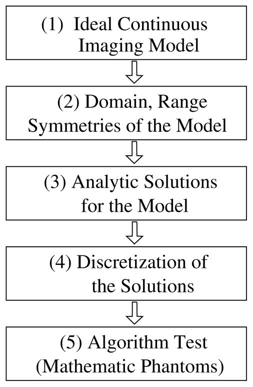
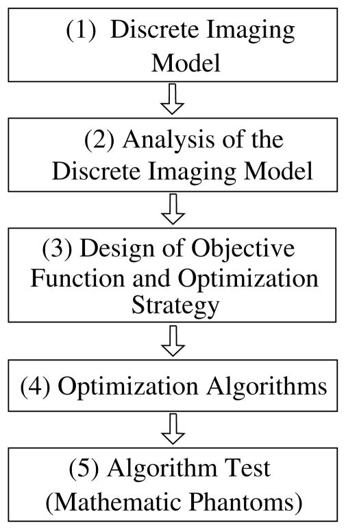
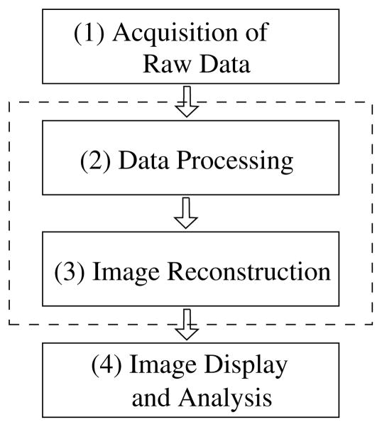
We present three different chains: (1) the chain of algorithm development based on an analytic inverse of the x-ray transform, (2) the same except based on an optimization approach and (3) the chain of data flow in a scanner. While the first chain of analytic algorithm development is considered a standard approach, the second chain is less well developed, and its current mode of operation is essentially borrowed from tomographic image reconstruction in nuclear medicine imaging where iterative image reconstruction has become the norm. Optimization-based algorithm design for CT has definitely some important differences. Furthermore, recent work in CS adds a new dimension to optimization-based-algorithm design. The third chain summarizes the data flow in a CT system. We discuss it to make it clear what the role of image reconstruction is in the scanner. This is important to understand for a couple of reasons: the main one is proper perspective—it makes little sense to spend endless time and effort refining an inversion formula for an idealized imaging model when there are some compromising factors earlier in the data-flow chain, or when the gain in image quality pertaining to the imaging task is incremental, and the other reason is that various factors may be considered either with data pre-processing or taken into account in the imaging model that the reconstruction algorithm inverts.
Algorithm development depends critically upon the imaging model considered. Without loss of generality, we consider in this review only a linear imaging model. However, the observations and insights discussed are likely to be applicable to nonlinear imaging models.
2.1. Chain of analytic algorithm development
The chain of analytical algorithm development can be summarized in figure 1: (1) based upon physics and engineering knowledge of the imaging process and system, an imaging model is devised. In CT, the imaging model is often the x-ray transform of an object function f (r⃗):
| (1) |
where r⃗0(λ) denotes the source location at view λ and θ̂ indicates the direction of the ray. (2) A great deal of research effort from the applied mathematicians has been devoted to the investigation of the properties of the data model, such as its domain, range, symmetries and invertibility. (3) Using knowledge of the properties of the imaging model, one can develop analytic algorithms. It is not uncommon that simplifications have to be made to the model so that an analytic solution can be derived. (4) Discrete forms of the solutions have to be devised because synthetic or real data are always in a discrete form. (5) Algorithms in their discrete forms will be tested largely in mathematical phantom studies. However, because of the various constraints such as the lack of access to real data, little further validations are carried out using experimental data measured in real CT imaging, and this is often the end of the research chain on analytic algorithm development. When real data studies are considered, errors are likely to be introduced in the design of imaging model and algorithm discretization. In fact, a traditional approach in hardware development is to design and build CT systems for yielding data satisfying as much as possible the conditions required by the FBP-based algorithms. As such, the use of the FBP in commercial CT scanners could be attributed, at least partially, to this hardware-development approach.
Figure 1.
Chain of major steps in the development of analytic algorithms.
2.2. Chain of optimization-based algorithm development
The chain of optimization-based algorithm development can be summarized in figure 2: (1) unlike an analytic algorithm that is based generally upon a continuous model, the optimization-based algorithm is based upon a discrete linear equation,
Figure 2.
Chain of major steps in the development of optimization-based algorithms.
| (2) |
where the elements in vectors g⃗ and f⃗ of finite dimensions denote data measurements and image-voxel values, and X indicates the system matrix. (2) Methods such as the singular-value decomposition (SVD) method can, in principle, be used for analyzing the properties of the system matrix X, the methods are unfortunately impractical because of the tremendous matrix size (109 × 109) involved in a typical cone-beam CT problem. (3) Design of the objective function and optimization strategy constitutes a critical step in the chain in which, in addition to the data constraint, prior conditions are also devised and included. (4) Optimization algorithms will need to be selected or developed based upon the properties of the objective function and optimization strategy. (5) The optimization-based algorithms will be tested largely, again, in mathematical phantom studies. For the same reasons mentioned above for analytic algorithm development, little further validations are performed involving experimental data measured in real CT imaging, and this is thus also the end of the chain of the optimization-based algorithm development.
In real-data studies, it is unlikely that the collected data are generated precisely from a discrete image of finite dimension. Also, in simulation studies, in an attempt to mimic the continuous natural of the object function, data can be generated from a continuous object function. Obviously, in these situations, the use of the linear model in equation (2) would introduce inconsistencies in reconstructed images. We will use concrete examples below to illustrate the impact of such inconsistency on reconstructed images. A unique feature of the linear system in equation (2) is that, for given data g⃗, different dimension sizes of the image vector f⃗, and consequently, of matrix X, can be chosen, thus leading to different reconstructions.
It should be emphasized that the developments of analytic and optimization-based algorithms start from distinctive models, i.e., a continuous model in equation (1) and a discrete model of finite dimensions in equation (2). Although the continuous model may be exploited for the design of the discrete model, there is, in general, no direct connection between the two models. However, when the data and object functions in equation (1) are expanded in terms of corresponding discrete basis sets, an approximate discrete linear model may be obtained.
2.3. Chain of data flow in image reconstruction
The chain of data flow is summarized in figure 3: (1) raw data are collected using a CT scanner in real experiments or generated using computer programs in simulation studies. (2) Because raw data are generally contaminated by a number of physical factors that are not included in the imaging model, raw data will undergo corrections to remove the effect of dominant physical factors. (3) Following data correction, images can be reconstructed by use of either analytic algorithms in discrete forms or optimization-based algorithms. (4) The reconstructed images are subsequently displayed and analyzed for applications. In general, on a commercial diagnostic scanner, it is possible to extract raw data in the chain, while the steps of data correction and image reconstruction often form a tightly coupled pipeline that generally allows no intermediate data storage.
Figure 3.
Data flow in CT imaging. With assistance from the vendors of commercial diagnostic scanners, it is possible to extract raw data in the chain, while the steps of data correction and image reconstruction form a tightly coupled pipeline (indicated by the dashed lines) that generally allows no intermediate data storage.
2.4. Algorithm comparison
Image-quality assessment is a huge topic that has been under investigation much longer than x-ray tomography. Strategies and methodologies have been developed for meaningful evaluation of image quality [31–33], and some of them have begun to be applied to evaluating CT images in recent years [34, 35]. It has been well understood in the community of medical imaging research that, depending upon practical imaging tasks, the algorithm performance can vary significantly in terms of the selected evaluation metrics. For example, detection and estimation tasks are two types of tasks encountered often in medical imaging that require very different image properties. Also, it is not uncommon that medical CT images contain some artifacts. However, in many cases, the impact of the artifacts on human-observer performance appears to be minimum. Indeed, the concept that the evaluation of image quality (or algorithm performance) should be task specific has become a general consensus in the field of medical imaging, and methodologies have been developed for task-specific imaging quality evaluation.
It is not our intention to survey the field of image-quality assessment. Instead, we point out that the comparison of algorithm performance in terms of the algorithm’s mathematical exactness may not always be meaningful in practical imaging applications. The ‘mathematical exactness’ of an algorithm is only meaningful when it is with respect to the selected imaging model. However, it is always the case that the imaging model provides only an approximation of a realistic imaging process because it does not consider all of the physical factors occurring in the imaging process. Therefore, even if an exact algorithm can be devised for a selected imaging model, its reconstruction will differ from the underlying object function involved in the imaging process. Furthermore, as the chains in figures 1–3 show, it is likely that a series of approximations such as discretization and interpolations have to be invoked in an algorithm in its application to real, discrete data. Therefore, in the presence of these unavoidable approximations in the design of a practical model and algorithms, any evaluation metrics and studies that are depending only upon the ‘mathematical exactness’ of an algorithm are unlikely to yield meaningful information about the algorithm utility in practical applications.
3. Plug-and-play algorithm development versus traditional theoretical, algorithm research
Most of the research devoted to image reconstruction aims at developing new solutions to solving imaging model problems. The idea being that the imaging model problems evolve toward realistic situations and that this theory eventually finds its way into application. We submit that this style of research is not effective for translation based simply on the empirical evidence that not much of the work published in Inverse Problems over the past couple of decades is actually used in a CT scanner.
Here, we would like to promote another style of research that could have a potentially greater impact on translation of algorithm development to medical and commercial application and may also contribute to theoretical understanding of image reconstruction in CT. We feel, particularly, in x-ray CT that the time is ripe for theoreticians to get involved in the development of plug-and-play algorithms. By plug-and-play development, we mean developing image-reconstruction algorithms, using possibly well-known (among theorists) techniques or theoretical concepts which are not completely, mathematically characterized, that can take actual CT-scanner data and produce useful images, where ‘useful’ can have many meanings depending on the application of the scanner. But generally speaking, what we mean by ‘useful’ is that the algorithm shows advantages on realistic test images or true scanner data. Performance with realistic tests lowers the mathematical bar in the sense that no convergence proofs may be required and that heuristics can guide development. On the other hand, it requires the theorist to think like an engineer or to place themselves in the position of the scanner user, to identify the important factors and to use their bag-of-tricks to cobble together an image-reconstruction algorithm. Such plug-and-play development would greatly facilitate the transfer of knowledge from applied mathematicians to CT engineers, and there will also be reverse flow of knowledge where some important theoretical point emerges in the attempt to adapt image-reconstruction theory to an application. Engineers often have clever ways to overcome various algorithm issues that can be generalized to new ideas for the mathematics of inverse problems or image-reconstruction theory.
Those of us working in the x-ray CT field can consider ourselves lucky in that scanner data can be converted to a form where a fairly simple imaging model, the x-ray transform, is actually an excellent approximation. Thus, on the face of it, it seems that novel inversion techniques for the x-ray transform should slide easily over to the application side. And, over the past decade, there has been extraordinary advancement in x-ray-transform inversion from both the point-of-view of analytic and optimization-based inversions. Yet, not much of this work has contributed to improving commercial CT scanners.
We first explain the issue specifically in relation to work we have been involved with on the analytic inversion of the x-ray transform. In the last several years, analytic algorithms have been developed for exactly recovering an object function from its cone-beam x-ray transforms for a wide class of imaging configurations [28, 36–43]. However, depending upon the practical conditions, the algorithms may not yield images with ‘quality’ superior to those obtained with empirical, approximate algorithms in practical applications. For example, the backprojection-filtration (BPF) algorithm developed recently can yield a mathematically exact reconstruction for helical imaging configuration under ideal, continuous condition [37]. However, in real-world CT imaging, the data collected are far from satisfying the ideal imaging model: a number of physical conditions are necessarily to be considered in the implementation of the algorithm. First of all, the discrete form of the algorithm must be designed because only discrete data are available. More still, it is often the case that data are sampled on non-uniform grids because of the detector-assembling constraint. Therefore, depending upon how the algorithm is implemented (or, equivalently, approximated from its analytic form), its performance in real-world applications is not always guaranteed to be superior to that of some of the optimized, approximate algorithms. In addition to the approximation issues involved in the discrete implementation of theoretically exact algorithms, the ideal data model (i.e., the x-ray transform) upon which the exact algorithms are based provides only approximation to the real data, which contain physical factors such as noise and scatter.
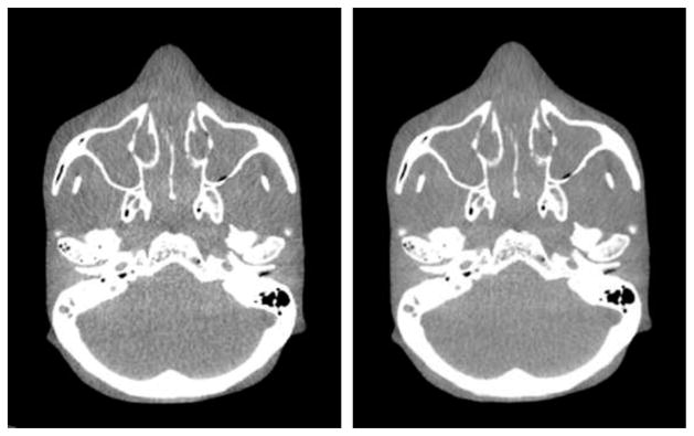
In figure 4, we display images reconstructed using the mathematically exact BPF algorithm and the approximate FDK algorithm from a head-scan data set collected by use of a 64-slice clinical CT scanner with a helical scanning configuration of a pitch = 23.2 mm. For this case, as the results show, although the images appear slightly different, it is unlikely that they will have significantly practical utility difference.
Figure 4.
Reconstructed images from real helical cone-beam data by use of the FDK (left) and BPF (right) algorithms. The display window: [100 HU, 500 HU].
This example suggests that the practical advantages of ‘theoretically exact’ algorithms in real-world applications, if there is any, can be marginal in some cases due to approximations that must be invoked in the design of imaging model and the implementation and application of the ‘theoretically exact’ algorithms. Obviously, research on theoretical issues such as the domain, range, symmetry and invertibility of an imaging model is of interesting and high significance [44–51]. However, it is also important to appreciate the implication of practical issues for the algorithm applicability and flexibility and the fact that the lack of ‘theoretical exactness’ may not be a serious issue in some practical applications. In fact, approximate algorithms can be tailored to, and optimized for, image reconstruction, as demonstrated continuously in established applications. Of course, there may exist opportunities for newly developed ‘theoretically exact’ algorithms to impact significantly on future, new applications in which the approximation-based algorithms are yet developed and optimized.
Both theoretical and practical issues need to be considered in the development of a practically useful algorithm. For example, what we thought was a flexible, theoretically exact algorithm turns out not to be flexible in an important way: detector height fixed but pitch can be variable in practical applications. Another example is that the theoretical investigation of the symmetry of (or, equivalently, the consistency condition on) an imaging model can be an important problem of research because it can provide valuable feedback to the optimization and implementation of algorithms in practical applications. We must point out that researchers are aware of these translational issues. Examples of such effort include the research on full-detector utilization, dose modulation and exploitation of data redundancy for improving algorithms’ numerical properties [52–55].
It is really an issue of division of research effort. The bulk of the applied-mathematics-research effort seems to go toward developing advanced techniques that will likely never be used in practice or address problems that have little application. Two of the authors are guilty of writing such articles. Of course, we feel that improving the theoretical understanding of x-ray-transform inversion is important. But what we hope to convince others of is that: (1) plug-and-play algorithm development is also important, interesting and rewarding; and (2) it is important specifically for applied mathematicians or theoreticians to get involved in designing plug-and-play algorithms in order to bridge a knowledge gap to CT engineers.
As currently, in our opinion, analytic inversion of the x-ray transform is on the tail-end of a huge expansion, and optimization-based inversion is on the verge of an even greater expansion. This review will focus mostly on examples of plug-and-play algorithms considering the optimization-based approach.
4. Compressive sensing and optimization-based algorithms
In light of the above discussion on how to translate theoretical image-reconstruction developments to use in practical applications, we take a specific example of the CS field [56–58]. CS is an excellent example of a field that claims to drive toward practical applications and can potentially contribute greatly to tomographic image reconstruction. As one of the first practical applications of CS to tomography involves sparse Fourier transform inversion, its application to magnetic resonance imaging (MRI) is being heavily pursued [59–61]. From our own experience, many of the ideas in CS are powerful and have helped us to design potentially useful image-reconstruction algorithms for CT. We have adapted constrained, TV-minimization to CT [62, 63] and exploited non-convex optimization [64] to digital breast tomosynthesis [65, 66]. Further work in CT considers practical issues such as including prior scan information [67] and subject motion [68]. CS is also finding its way into other tomographic applications such as diffraction tomography [69] and microwave-based cloud tomography [70].
In addition to image-reconstruction algorithms, CS may offer tools that aid in tomographic system design. Optimization-based image reconstructions often involve very large system matrices that cannot be analyzed by traditional methods such as SVD, and, as a result, system design is based often on intuition acquired from analytic inverses. CS concepts such as the restricted isometry property (RIP) [58], which we discuss in depth below, or related concepts such as incoherence [71], may prove to be useful analysis tools that can be applied directly to the discrete systems of optimization-based image reconstruction.
Although CS has a great potential for CT and some research is being performed to strengthen this link, the gulf between CT scanner engineers, who will implement algorithms for a commercial scanner, and inverse-problem mathematicians is, in our opinion, too large for effective translation. (How many papers in CS deal with Gaussian random matricies versus linear systems modeling real sensors?) We feel that the onus is on the theoretician to explain the theory at a level where it is widely understandable, making sure not to overstate advantages and to clearly explain limitations, and to step back from complete generality to look at application to particular systems. For CS, we attempt, here, to explain what it means for image reconstruction in CT. In no way do we wish to claim that presentation is complete and methods described are optimal. The following should just be regarded as a temporary, pontoon bridge linking CS to CT that will hopefully be replaced by future, more solid work.
4.1. CS and CT
CS theory aims at providing exact signal recovery from noiseless, but undersampled measurements. Furthermore, signal recovery appears to be robust in many undersampled cases; namely, low levels of noise in the data lead to small inaccuracies in the recovered signal. An important CS concept for signal recovery for a linear system such as that in equation (2) is the RIP [58]. The isometry constant of X is the smallest number δs such that
| (3) |
holds for all s-sparse vectors f⃗, where s-sparse means that f⃗ has at most s non-zero entries. Based on the RIP, the solution of equation (2) may be possible for ill-conditioned or under-determined X. If δs = 1, there are s-sparse vectors in the null space of X, and recovery of an s-sparse signal is impossible. For designing CS-based signal-recovery algorithms for s-sparse vectors, it is important to consider the isometry constant δ2s. If δ2s is sufficiently less than 1, then any pair of s-sparse signals will have a degree of distinguishability in the data space. Based on certain ranges of the isometry constants δs and δ2s, various CS algorithms can be shown to arrive at exactly the underlying s-sparse signal f⃗ even when the size of g⃗ is much smaller than would be necessary for direct inversion of equation (2). The RIP analysis is potentially useful for CT-system design; one could imagine designing a system with fixed numbers of measurements such that δ2s is minimized, where s is the expected sparsity of a typical signal.
The problem with the RIP analysis, however, is that it is only a sufficient condition, and it has been used only for proving recovery for a quite restricted set of matrices that involve forms of random sampling [58]. For system matrices modeling CT, or most other linear imaging models, the RIP analysis is on the face of it quite limited [72]. A major problem is that the isometry constants change upon transformation by an invertible matrix G. Transforming equation (2),
| (4) |
leads to a linear system with the same solution space, but the isometry constants derived from
| (5) |
can be quite different than those derived from equation (3). It is true that altering the multiplication by G may alter performance of algorithms solving the linear system, but the change in isometry constants does not seem to reflect only pre-conditioning by G. For example, if G is diagonal with equal diagonal elements, G represents simple scaling, which should have no pre-conditioning effect. On the other hand, such a scaling can dramatically modify isometry constants. Despite this fact, the RIP concept can still potentially be useful in a practical sense for specific applications as pointed out in section 4.1.3.
In any case, we present a small simulation that is quite suggestive that CS methods may be useful for image reconstruction in CT. Consider the following optimization:
| (6) |
where
| (7) |
The ℓ0-norm is counting the number of non-zero image pixels. Accordingly, the optimization problem in equation (6) finds the sparsest f⃗ that agrees with the available data g⃗.
We illustrate CT-image reconstruction from projection data generated from the gradient magnitude of the discrete Shepp–Logan phantom, shown in figure 5. We consider image reconstruction of a 128 × 128 image from projection data containing 25 views and 256 bins on the detector. Just from vector sizes, this reconstruction problem is under-determined: there are about 16 K pixels and 6.4 K transmission measurements. For CT, even equal number of samples and image variables often lead to an ill-posed system matrix, due to ill-conditioning. Therefore, this particular configuration represents a substantial reduction in the number of views by roughly a factor of 10.
Figure 5.
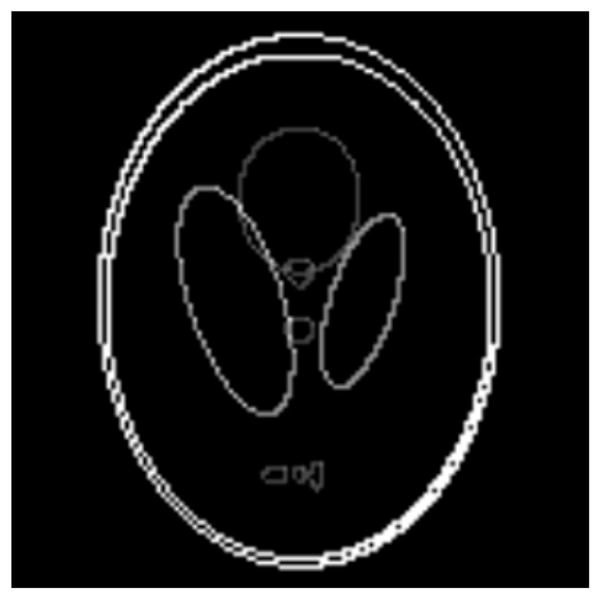
Gradient magnitude of the discrete Shepp–Logan phantom on a 128 × 128 grid.
4.1.1. CS-image reconstruction
In order to perform the image reconstruction, we use a CS-based algorithm: iterative, hard-thresholding (IHT) [73], which finds a solution to an optimization problem related to equation (6):
| (8) |
This problem constrains the image to have sparsity s, and among these images, finds the one that agrees with the data. In the simulation study, data g⃗ is generated from a phantom with sparsity s = 1085. Accordingly, we run IHT with this sparsity and observe if image recovery is possible. (In actual application the signal sparsity is unknown, but the algorithm can be run for various values of s and the smallest s yielding a small data error can be a criterion for sparsity selection.)
We select IHT mainly because of its simplicity and ability to handle very large systems, but we expect that the conclusions drawn from this example extend to other CS-based algorithms when applied to CT-image reconstruction. We point out that there can be a restriction on selecting CS-based algorithms because of the very large size of X, which can be of 109 × 109 for cone-beam CT. A pseudo-code IHT can be written as follows:
| 1: | μ = 2.0; Niter = 1000 |
| 2: | f⃗ = 0 |
| 3: | for i:= 1, Niter do |
| 4: | f⃗:= Hs (f⃗ + μXT (g⃗ − Xf⃗)) |
| 5: | end for |
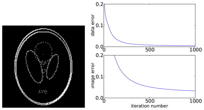
The symbol:= means ‘set the variable on the left to the quantity evaluated on the right’. The operator Hs (·) represents hard thresholding of the argument, where the largest s components are kept and all others are set to zero. The argument of Hs on line 4 is an image update based on gradient descent of the ℓ2 data residual. The value of μ = 2.0 was chosen for fast convergence on this particular example. The study results in figure 6 show that after 1000 iterations IHT nearly comes up with the underlying image even though we are operating the algorithm outside of its proven range.
Figure 6.
Left: reconstructed image by IHT. Right: data error ||g⃗ − g⃗*||ℓ2/||g⃗*||ℓ2 and image error ||f⃗ − f⃗*||ℓ2/||f⃗*||ℓ2 as a function of iteration number, where f⃗* is the discrete phantom and g⃗* = Xf⃗*.
4.1.2. Evolving IHT toward a plug-and-play algorithm for CT
In the image-reconstruction community, it has been known for some time that iterative image reconstruction can often be accelerated by processing blocks of data sequentially or even, in the extreme case, processing each single measurement sequentially. For example, the EM algorithm is often used in tomography but it is known to converge quite slowly. There has been much work aimed at accelerating EM by processing ordered subsets of the projection data [74]. Such ordered subset-EM (OSEM) algorithms generally reduce the number of iterations by a factor close to the number of ordered subsets.
Another popular algorithm that updates the image sequentially with each measurement is the ART, which is also known as the POCS; the convex sets for the ART are the hyperplanes defined by each measurement gi. We can take advantage of the POCS algorithm to improve the efficiency of IHT for image-reconstruction problems. We replace the gradient descent step with a loop that performs one cycle of sequential projections through all measurement rays, obtaining the following IHT-POCS algorithm:
| 1: | Niter = 1000 |
| 2: | f⃗ = 0 |
| 3: | for i:= 1, Niter do |
| 4: | for j:= 1, Nd do: |
| 5: | f⃗:= Hs (f⃗) |
| 6: | end for |
The number of measurements is Nd, and X⃗j is a row of the system matrix corresponding to the measurement gj.
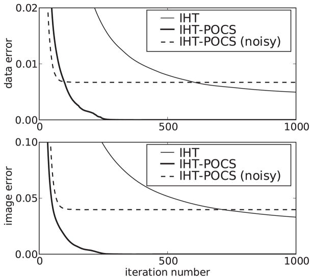
The results for IHT-POCS shown in figures 7 and 8 indicate that there may be some advantage for CS-based algorithms to use sequential or row-action data processing when applied to tomography. Aside from our own CT algorithm, adaptive-steepest-descent (ASD)-POCS [62, 63], we know of only one other work that proposes a row-action algorithm for CS application [75].
Figure 7.
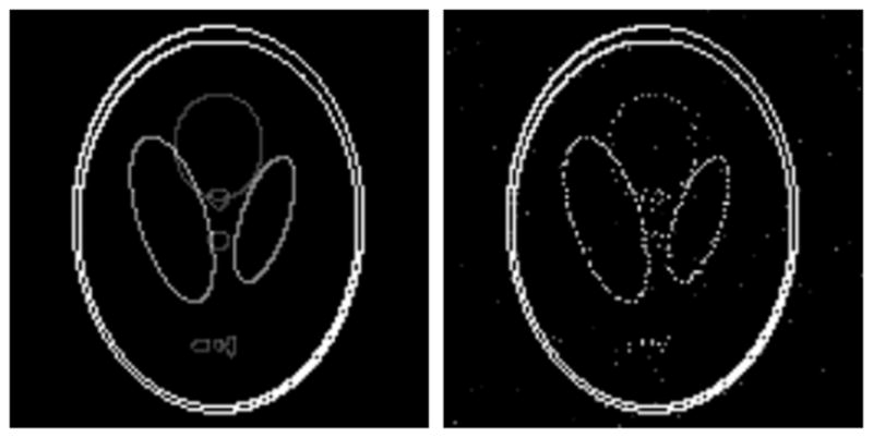
Reconstructed image by IHT-POCS from (left) noiseless data and (right) noisy data with multiplicative Gaussian noise.
Figure 8.
Errors as a function of iteration number for IHT and IHT-POCS. The data error is ||g⃗ − g⃗*||ℓ2/||g⃗*||ℓ2 and the image error is ||f⃗ − f⃗*||ℓ2/||f⃗*||ℓ2, where f⃗* is the discrete phantom and g⃗* = Xf⃗*.
The noisy reconstruction in figure 7 indicates that IHT-POCS may be stable. (We have tested this algorithm with multiple starting images that are sparse, and we have found that the stability of IHT-POCS can be improved by using soft thresholding at line 5, where smaller vector components are reduced by a factor less than 1.0, e.g. multiplying by 0.9, instead of being set to 0, although the number of iterations will likely increase.) Although, as will be seen below, there are many forms of data inconsistency, which may have very different effects on image-reconstruction algorithms. An important point about algorithm efficiency is illustrated in figure 8. Note that the convergence of IHT-POCS to the noisy solution is faster than in the noiseless case. We have found empirically that trying to achieve convergence under ideal, noiseless conditions for CS-based optimization problems can be a trap. Convergence is slow, and once any kind of data inconsistency is considered, convergence improves substantially. The message is that developing the algorithm that is efficient for the ideal case appears to be quite hard, and the effort is likely wasted when it comes to actual applications where there will always be data inconsistency.
4.1.3. What about the RIP?
The accurate and robust reconstruction obtained in this example suggests that there is an underlying theory for accurate image recovery of sparse images in CT from limited data sets. We re-examine the RIP to see if we can use it for developing a tool to analyze the system matrix X. Such tools are lacking for analyzing optimization-based image reconstruction, because X is usually too large for standard analysis such as SVD. The isometry constants can be obtained by looking at the distributions of the quantity:
| (9) |
where we consider G to represent only a scaling. To arrive at the isometry constant δs, σs for all possible s-sparse images needs to be computed. The maximum and minimum values of σs yield δs after the appropriate scaling. While it has been noted that this in general is not practical, some headway can be made when considering specifically the CT application.
Because the set of s-sparse images contains s′-sparse images if s > s′, δs will be larger than δs′. It can be a useful comparison for system matrices corresponding to different configurations to look only at δ1 and δ2, as will be seen in section 6.3. Also, to estimate δs for larger s it is possible to use the fact that the projection sensing matrix X will have the greatest difficulty in distinguishing neighboring pixels. This fact greatly reduces the search space for computing δs.
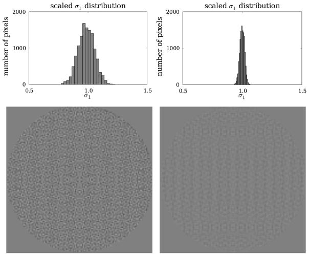
Take, for example, the reconstruction performed above. It was stated that using 256-bin detectors improves recovery of the Shepp–Logan edge phantom over using 128-bin detectors. The scaled distributions of σ1 in figure 9 indicate that δ1 is 0.2283 and 0.0660 for the 128- and 256-bin detectors, and it is clear that the σ1 distribution is narrower for the 256-bin detector. This figure also shows the σ1-map in the field of view of the CT system, where the 256-bin detector yields greater uniformity.
Figure 9.
Top row: histograms of σ1 values, scaled so that resulting δ1 is minimized, for a 2D parallel-beam-CT configuration consisting of 25 views with a 128-bin (left) and a 256-bin (right) detector, and reconstructing onto a 128 × 128 pixel array. Bottom row: the σ1 distributions are created by computing Xf⃗ for all images that contain one non-zero pixel. The images shown for the 128-bin (left) and 256-bin (right) detectors are created by placing the value of σ1 at the location of the non-zero pixel of the corresponding 1-sparse image. The gray scale for the images [0.5, 1.5] and pixels outside of the field-of-view are set to 1.0.
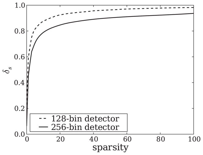
Using the specific structure of the matrix X, we have constructed a program that estimates δs from δs−1 and the corresponding images from which δs−1 is derived. The results for the two configurations are shown in figure 10. While our program is accurate for s = 1 and s = 2, we cannot make any such claims for larger s except that it serves as a lower bound on δs for s > 2. Still, this knowledge may be useful as a guide for system design. We point out that there seems to be an interesting theoretical puzzle, here, because the isometry constants obtained are well above typical bounds used in convergence proofs, yet we have successfully tested the 25-view, 256-bin detector configuration with multiple images with the same sparsity as the Shepp–Logan edge phantom.
Figure 10.
Estimates of δs for sparsities, s ≤ 100. Values are accurate for s ≤ 2 and represent a lower bound for larger s. The lower δs for the 256-bin detector is an indication that this configuration may lead to better image recovery than the configuration with a 128-bin detector.
With this specific example on the RIP, we are trying to get across two points. First, the above analysis is not very deep in a mathematical sense, but it may prove useful to system design and the communication of mathematic concepts from the research front to engineers as long as limitations are expressed. Analysis such as what is discussed here will hopefully be quickly replaced by deeper and more general analysis, but until then it is better than nothing. Second, in the spirit of developing plug-and-play theoretical tools it may be interesting to restrict generality and consider in detail specific systems that are widely used in actual applications.
4.2. Does CS beat the Nyquist frequency?
The claim often made in CS papers is that CS theory can go beyond Nyquist sampling, obtaining exact image reconstruction from fewer samples than are required by Nyquist frequency. This claim reflects the fact that theorems proved for various CS applications reveal conditions for possible ‘exact’ recovery of the underlying signal. This claim, however, is misleading, because CS and Nyquist sampling work under two different assumptions. Nyquist sampling has to do with exact recovery of a continuous signal that is band-limited. CS has to do with exact recovery of a signal that can be represented by a finite set of expansion functions. It turns out that for physical applications such as CT, being able to represent the underlying object function with a truly finite expansion set is quite limiting (this is demonstrated explicitly with an idealized example using the Shepp–Logan phantom in section 5.1.4). On top of this issue, exact recovery is only proved for a quite limited set of linear measurement matrices.
A concrete explanation of this issue is illustrated with CT simulation in section 5.1, using noiseless data generated from the continuous Shepp–Logan phantom. This phantom is piecewise constant, and thus its gradient is highly sparse in a point representation. But it is not possible to recover this image exactly with current CS-based algorithms, because CS does not cover continuous objects and discretization of the image into pixels introduces approximation. As a result, the CS theory applies only approximately to this physical measurement systems. Once CS-based algorithms are used for systems in the domain of approximate applicability, they should be compared with other optimization-based approaches that have been developed for the same system. We point out that what is now called compressive sensing has been a research goal in the image-reconstruction community for some time, and there has been work deriving similar algorithms for limited-angle scanning [76] and few-view angiography [77] that pre-date CS.
While the comparison of the necessary samples for CS and Nyquist serves as a good way to communicate the new results of CS in the original articles, follow-up articles seem to repeat this statement in such a way that there is an implicit superiority of CS to other optimization-based approaches, because CS is implied to be the first theory to break the Nyquist barrier. As a result, newly published CS-based algorithms are often not compared with state-of-the-art, optimization-based algorithms and are instead compared with analytic algorithms where missing data are zero-filled—a highly unrealistic assumption.
Furthermore, thinking in terms of exact recovery can also be quite limiting. Much CS literature is published on sampling with Gaussian random sensing matrices, and not much addresses physical sensing systems such as that in CT.
Likewise, a great deal of the CS effort is now going into algorithm efficiency in solving idealized problems. For applications there are two important points to consider: (1) again, rarely is the exact or numerically exact image needed, and (2) there is always some inconsistency in the data, and convergence properties of algorithms on ideal data might not be terribly meaningful. To echo the second point, in our own research on CS-based algorithms, we have found that our algorithms often take quite long to come up with an accurate solution to optimization problems modeling ideal CT systems compared to those modeling systems with some form of inconsistency (as discussed above). When iterative algorithms are used in practice, they are often severely truncated in terms of iteration number. It is not uncommon for iteration numbers to be truncated at 10 or fewer. One might consider questions such as ‘After N-iterations, how close is the image yielded by algorithm A to the underlying image?’ or ‘After N-iterations, does algorithm A yield a better image than algorithm B?’
Nevertheless, the CS ideas are powerful and will likely aid in designing many useful optimization problems for image reconstruction. We feel that the major impact of CS in tomography will be to focus on algorithm development for high-quality, under-sampled data where efficient algorithms need to be developed that can solve optimization problems with an extremely small number of regularity parameters. Such an example will be presented in the following section.
5. Illustrations of specific issues in CT-image reconstruction
In the previous sections, the discussion on image-reconstruction algorithms has been quite general, but now we illustrate a number of specific issues that come up in trying to develop plug-and-play algorithms. We offer possible solutions with well-known theoretical techniques or algorithms. We focus on issues that tend to be glossed over, because they may be regarded as too specific for any kind of general analysis, and because theoreticians may not appreciate their impact having not actually developed a system from hardware up. On the other hand, for engineers developing systems, they may not be aware that further software advances may ease the burden on system-hardware development.
5.1. Continuous object projection
Cutting edge research on optimization-based image reconstruction considers many important issues such as how to deal with metal in the subject, incorporating realistic noise models, estimating x-ray scatter along with the attenuation map or considering various forms of data incompleteness. These are all important efforts, but when actually considering an optimization-based algorithm for image reconstruction for a commercial scanner, there is a much more basic issue that discourages the shift away from FBP-based algorithms. Even under conditions of ideal, noiseless, pure x-ray transform data, optimization-based algorithms may yield images with conspicuous artifacts.
One large difference between analytic and optimization-based algorithms for image reconstruction is that the image-expansion set plays a large role in the algorithms. It is clear that different image-expansion sets will yield different system matrices in equation (2). The success of the algorithm will depend on how accurately the underlying object function can be represented by the image-expansion set. For a concrete example, we examine image reconstruction from projections of the Shepp–Logan phantom, and we will investigate optimization-based image reconstruction using the standard pixel representation of the image.
The simulated data set consists of 256 views and the detector has 512 bins. With this set of data, a 256 × 256 image representation would avoid an underdetermined linear system. The problem with utilizing 256 × 256 pixels to represent the image, however, is that it does not provide a very good expansion set for the underlying object that is composed of ellipses. The impact of the image pixelization is seen in performing image reconstruction based on minimizing:
| (10) |
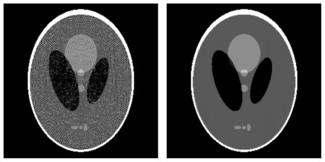
This optimization problem can be accurately solved with the conjugate gradient (CG) algorithm. The resulting image is displayed in figure 11. The artifacts are rather overwhelming, and the data residual is high, at 1.96, because the pixel representation forces the reconstructed image to be constant over the pixel. Note that for this set of imaging parameters, this form of data inconsistency can be much larger than that generated by noise.
Figure 11.
Left: reconstructed image from noiseless projections of the continuous Shepp–Logan phantom. Right: reconstructed image from noiseless projections of the discrete, pixelized Shepp–Logan phantom. Both reconstructions are obtained from the conjugate gradients algorithm for minimizing the quadratic data-fidelity term in equation (10). The gray scale is [0.95, 1.15].
5.1.1. Possible solutions
Most of the solutions to this issue involve changing the expansion set from pixels to other sets that may represent the object function more accurately. For example, pixels (or voxels) have been replaced by blobs or other expansion sets (see [78] and section 4 of [2]). The limitation of such approaches is that alternate expansion sets will improve the image quality only for certain classes of object functions. Changes in the expansion set, in general, will only alter the quality of the artifacts. And presently users of CT are used to some of the streak artifacts in FBP-based reconstructions, and there is not really a huge motivation of exchanging FBP streaks for some other type of artifact.
Another interesting, practical approach is to use different discrete approximations to the continuous projection and back-projection operations. For example, the EM algorithm is often implemented with a ray-driven forward-projection and a pixel-driven back-projection. This strategy essentially introduces a small amount of smoothing at each forward-projection and back-projection operation. Though effective, this approach strays from the optimization-based approach, because it is not clear what optimization problem the algorithm is solving. Alternate discrete projectors have been proposed, such as distance-driven [79], that may improve numerical properties while maintaining that the discrete back-projection is the transpose of the discrete forward-projection.
What is often done is to introduce regularization explicitly. The regularization can be effectively implemented in two ways: (1) explicitly add a roughness penalty term to the data-fidelity objective, and/or (2) truncate a slowly converging algorithm. A simple example of the former is to introduce a quadratic regularity penalty:
| (11) |
where
| (12) |
and
| (13) |
(Indices i and j denote components of the image vector f⃗ specifically for a 2D image, here). The advantage of such an approach is that it can be solved accurately with an algorithm such as CG; the disadvantage is that parameter γ is added to the list of parameters specifying image representation and projection model all of which can greatly affect image quality. Moreover, regularization introduced explicitly here or implicitly with the mis-matched forward-projector/back-projector pair causes a loss of information that might not be necessary. Parameter explosion is one of the challenges that face optimization-based algorithms for image reconstruction in commercial products.
5.1.2. Increased image-expansion set for plug-and-play optimization-based algorithms
Another approach, investigated in [80], which may be more fruitful, is simply to use more elements in the expansion set. It is clear, for example, that using smaller pixels will allow for a better representation of the underlying image. Another important advantage in doing this is that the form of the expansion elements becomes less critical; the difference between using blobs or pixels is smaller when there are more of them. This helps reduce the number of parameters to play with. The mathematical problem in increasing the expansion-set size is that the number of expansion elements may be considerably greater than the number of measurements, so that the linear imaging equation system becomes under-determined. But, here, one of the lessons of CS can be applied. It is fine to have an under-determined system of equations as long as there are some other constraints to help select a ‘good’ image out of the possibly large nullspace of an imaging equation. CS offers the possibility for constraining the system based on image sparseness, but there are other possibilities too.
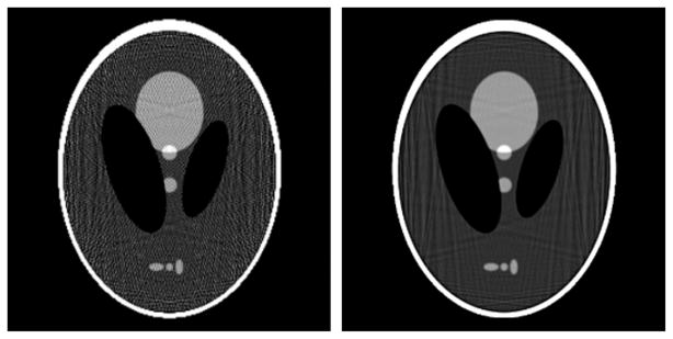
Figure 12 shows the problem of simply increasing the number of pixels. Both images are obtained by solving equation (10) with a zeroed initial estimate. Going to the under-determined system by increasing to 512 × 512 pixels, image quality appears to degrade. Although the image on the right is clearly poorer, its corresponding data error is actually less than that of the image on the left. For under-determined systems a low data error does not correlate always with a low image error, because some other information needs to be fed into the image reconstruction to obtain an accurate estimate of the underlying image.
Figure 12.
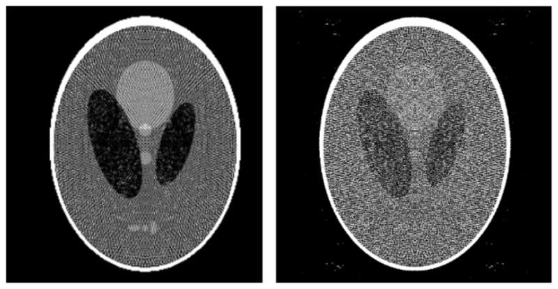
Reconstructed image from noiseless projections of the continuous Shepp–Logan phantom onto a (left) 256 × 256 pixel and (right) 512 × 512 pixel image. Both reconstructions are obtained from the CG algorithm for minimizing the quadratic data-fidelity term in equation (10) with a zero-filled starting image. The gray scale is [0.95, 1.15].
5.1.3. Constrained, quadratic optimization
An example of how to select an image out of the nullspace could be to choose the one with minimum quadratic roughness. A possible formulation for this optimization problem is
| (14) |
where the constraint limits possible images to the ones that agree with the data to within tolerance ε. The minimization of the objective selects the feasible image with smallest roughness. This problem can be shown to be equivalent to equation (11), where smaller values of ε correspond to smaller γ. The case, in which ε = 0 and the constraint becomes g⃗ = Xf⃗, is obtained in the unconstrained optimization by the limit γ → 0.
Using CG to solve the unconstrained problem with γ = 0.005 and an image array of 512 × 512, the image shown in figure 13 is obtained. This image is clearly superior to the 512 × 512 image in figure 12. Also, in going to more pixels the resulting image agrees with the data more closely than for the 256 × 256 case, as the data error for the 256 × 256 case is 2.14 and the 512 × 512 case is 2.05.
Figure 13.
Reconstructed image from noiseless projections of the continuous Shepp–Logan phantom onto a (left) 256 × 256 pixel and (right) 512 × 512 pixel image. Both reconstructions are obtained by use of the CG algorithm for minimizing the quadratic data-fidelity term in equation (11) where γ = 0.001 on the left and γ = 0.005 on the right. The gray scale is [1.0, 1.1].
5.1.4. Constrained TV-minimization—a CS approach
Solving the optimization problem proposed in the CS community also provides a satisfactory algorithm for this image-reconstruction problem. We employ the ASD-POCS algorithm [63] to solve the constrained minimization:
| (15) |
where
| (16) |
and Δi,j is as given in equation (13). The results displayed in figure 14 show clearly that the 512 × 512 image quality is superior to that of the 256 × 256 image, and once again the data error is lower for the image with more expansion elements. The ASD-POCS algorithm permits the inclusion of the positivity constraint without much additional effort.
Figure 14.
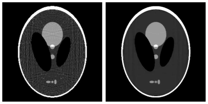
Reconstructed image from noiseless projections of the continuous Shepp–Logan phantom onto a (left) 256 × 256 pixel and (right) 512 × 512 pixel image. Both reconstructions are obtained by constrained, TV-minimization using the ASD-POCS algorithm. The values used for ε are 2.10 on the left and 1.05 on the right. The gray scale is [1.0, 1.1].
With this specific example in hand, a few comments about CS approaches are in order. This particular example should favor a CS approach because the Shepp–Logan phantom is sparse after applying a spatial gradient operator. In comparing figures 13 and 14, the CS image may be only slightly better than the image obtained with a quadratic optimization problem that does not rely on any form of image sparsity (a rigorous comparison would require some quantitative image-quality metrics and a study of a range of optimization parameters). This demonstration is aimed at the CS claim of being able to beat the Nyquist frequency. The present results could be interpreted as some kind of up-sampling, defeating Nyquist sampling, but this would be true of the quadratic optimization method also. Basically, within an optimization framework the quality of the images will depend on how good the assumed prior information is. Thus, we would like to stress again that it is important to compare CS-based algorithms to other optimization-based algorithms and not only to analytic algorithms.
Another related point, with respect to CS beating the Nyquist frequency, is that strictly speaking CS cannot obtain the exact image even in this highly idealized, numerical experiment. The reason being that even though the Shepp–Logan phantom is piecewise constant, its gradient magnitude cannot be represented exactly by the number of pixels smaller than the number of measurements. For the above experiment there are 256 × 512 measurements, and this number of measurements will stay the same no matter how many pixels there are in the image. Embedding the Shepp–Logan phantom into a 256 × 256 pixel image, the resulting gradient-magnitude image has 2184 non-zero pixels. But this embedding entails an approximation. Going to a 512 × 512 image array yields a better approximation to the continuous Shepp–Logan phantom, but the number of non-zero pixels in the gradient-magnitude image has roughly doubled to 4386. It is clear that the Shepp–Logan phantom is represented exactly only in the limit that the pixel size goes to zero, and when the image size passes 16 K × 16 K the number of non-zero pixels in the gradient-magnitude image will exceed the number of measurements, thus any hope of exact recovery is lost. It is, of course, possible that there may be some other representation in which the image can truly be represented sparsely, but it is very difficult to find such expansion sets for other than contrived examples.
Returning to the problem of reconstructing images from a continuous imaging model, the highly accurate reconstructions obtained by both the CG and ASD-POCS algorithms show that going to an over-complete image-expansion set may prove to be a general strategy for optimization-based algorithms. There are likely other effective algorithms based on, for example, the EM algorithm where the data-fidelity constraint is written in terms of the Kullback–Leibler divergence [24]. As a practical point in designing the iterative algorithms for under-determined linear systems, modification of standard algorithms such as CG can improve efficiency. These types of optimization problems involve extremely small regularization parameters or tight constraints, in the constrained version. They are generally more efficiently solved by allowing the regularization parameter to change during the iteration. The CG algorithm employed above starts out with γ = 1.0, and this parameter is decreased during the iteration to its final value. The ASD-POCS algorithm also involves an evolution of constraint tightness. And many other CS-based algorithms use a similar strategy.
5.2. FBP streaks
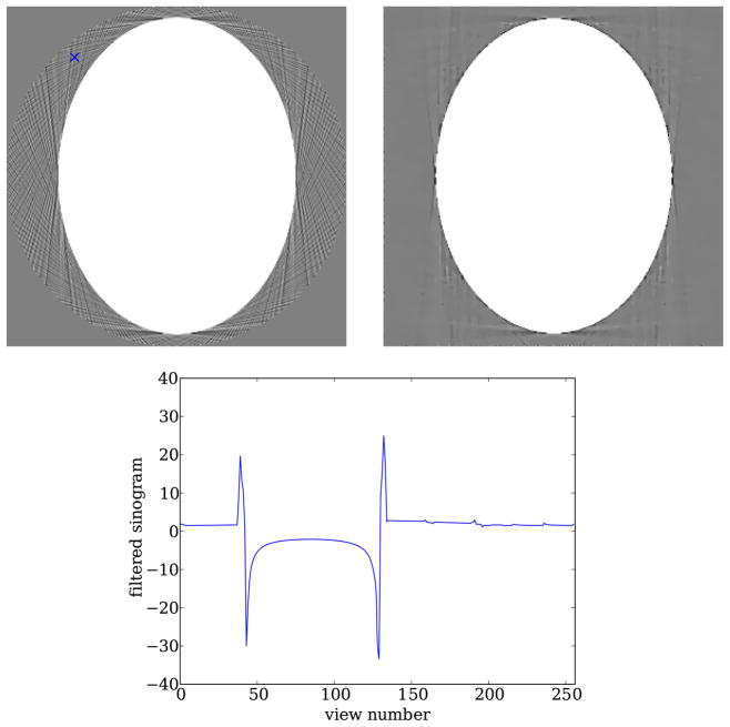
A well-known artifact of analytic algorithms are streaks that occur outside of any region with a discontinuous boundary. The origin of the streaks has been known for some time and is explained for example in [81]. The problem is essentially an angular sampling issue, and it is easily seen in the context of parallel-beam CT as shown in figure 15. From a theoretical point of view, this is a well-understood phenomenon, and there has been some effort to investigate alternative interpolation methods to reduce the impact of data under-sampling. From the industrial point of view, data under-sampling artifacts have motivated the development of expensive hardware solutions such as the development of x-ray sources with a flying focal spot [82]. Thus, there is some practical importance for re-examining this issue to search for theoretical solutions that mitigate artifacts due to data under-sampling, and any algorithm that intends to depose FBP-based algorithms has to address this.
Figure 15.
Left: FBP reconstruction shown in a [−0.05, 0.05] gray scale window. Note the point indicated by the cross, when examining plot on the bottom. Right: same as the 512 × 512 TV-minimization image shown in figure 14 except gray scale window is changed to [−0.05, 0.05]. Bottom: plot of filtered sinogram values that contribute to the point indicated by the cross above. The strong, rapid variations occur for views where the cross lines up with a tangent of the skull. For a continuous sinogram, the ramp-filtered version diverges at such discontinuities. As a result, data discretization has a large impact near these singularities.
Optimization-based image reconstruction may be able to outperform FBP-based image reconstruction in this regard. Using the algorithms from the previous section that employ a large expansion set may be able to reduce the impact of these streaks. Comparing these above reconstruction for a 512 × 512 pixel representation with parallel-beam FBP results in figure 15, it is clear that an optimization-based approach can address the streak-artifact issue. The streaks may possibly be further diminished by going to an even larger image array, or smaller pixel size. Granted, the streaks in the figure are not critical because they are outside of the object support, but one can expect to encounter other subjects with plenty of strong, internal discontinuities. The reduction of streak artifacts by optimization-based algorithms is promising, but there are certainly other factors to consider in the data-flow chain of CT.
5.3. Incompletely corrected data: ‘slow drift’ contamination
As discussed in section 2, in commercial scanners a variety of physical factors are corrected for prior to the application of the image-reconstruction algorithm. Correction for factors such as beam-hardening and scatter, or incident x-ray flux determination is likely to have some level of error. As some of these factors do not have high spatial frequency, there will always be some level of slowly varying background in each projection remaining after the data preprocessing. We demonstrate the potential impact of such a background with the following idealized numerical experiment. Again, we simulated parallel-beam CT projection data of the Shepp–Logan phantom. But we introduce data inconsistencies by adding a random constant offset to each projection, a simplistic model of incomplete physical factor compensation. A plug-and-play image-reconstruction algorithm should consider this type of data inconsistency.
With such a data model, it is clear that FBP-based reconstruction will be unaffected—another reason for the hardiness of FBP. Taking the derivative of the projection data, a component of the ramp filter, effectively kills the constant offset. Another way to see this is that the ramp filter is zero at zero frequency, so the constant background will be filtered out. As a result, the FBP image is highly accurate as seen in figure 16. Optimization-based algorithms, on the other hand, show significant artifacts when the data-fidelity term measures the distance between actual and estimated projection data sets.
Figure 16.
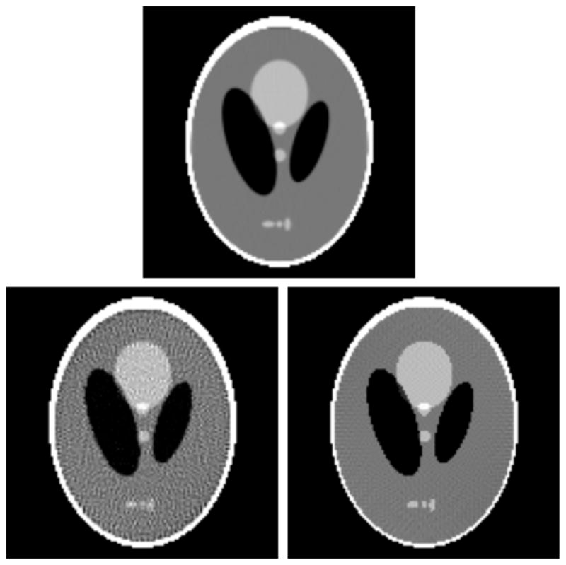
Top row: the FBP image from simulation data generated with the continuous Shepp–Logan phantom for 128 views over 180° and a 256-bin detector. A random constant is added to each view following a Gaussian distribution with standard deviation of 10% of the maximum projection value. Bottom row: images reconstructed from the same data set except that the projections are generated from the discrete Shepp–Logan phantom by optimization using the standard ℓ2 data-norm (left) and an ℓ2 norm on the data derivative (right). These 128 × 128 images solve, respectively, equations (11) and (17) where γ = 0.01. Note that the FBP image is unaffected by the view-random, constant background, that the image reconstructed using equation (11) contains significant artifacts and that the image reconstructed using equation (17) also shows fewer artifacts.
There are two remedies for the optimization-based approach. First, the optimization problem can be altered so that the derivative of the data and estimated data are compared. For example, equation (11) can be altered to
| (17) |
where Du is the discrete operator that performs finite differencing of the projections along the detector. Second, the data can be projected into the range of the x-ray transform. Here, for parallel-beam CT, this involves enforcing that the integration of the projections on the detector yields the same value, and any conjugate rays are made equal. Other moment conditions can also be enforced. The difficulty with enforcing uniform projection integration is that the ‘true’ value of this integral is unknown. In any case, image reconstruction based upon the optimization approach in equation (17) is shown in figure 16.
For plug-and-play algorithm development, it is clearly important to test algorithms against a wide variety of data inconsistencies that can come up in CT, and the above list is certainly not complete. Many articles on image reconstruction, if they consider inconsistent data at all, consider mainly detector noise. Again, we do not want to leave the impression that such detailed studies are not being done, it is really a matter of balance. It is perhaps safe to say that the majority of articles on image-reconstruction algorithms address some theoretical point claiming often to have solved that point. But rarely is a follow-up paper seen where these algorithms are rigorously tested against a host of issues that arise along the CT-data-flow chain. Probably, the feeling is that this is work should be left to a CT engineer, but the fact is that there are far too many ideas out there that are too inaccessible for engineers to systematically search and explore the applied mathematic literature. And often such algorithms get tripped up on some simple practical issues like those mentioned above. Thus, for more effective knowledge transfer, in our opinion, it is up to the reconstruction-algorithm theorists and applied mathematicians to address some of the above issues by developing plug-and-play algorithms.
6. Scanner design motivated by recent developments in image reconstruction
The real progress in moving past FBP-based reconstruction will occur when engineers have real experience with advanced image-reconstruction algorithms and can use this knowledge to design more efficient and effective CT scanners. This development will likely occur first in dedicated CT systems such as head/neck CT, dental CT and breast CT. But it may be possible that, down the road, radical changes in diagnostic CT will occur, enabled by advances in image-reconstruction theory. Based on recent developments in image-reconstruction theory, we sketch a couple of radically different data-acquisition configurations in CT that may have a large impact on delivered dose while maintaining or improving image quality.
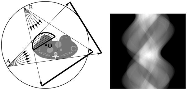
To illustrate these ideas, we stick to 2D fan-beam CT, but each of these ideas generalizes easily to 3D CT. To describe the various acquisitions, it is useful to have a general picture in terms of the 2D full-data space, represented as a 2D rectangle with the horizontal and vertical axes representing the detector-bin and view-angle coordinates, respectively. We show in the right panel of figure 17 a full projection data in a 2D-data space for a fan-beam scanning configuration depicted in the left panel of figure 17 in which non-truncated fan-beam data of the cross-section of a torso phantom are collected over a full angular range of 2π. A number of existing algorithms can readily be used for reconstructing images from the full data set.
Figure 17.
Left: a cross section of a torso phantom is scanned by use of a fan-beam configuration in which the fan beam completely covers the cross section at each of the views over a full angular range of 2π. Right: projection data in the 2D-data space (i.e., the 2D rectangle) with the horizontal and vertical axes representing the detector-bin and view-angle coordinates, respectively.
In figure 18, we display several partitions of the data space each of which corresponds to a scanning configuration of potential practical significance. The partition in the left panel of row 1 corresponds to a half-detector scan, and an image can be reconstructed by use of existing analytic algorithms such as FBP-based algorithms. As illustrated below, the partition in the middle panel of row 1 depicts a minimum data scan in which a region-of-interest (ROI) can be reconstructed exactly by use of analytic algorithms such as the BPF algorithm. Along side with these two partitions, the other partitions shown in figure 18 correspond to a number of theoretical challenges to image-reconstruction theory such as the image-reconstruction problems from data acquired in few-view (right, row 1), limited-angular-range (left, row 2), interior-problem (middle, row 2), and exterior-problem (right, row 2) and in scans with metal objects (left, row 3), bad-detector bin (middle, row 3), and/or an angular-dependent coded aperture (right, row 3). This type of diagram presents a unified picture illustrating various CT-scan designs some of which are discussed below.
Figure 18.
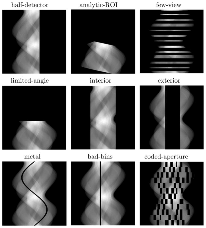
Data-space partitions corresponding to various scan configurations or common CT issues in which knowledge of data function within some portions of the data space is missing. The 2D rectangle represents the data space with the horizontal and vertical axes representing the detector-bin and view-angle coordinates, respectively. Row 1: partitions corresponding to a half-detector scan (left), a scan as illustrated in figure 19 (middle), and a few-view scan (right). Row 2: partitions corresponding to a scan over a limited angular range (left), an interior-problem scan (middle) and an exterior-problem scan (right). Row 3: a scan of the cross section with a metal object (left), a scan with bad detector bin (middle) and a scan with an angular-dependent coded aperture (right).
6.1. Targeted region-of-interest imaging
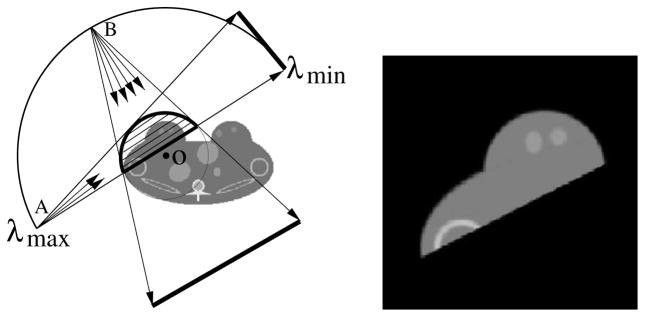
In contrast to the FBP-based algorithms that cannot reconstruct theoretically exactly images from data containing transverse truncations, the BPF algorithm is capable of yielding theoretically exact images within ROIs from data containing certain transverse truncations [27]. As an example, we consider the reconstruction of a region enclosed by the thick curve, as shown in the left panel of figure 19, from fan-beam data. It can be shown that the BPF algorithm requires data collected over an angular scanning range between λmin and λmax as long as the ROI is always covered by the fan-beam illumination at these scanning views. Therefore, the fan-beam illumination can be restricted to cover only the ROI. The fan-beam illumination at two scanning views A and B displayed in the left panel of figure 19 leads to transversely truncated projection data. However, the data do contain data information sufficient for exact image reconstruction within the ROI. The data set sufficient for reconstructing the ROI image in the right panel of figure 19 is displayed in the middle panel of row 1 in figure 18.
Figure 19.
Left: the region enclosed by the thick curve indicates the ROI for imaging, the thin curve between λmin and λmax indicates the source trajectory, and fan-beam rays from source points A and B denote two projections covering only the ROI. The BPF algorithm requires data collected over the angular range over an angular scanning range between λmin and λmax as long as the ROI is always covered by the fan-beam illumination at these scanning views. Clearly, the collected data contain transverse truncations. Right: ROI image reconstructed by use of the BPF algorithm from data containing transverse truncations.
6.2. Few-view CT
In order to obtain an accurate estimate of the continuous data function for the application of analytic algorithms, many views, typically hundreds or more are taken. Clearly, an algorithm that can perform accurate image reconstruction from few views would be of interest in order to realize CT systems that can reduce patient dose and possibly speed up scans. Theoretical research on this problem has been addressed by optimization-based algorithms over the past decade with renewed interest coming recently especially due to CS. The data sampling for the few-view scan is illustrated in figure 18. As demonstrated in [63], in section 4.1 and in figure 21, there are certainly algorithms that can provide accurate image reconstruction for this type of scan. In the left panel of figure 21, we show an image reconstructed from data acquired at 25 views uniformly distributed over 180°.
Figure 21.
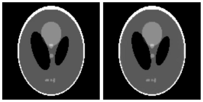
Images reconstructed for few-view CT data (left) and coded-aperture CT data (right). The simulated data are generated from a discrete Shepp–Logan image. The few-view data simulate an acquisition of 25 views over 180°. For the coded-aperture data 128 views over 180° are used and each projection is masked resulting in the data partitioning shown in figure 20.
At first glance, it seems that algorithms capable of few-view image reconstruction should have been incorporated into CT-scanner design, but the issue is more complicated than simply reducing views. The problem can more generally be looked at in a way where the total dose to the patient is fixed. This dose can be divided into a few, high-quality projections or many, noisy projections. Variations on this theme are also possible by considering uneven dose distributions. For few-view CT system to actually be engineered, it is insufficient to demonstrate only that a given algorithm ‘works’ for few-view data. The view-number/dose-per-projection trade-off needs to be carefully studied along with other sources of data inconsistency, some of which were mentioned in section 5.
6.3. Coded aperture for CT
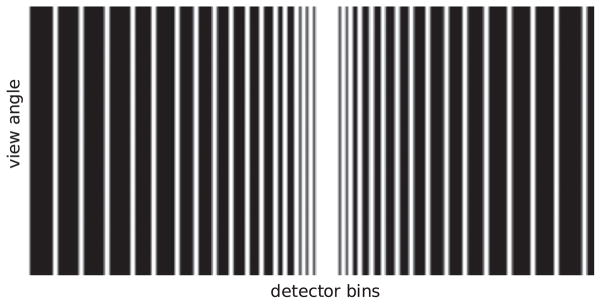
Another radical design, suggested to us by Igor Carron, the keeper of the CS-blog [83], is to send the x-ray source through a coded aperture [84] prior to irradiating the subject, similar to the idea of using a beam-stop array [85] without the additional scan (see the data partition in the right of row 1 in figure 18 for a general, angular-dependent coded-aperture scan). Certainly, from an FBP point of view such a scan makes little sense. But from a CS perspective, it is viable. For an angular-independent-coded-aperture example of which is sketched in figure 20, we reconstructed an image that is displayed in the right panel of figure 21.
Figure 20.
Data partition used for angular-independent-coded-aperture CT. The white regions indicate the sampled part of the data space.
The images shown in figure 21 for both few-view and coded-aperture scanning CT provide evidence that both configurations may serve as the basis for a novel CT design. It may be possible to employ some form of RIP analysis, as discussed in section 4.1 to optimize source locations for a few-view scan or to help design specific forms of the coded-aperture.
The coded-aperture configuration is likely to have a similar dose as the few-view configuration, but in considering the overall CT design there may be an advantage of employing a coded-aperture. As CT systems are evolving toward using large area detectors, the problem of x-ray scatter becomes worse. One of the standard hardware methods of reducing the impact of scatter is to put an anti-scatter grid in front of the detector. Though effective, this grid throws away a fraction of the diagnostic radiation. With the coded-aperture, the radiation is masked prior to entering the patient; thus, the x-ray dose is fully utilized. And x-ray scatter can be accurately estimated and subtracted by measuring x-ray intensities in the shadow of the aperture.
7. Additional impediments to changes in CT algorithms
Among the main reasons for slow progress on introduction of algorithmic innovations into clinical CT scanners may also be the proprietary nature of CT technologies and the subjective evaluation of performance by its users. CT manufacturers must have access to a broad portfolio of intellectual property (IP), some of which is not their own. For example, numerous CT patents may be enforceable and may render it impossible to build a commercially viable unit without infringement on IP held by competing interests. If all of the IP were rigidly separated, we would not have the panoply of high performance helical scanners that are on the market today. Therefore, there is a mechanism where manufacturers can cross-license or share IP and reconcile or allocate the costs without violating anti-monopolistic trade laws and triggering enforcement actions.
Second, much of the essential IP needed to make scanners is not disclosed in the literature or in patents. Each manufacturer has trade secrets that permit them to economically manufacture large numbers of scanners with exceptionally high performance and reliability. Much of this is achieved at a price, since numerous corrections are done to the raw detector measurements before they are entered into the FBP reconstructor. These correction schemes are highly proprietary.
The corrections of the raw detector measurements are based, in large part, on calibration tables constructed for each scanner that are tailored to each individual instrument’s idiosyncrasies and imperfections. For example, when an x-ray tube is exchanged in the field, the manufacturers’ service representatives spend many hours with the replacement, operating the scanner and rebuilding the calibration tables. To meet the acceptance specifications for each scanner, this process is the most important step in image-quality assurance.
Because FBP-based algorithms can be implemented in parallel to achieve clinically useful reconstruction speeds (e.g., up to 100 512 × 512 axial images per second) with off-the-shelf commodity computer hardware and communications components, and since the image quality is acceptable to the community of radiologists and other CT buyers/users, there has been little motivation to change. Engineering teams who are building new scanners have limited time and budgets and avoid technical risk when possible. It is safer to employ the expedient well-known and well-understood FBP than to attempt introduction of, e.g., an iterative alternative. In general, a clinical CT scanner will implement only one reconstruction method (e.g., FBP), with a variety of data conditioning and filtering choices that the operator may select.
Finally, the users and buyers of CT equipment are very familiar with the limitations of FBP-based algorithms (e.g., sensitivity to noise, motion and especially metal), so workarounds are available. There is a general unquestioning acceptance of the status quo in image quality for CT, where the most important parameters recently have been speed, coverage and dose. Faster scanners, with all other factors held constant, have been sufficient to open new application areas such as coronary CT angiography to widespread use. An order of magnitude increase in CT-data-acquisition speed resulted in a greatly expanded market with many new installations as the transition from 16-slice to 64-, 128- and 256- or 320-detector-row scanners has been introduced.
The door to innovation in CT algorithms requires an efficient and practical route to develop and test new algorithms. It is unlikely that any investigator, mathematician or engineer could effectively correct for the raw detector measurements from the CT scanner into a form suitable for algorithm testing without the manufacturer’s blessing and assistance. However, manufacturers of CT scanners, in general, have not made the raw projection data available to anyone outside their organizations, even to customers that use their CT scanners. There are exceptions to this, but not many when compared to the almost universal availability of CT scanners in hospitals and clinics.
There is no Digital Image COMmunication (DICOM) standard for CT raw data [86, 87]. In fact, there are no standards at all. Corrected raw projection-data sets are almost impossible to find in the public domain. Without this data, clinically realistic examples of images cannot be reconstructed. As a consequence, CT-algorithm developers almost universally use highly idealized numerical phantoms for their work and seldom show results obtained with ‘real’ experimental or clinical data. This is surely a major impediment to progress.
On behalf of the manufacturers, generating and exporting corrected raw projection-data sets is not easy. These data sets are verbose, and the corrections are applied on-the-fly during the image synthesis. They are not generally stored and commonly exist only transiently during their transfer and entry into the FBP processing. As a result, we may maintain the raw detector measurements on-line during and after CT scanning, so subsequent processing and multiple reconstructions may be done from the same measurements using the data-correction/FBP pipeline. As an example, for temporal bone CT studies, we may want to change the magnification (voxel size) and center of interest to produce very detailed right and left sided data sets from a single acquisition. A survey set of whole head axial images is reconstructed at low resolution, and with a smaller field-of-view and higher resolution, both right and left side temporal bone data sets are generated—all from a single set of detector measurements. This is universally available in clinical CT scanners today. But the corrected raw CT projections are not. What a pity!
From a practical standpoint, the speed of image reconstruction is very important in clinical applications. Today, it is common for a 64-channel multidetector-row CT scanner to produce 1000 or more axial 512 × 512 reconstructed slices per case, and this may be repeated every 15 min for 10–12 h per day. The pace of image reconstruction from projections, fully corrected for detector and scanner imperfections, may approach 50–100 slices per second using commodity PC hardware or graphical processor unit (GPU), Field Programmable Gate Arrays (FPGA), and Cell hardware [88, 89]. Much of the engineering effort required to produce a state-of-the-art clinical CT scanner is devoted to optimizing the image-reconstruction chain. Data-transfer rates from the gantry to redundant-array-of-inexpensive-disk (RAID), correction and filtration preprocessing, and backprojection produce computational demands that challenge the designers to extract every aspect of performance available. Since the image-reconstruction process is so fundamental to CT, repeated so often, and it is one of the most important sets of operations that influence scanner performance and image quality, there is great reluctance to depart from the very well-known and well-understood FBP/FDK-based reconstruction.
It is important to recognize that clinical CT scanners are very heavily used for a wide variety of applications—angiography, head imaging, abdominopelvic applications, pediatrics, chest and heart. Each application and the variety of patient types—young and old, inpatient and outpatient, and emaciated and obese—all present unique challenges, but the same scanner must be able to do them all. Each scanner typically has one data-acquisition and image-reconstruction pipeline to produce results. It would be possible, e.g., where suppression of metal artifacts or low dose, low noise scanning is required, to implement more than one reconstruction algorithm on a scanner. If the system was ‘open’ and could be refined by algorithm developers in the field, such algorithms could be tested and clinically validated. The benefits of new technology, especially in image-reconstruction algorithms, could reach patients without waiting for their possible inclusion in future generations of CT scanners (because this has not happened for the past 25 years and may not in the near future).
There is a direct correlation between computational performance, power consumption and the number of CT detectors, following the principles that govern semiconductor progress given in Moore’s Law [90]. Of these related technologies, the semiconductor industry, in general, gives long-term projections of their products which can be used to estimate what type of specifications may be realized in imaging instruments for the next 15 years. Presently, the state-of-the-art microprocessors are fabricated at 45 nm and by next year (2010), the successor 32 nm units should be available in quantity. These commodity microprocessors are the basis of CT reconstruction for most clinical scanners, and each successive generation provides the gain in performance predicted decades ago by Gordon Moore [90]. By using low-cost disks and microprocessors, as the number of CT-scanner detectors has grown, the reconstruction processors have kept pace while the underlying FBP/FDK-based algorithms have remained relatively constant. It is feasible to map the anticipated computation performance and link it to requirements of advanced, optimization-based reconstruction algorithms for the foreseeable future using this paradigm.
8. Recommendations for more complete translational research
Briefly, the recommendations to applied mathematicians are (1) to write articles, and especially introductions to articles, that introduce theoretical concepts in an intuitive way that explains how the results may be used in a practical scenario, (2) to develop plug-and-play algorithms for a particular system using existing theoretical know-how and (3) to include a comparison of new methods with existing techniques such as FBK/FDK-based and optimization-based algorithms using ‘real’ data. This means of reporting results can have significant educational value, especially for students. Providing a real-world motivation for algorithm development can stimulate fundamental and enduring progress in applied mathematics by developing a practical algorithm specific to a given system.
On the engineering side, there will be more motivation, and less cost, with greater attention to theoretical developments if articles communicate better, computational performance and image quality with ‘real’ data are provided, and example programs are readily available. Once engineers are aware of the latest theory, the intrinsic benefits and trade-offs relative to FBP/FDK-based algorithms, and have example codes to work from, these mathematical developments can be incorporated into a novel scanner design, thereby leading to imaging devices that enable specific imaging applications. Currently, x-ray imaging is undergoing a renaissance, but movement away from FBP may be desirable, when there is new growth in the variety of tomographic x-ray devices.
The success of applied mathematics in medical imaging should be measured by acceptance of new methods by users and their influence on decision making in research and ultimately for clinical practice. The coupling of mathematical innovation in CT reconstruction methods with clinical imaging has been informal and beset with obstacles. Rapid progress in tailoring algorithms to current and emerging problems in clinical applications could be made by addressing some of the impediments.
Borrowing from success in open-source biomedical visualization (e.g., the visualization toolkit (VTK)) [91–93] and image processing (e.g., the imaging toolkit (ITK)) [94, 95] are possible solutions. These open-source systems provide access to implementation of algorithms, which have been tested and validated using data and software tools that are accessible to anyone who is interested. Although some websites have appeared with CT-reconstruction implementations, a community-based open-source repository and coordinated set of methods with a representative spectrum of corrected raw detector measurements from ‘real’ CT scanners has not. Perhaps the need for an open-source-community-developed CT-reconstruction toolkit (CTK) with a database of corrected raw projection data from real CT scanners will be recognized.
Compressive sensing has attracted broad interest and numerous contributions have been made which are tracked and disseminated in a blog (for web-log) known as Nuit Blanche [94]. This innovative and user-friendly portal is particularly useful, because it not only collects references within CS, but the owner provides excerpts from interviews of CS experts and also maintains there a ‘living document’ called ‘Compressive Sensing: The Big Picture’ which allows non-experts to quickly understand the CS issues and concepts. Such a blog serves as a model that can guide the development of new blogs devoted to a broad spectrum of CT reconstruction topics.
But ultimately, the translation of new mathematical methods for CT reconstruction will not achieve its potential until and unless the developers can access corrected raw detector measurements. The sophistication of major CT users to recognize this issue and require such access as a condition of sale for new instruments will require some action and guidance by the applied mathematics community to alert their colleagues to the potential benefits. It was not trivial to accomplish the standardization of data formats used for medical image interchange, now known as DICOM [86, 87]. The DICOM organization is managed by the National Electronics Manufacturers Association (NEMA) and is a participatory open forum for emerging standards. Among the various DICOM working groups, there is opportunity to develop and disseminate standards for interchange of corrected raw CT data. Industry and medical imaging users are active in the DICOM working groups, but representation by the applied mathematics community is minimal.
The imperatives for CT today and opportunities for growth in applications include lower dose, multi-energy, whole organ (e.g., brain, heart, others) perfusion, and many others. The progress in data acquisition is measured in orders of magnitude over the past two decades, while the image-reconstruction algorithms have not kept pace. Given the central role of CT in current medical practice, algorithmic improvements could achieve broad acceptance, provided that they can be tested and optimized on ‘real’ systems.
Acknowledgments
This work was supported in part by National Institutes of Health (NIH) R01 grants CA120540 and EB000225. EYS was also supported in part by a Career Development Award from NIH SPORE grant CA125183-03. The contents of this review are solely responsibility of the authors and do not necessarily represent the official views of the NIH.
References
- 1.http://www.businesswire.com/news/home/20071030006295/en
- 2.Defrise M, Gullberg G. Image reconstruction. Phys Med Biol. 2006;51:R139–54. doi: 10.1088/0031-9155/51/13/R09. [DOI] [PubMed] [Google Scholar]
- 3.Kalender WA. X-ray computed tomography. Phys Med Biol. 2006;51:R29–43. doi: 10.1088/0031-9155/51/13/R03. [DOI] [PubMed] [Google Scholar]
- 4.Pan X, Siewerdsen J, La Riviere PJ, Kalender WA. Anninversary paper: development of x-ray computed tomography: the role of Medical Physics and AAPM from the 1970s to present. Med Phys. 2008;35:3728–39. doi: 10.1118/1.2952653. [DOI] [PMC free article] [PubMed] [Google Scholar]
- 5.Orth RC, Wallace MJ, Kuo MD. C-arm cone-beam CT: general principles and technical considerations for use in interventional radiology—for the Technology Assessment Committee of the Society of Interventional Radiology. J Vasc Interv Radiol. 2008;19:814–21. doi: 10.1016/j.jvir.2008.02.002. [DOI] [PubMed] [Google Scholar]
- 6.Dobbins JT, Godfrey DJ. Digital x-ray tomosynthesis: current state of the art and clinical potential. Phys Med Biol. 2003;48:R65–106. doi: 10.1088/0031-9155/48/19/r01. [DOI] [PubMed] [Google Scholar]
- 7.Nikolaou K, Flohr T, Knez A, Rist C, Wintersperger B, Johnson T, Reiser MF, Becker CR. Advances in cardiac CT imaging: 64-slice scanner. Int J Cardiovasc Imag. 2004;20:535–40. doi: 10.1007/s10554-004-7015-1. [DOI] [PubMed] [Google Scholar]
- 8.Choi SI, George RT, Schuleri KH, Chun EJ, Lima JAC, Lardo AC. Recent developments in wide detector cardiac computed tomography. Int J Cardiovasc Imag. 2009;25:23–9. doi: 10.1007/s10554-009-9443-4. [DOI] [PubMed] [Google Scholar]
- 9.Walker MJ, Olszewski ME, Desai MY, Halliburton SS, Flamm SD. New radiation dose saving technologies for 256-slice cardiac computed tomography angiography. Int J Cardiovasc Imag. 2009;25:189–99. [Google Scholar]
- 10.Carmi R, Naveh G, Altman A. Material separation with dual-layer CT. IEEE NSS-MIC Conf. Record; 2005. pp. 1876–78. [Google Scholar]
- 11.Flohr TG, et al. First performance evaluation of a dual-source CT (DSCT) system. Eur Radiol. 2006;16:256–68. doi: 10.1007/s00330-005-2919-2. [DOI] [PubMed] [Google Scholar]
- 12.Zou Y, Silver MD. Analysis of fast kV-switching in dual energy CT using a pre-reconstruction decomposition technique. Proc SPIE. 2008:6913–691313. [Google Scholar]
- 13.Shikhaliev PM, Xu T, Molloi S. Photon counting computed tomography: concept and initial results. Med Phys. 2005;32:427–36. doi: 10.1118/1.1854779. [DOI] [PubMed] [Google Scholar]
- 14.Schlomka JP, et al. Experimental feasibility of multi-energy photon-counting K-edge imaging in pre-clinical computed tomography. Phys Med Biol. 2008;53:4031–47. doi: 10.1088/0031-9155/53/15/002. [DOI] [PubMed] [Google Scholar]
- 15.Feldkamp LA, Davis LC, Kress JW. Practical cone-beam algorithm. J Opt Soc Am. 1984;A1:612–9. [Google Scholar]
- 16.Turbell H. PhD Thesis. Linköping University; 2001. Cone-beam reconstruction using filtered backprojection. [Google Scholar]
- 17.Köhler T, Proksa R, Grass N. Artifact analysis of approximate helical cone-beam CT reconstruction algorithms. Med Phys. 2002;29:51–64. doi: 10.1118/1.1413518. [DOI] [PubMed] [Google Scholar]
- 18.Flohr T, Stierstorfer K, Bruder H, Simon J, Polacin A, Schaller S. Image reconstruction and image quality evaluation for a 16-slice CT scanner. Med Phys. 2003;30:832–45. doi: 10.1118/1.1562168. [DOI] [PubMed] [Google Scholar]
- 19.Taguchi K, Chiang BSS, Silver MD. A new weighting scheme for cone-beam helical CT to reduce the image noise. Phys Med Biol. 2004;49:2351–64. doi: 10.1088/0031-9155/49/11/016. [DOI] [PubMed] [Google Scholar]
- 20.Tang X, Hsieh J, Nilsen RA, Dutta S, Samsonov D, Hagiwara A. A three-dimensional-weighted cone beam filtered backprojection (CB-FBP) algorithm for image reconstruction in volumetric CT—helical scanning. Phys Med Biol. 2006;51:855–74. doi: 10.1088/0031-9155/51/4/007. [DOI] [PubMed] [Google Scholar]
- 21.Gordon R, Bender R, Herman GT. Algebraic reconstruction techniques (ART) for three-dimensional electron microscopy and X-ray photography. J Theor Biol. 1970;29:471–81. doi: 10.1016/0022-5193(70)90109-8. [DOI] [PubMed] [Google Scholar]
- 22.Youla DC, Webb H. Image restoration by the method of convex projections: part 1. Theory. IEEE Trans Med Imaging. 1982;1:81–94. doi: 10.1109/TMI.1982.4307555. [DOI] [PubMed] [Google Scholar]
- 23.Censor Y, Zenios SA. Parallel Optimization—Theory, Algorithms, and Application. Oxford: Oxford University Press; 1997. [Google Scholar]
- 24.Dempster AP, Laird NM, Rubin DB. Maximum likelihood from incomplete data via the EM algorithm. J R Stat Soc. 1977;B39:1–38. [Google Scholar]
- 25.Lange K, Carson R. EM reconstruction algorithms for emission and transmission tomography. J Comput Assist Tomogr. 1984;8:306–16. [PubMed] [Google Scholar]
- 26.Fessler JA, Hero AO. Space-alternating generalized expectation-maximization algorithm. IEEE Trans Signal Process. 1994;42:2664–77. [Google Scholar]
- 27.Pan X, Zou Y, Xia D. Peripheral and central ROI-image reconstruction from and data-redundancy exploitation in truncated fan-beam data. Med Phys. 2005;32:673–84. doi: 10.1118/1.1844171. [DOI] [PubMed] [Google Scholar]
- 28.Pack JD, Noo F, Clackdoyle R. Cone-beam reconstruction using the backprojection of locally filtered projections. IEEE Trans Med Imaging. 2005;24:2317–36. doi: 10.1109/tmi.2004.837794. [DOI] [PubMed] [Google Scholar]
- 29.http://www.fully3d.org/main.htm
- 30.Qi J, Leahy RM. Iterative reconstruction techniques in emission computed tomography. Phys Med Biol. 2006;51:R541–78. doi: 10.1088/0031-9155/51/15/R01. [DOI] [PubMed] [Google Scholar]
- 31.Metz CE. ROC methodology in radiologic imaging. Invest Radiol. 1986;21:720–33. doi: 10.1097/00004424-198609000-00009. [DOI] [PubMed] [Google Scholar]
- 32.Beutel J, Kundel HL, Van Metter RL. Handbook of Medical Imaging: Volume 1 Physics and Psychophysics. Bellingham, WA: SPIE Press; [Google Scholar]
- 33.Barrett HH, Myers KJ. Foundations of Image Science. Hoboken, NJ: Wiley; 2004. [Google Scholar]
- 34.Sidky EY, Pan X. In-depth analysis of cone-beam CT image reconstruction by ideal observer performance on a detection task. IEEE Med. Imaging Conf. Record; Dresden, Germany. 2008. pp. M10–358. [Google Scholar]
- 35.Wunderlich A, Noo F. Image covariance and lesion detectability in direct fan-beam X-ray computed tomography. Phys Med Biol. 2008;53:2471–93. doi: 10.1088/0031-9155/53/10/002. [DOI] [PMC free article] [PubMed] [Google Scholar]
- 36.Katsevich A. Theoretically exact FBP-type inversion algorithm for spiral CT. SIAM J Appl Math. 2002;62:2012–26. [Google Scholar]
- 37.Zou Y, Pan X. Exact image reconstruction on PI-line from minimum data in helical cone-beam CT. Phys Med Biol. 2004;49:941–59. doi: 10.1088/0031-9155/49/6/006. [DOI] [PubMed] [Google Scholar]
- 38.Zhuang T, Leng S, Nett BE, Chen G. Fan-beam and cone-beam image reconstruction via filtering the backprojection image of differentiated projection data. Phys Med Biol. 2004;49:5489–503. doi: 10.1088/0031-9155/49/24/007. [DOI] [PubMed] [Google Scholar]
- 39.Yu H, Ye Y, Zhao S, Wang G. A backprojection-filtration algorithm for nonstandard spiral cone-beam CT with n-PI-window. Phys Med Biol. 2005;50:2099–111. doi: 10.1088/0031-9155/50/9/012. [DOI] [PubMed] [Google Scholar]
- 40.Zou Y, Pan X, Sidky EY. Theory and algorithms for image reconstruction on chords and within region of interests. J Opt Soc Am. 2005;A22:2372–84. doi: 10.1364/josaa.22.002372. [DOI] [PubMed] [Google Scholar]
- 41.Pack JD, Noo F. Cone-beam reconstruction using 1D filtering along the projection of M-lines. Inverse Problems. 2005;21:1105–20. [Google Scholar]
- 42.Yang H, Li M, Koizumi K, Kudo H. Exact cone beam reconstruction for a saddle trajectory. Phys Med Biol. 2006;51:1157–71. doi: 10.1088/0031-9155/51/5/008. [DOI] [PubMed] [Google Scholar]
- 43.Cho S, Xia D, Pelizzari CA, Pan X. Exact reconstruction of volumetric images in reverse helical cone-beam CT. Med Phys. 2008;35:3030–40. doi: 10.1118/1.2936219. [DOI] [PMC free article] [PubMed] [Google Scholar]
- 44.John F. The ultrahyperbolic equation with 4 independent variables. Duke Math. 1938;4:300–22. [Google Scholar]
- 45.Tuy HK. An inversion formula for cone-beam reconstruction. SIAM J Appl Math. 1983;43:546–52. [Google Scholar]
- 46.Finch D. Cone-beam reconstruction with sources on a curve. SIAM J Appl Math. 1985;45:665–73. [Google Scholar]
- 47.Natterer F. The Mathematics of Computerized Tomography. New York: Wiley; 1986. [Google Scholar]
- 48.Ramm AG, Katsevich AI. The Radon Transform and Local Tomography. Boca Raton, FL: CRC Press; 1996. [Google Scholar]
- 49.Patch SK. Consistency conditions upon 3D CT data and the wave equation. Phys Med Biol. 2002;47:2637–50. doi: 10.1088/0031-9155/47/15/306. [DOI] [PubMed] [Google Scholar]
- 50.Defrise M, Noo F, Kudo H. Improved two-dimensional rebinning of helical cone-beam computerized tomography data using John’s equation. Inverse Problems. 2003;19:S41–54. [Google Scholar]
- 51.Levine M, Sidky EY, Pan X. Consistency conditions for cone-beam CT data acquired with a straight-line source trajectory. Proc. 10th Int. Conf. on Fully 3D Reconstruction in Radiology and Nuclear Medicine; 2009. pp. 102–105. [DOI] [PMC free article] [PubMed] [Google Scholar]
- 52.Parker DL. Optimal short scan convolution reconstruction for fan-beam CT. Med Phys. 1982;9:245–57. doi: 10.1118/1.595078. [DOI] [PubMed] [Google Scholar]
- 53.Crawford CR, King KF. Computed tomography scanning with simultaneous patient translation. Med Phys. 1990;17:967–82. doi: 10.1118/1.596464. [DOI] [PubMed] [Google Scholar]
- 54.Pan X. Optimal noise control in and fast reconstruction of fan-beam computed tomography image. Med Phys. 1999;26:689–97. doi: 10.1118/1.598574. [DOI] [PubMed] [Google Scholar]
- 55.Dennerlein F, Noo F, Hornegger J, Lauritsch G. Fan-beam filtered-backprojection reconstruction without backprojection weight. Phys Med Biol. 2007;52:3227–40. doi: 10.1088/0031-9155/52/11/019. [DOI] [PubMed] [Google Scholar]
- 56.Candès EJ, Romberg J, Tao T. Robust uncertainty principles: exact signal reconstruction from highly incomplete frequency information. IEEE Trans Inf Theory. 2006;52:489–509. [Google Scholar]
- 57.Candès EJ, Romberg JK, Tao T. Stable signal recovery from incomplete and inaccurate measurements. Commun Pure Appl Math. 2006;59:1207–23. [Google Scholar]
- 58.Candès EJ, Wakin MB. An introduction to compressive sampling. IEEE Signal Process Mag. 2008;25:21–30. [Google Scholar]
- 59.Lustig M, Donoho D, Pauly JM. Sparse MRI: the application of compressed sensing for rapid MR imaging. Magn Reson Med. 2007;58:1182–95. doi: 10.1002/mrm.21391. [DOI] [PubMed] [Google Scholar]
- 60.Trzasko J, Manduca A. Highly undersampled magnetic resonance image reconstruction via homotopic ℓ0-minimization. IEEE Trans Med Imaging. 2009;28:106–21. doi: 10.1109/TMI.2008.927346. [DOI] [PubMed] [Google Scholar]
- 61.Chartrand R. Fast algorithms for nonconvex compression sensing: MRI reconstruction from very few data. Int. Conf. Symp. Biomed. Imag; Boston, MA. 28 June 2009; 2009. pp. 262–5. [Google Scholar]
- 62.Sidky EY, Kao C-M, Pan X. Accurate image reconstruction from few-views and limited-angle data in divergent-beam CT. J X-Ray Sci Technol. 2006;14:119–39. [Google Scholar]
- 63.Sidky EY, Pan X. Image reconstruction in circular cone-beam computed tomography by constrained, total-variation minimization. Phys Med Biol. 2008;53:4777–807. doi: 10.1088/0031-9155/53/17/021. [DOI] [PMC free article] [PubMed] [Google Scholar]
- 64.Chartrand R. Exact reconstruction of sparse signals via nonconvex minimization. IEEE Signal Process Lett. 2007;14:707–10. [Google Scholar]
- 65.Sidky EY, Reiser I, Nishikawa RM, Pan X, Chartrand R, Kopans DB, Moore RH. Practical iterative image reconstruction in digital breast tomosynthesis by non-convex TpV optimization. In: Jiang H, Ehsan S, editors. Medical Imaging 2008: Phys Med Imag (Proc SPIE vol 6913) 2008. p. 691328. [Google Scholar]
- 66.Sidky EY, Pan X, Reiser I, Nishikawa RM, Moore RH, Kopans DB. Enhanced imaging of microcalcifications in digital breast tomosynthesis through improved image-reconstruction algorithms. Med Phys. 2009;36:4920–32. doi: 10.1118/1.3232211. [DOI] [PMC free article] [PubMed] [Google Scholar]
- 67.Chen GH, Tang J, Leng S. Prior image constrained compressed sensing (PICCS): a method to accurately reconstruct dynamic CT images from highly undersampled projection data sets. Med Phys. 2008;35:660–3. doi: 10.1118/1.2836423. [DOI] [PMC free article] [PubMed] [Google Scholar]
- 68.Song J, Liu QH, Johnson GA, Badea CT. Sparseness prior based iterative image reconstruction for retrospectively gated cardiac micro-CT. Med Phys. 2007;34:4476–83. doi: 10.1118/1.2795830. [DOI] [PMC free article] [PubMed] [Google Scholar]
- 69.LaRoque SJ, Sidky EY, Pan X. Accurate image reconstruction from few-view and limited-angle data in diffraction tomography. J Opt Soc Am. 2008;A25:1772–82. doi: 10.1364/josaa.25.001772. [DOI] [PMC free article] [PubMed] [Google Scholar]
- 70.Huang D, Gasiewksi A, Wiscombe W. Retrieval of cloud liquid water distributions from a single scanning microwave radiometer aboard a moving platform: part 1. Field trial results from the Wakasa Bay experiment. Atmos Chem Phys Discuss. 2009;9:12027–64. [Google Scholar]
- 71.Candès EJ, Romberg J. Sparsity and incoherence in compressive sampling. Inverse Problems. 2007;23:969–86. [Google Scholar]
- 72.Zhang Y. Tech Rep TR08-11. Department of Computational and Applied Mathematics, Rice University; Houston, Texas: 2008. On theory of compressive sensing via l 1-minimization: simple derivations and extensions. [Google Scholar]
- 73.Blumensath T, Davies ME. Iterative hard thresholding for compressed sensing. Appl Comput Harmon Anal. 2009;27:265–74. [Google Scholar]
- 74.Erdogan H, Fessler JA. Ordered subsets algorithms for transmission tomography. Phys Med Biol. 1999;44:2835–52. doi: 10.1088/0031-9155/44/11/311. [DOI] [PubMed] [Google Scholar]
- 75.Sra S, Tropp JA. Row-action methods for compressed sensing. Proc. IEEE Int. Conf. Acoust. Speech and Signal Processing; 2006. [Google Scholar]
- 76.Delaney AH, Bresler Y. Globally convergent edge-preserving regularized reconstruction: an application to limited-angle tomography. IEEE Trans Image Process. 1998;7:204–21. doi: 10.1109/83.660997. [DOI] [PubMed] [Google Scholar]
- 77.Li M, Yang H, Kudo H. An accurate iterative reconstruction algorithm for sparse objects: application to 3D blood vessel reconstruction from a limited number of projections. Phys Med Biol. 2002;47:2599–609. doi: 10.1088/0031-9155/47/15/303. [DOI] [PubMed] [Google Scholar]
- 78.Lewitt RM. Alternative to voxels for image representation in iterative reconstruction algorithms. Phys Med Biol. 1992;37:705–16. doi: 10.1088/0031-9155/37/3/015. [DOI] [PubMed] [Google Scholar]
- 79.De Man B, Basu S. Distance-driven projection and backprojection in three dimensions. Phys Med Biol. 2004;49:2463–75. doi: 10.1088/0031-9155/49/11/024. [DOI] [PubMed] [Google Scholar]
- 80.Zbijewski W, Beekman FJ. Characterization and suppression of edge and aliasing artefacts in iterative X-ray CT reconstruction. Phys Med Biol. 2004;49:145–57. doi: 10.1088/0031-9155/49/1/010. [DOI] [PubMed] [Google Scholar]
- 81.Brooks RA, Weiss GH, Talbert AJ. A new approach to interpolation in computed tomography. J Comput Assist Tomogr. 1978;2:577–85. doi: 10.1097/00004728-197811000-00010. [DOI] [PubMed] [Google Scholar]
- 82.Kachelriess M, Knaup M, Penssel C, Kalender WA. Flying focal spot (FFS) in cone-beam CT. IEEE Trans Nucl Sci. 2006;53:1238–47. [Google Scholar]
- 83.http://nuit-blanche.blogspot.com/search/label/CS
- 84.Marcia RF, Willett RM. Compressive coded aperture superresolution image reconstruction. Proc. IEEE Int. Conf. Acoust. Speech and Signal Processing; 2008. pp. 833–6. [Google Scholar]
- 85.Ning R, Tang X, Conover D. X-ray scatter correction algorithm for cone beam CT imaging. Med Phys. 2004;31:1195–202. doi: 10.1118/1.1711475. [DOI] [PubMed] [Google Scholar]
- 86.http://medical.nema.org
- 87.Kallman HE, Halsius E, Olsson M, Stenstram M. DICOM metadata repository for technical information in digital medical images. Acta Oncol. 2009;48:285–8. doi: 10.1080/02841860802258786. [DOI] [PubMed] [Google Scholar]
- 88.Xu F, Mueller K. Real-time 3D computed tomographic reconstruction using commodity graphics hardware. Phys Med Biol. 2007;52:3405–19. doi: 10.1088/0031-9155/52/12/006. [DOI] [PubMed] [Google Scholar]
- 89.Kachelrieb M, Knaup M, Bockenbach O. Hyperfast parallel-beam and cone-beam backprojection using the cell general purpose hardware. Med Phys. 2007;34:1474–86. doi: 10.1118/1.2710328. [DOI] [PubMed] [Google Scholar]
- 90.Moore G. Cramming more components onto integrated circuits. Electron Mag. 1965;38:4–8. [Google Scholar]
- 91.http://vtk.org
- 92.Martin K, Ibanez L, Avila L, Barre S, Kaspersen JH. Integrating segmentation methods from the insight toolkit into a visualization application. Med Image Anal. 2005;9:579–93. doi: 10.1016/j.media.2005.04.009. [DOI] [PubMed] [Google Scholar]
- 93.Yoo TS, Ackerman MJ. Open source software for medical image processing and visualization. Commun ACM. 2005;48:55–9. [Google Scholar]
- 94.http://itk.org
- 95.Bitter I, Uitert R, Van Wolf I, Ibanez L, Kuhnigk JM. Comparison of four freely available frameworks for image processing and visualization that use ITK. IEEE Trans Vis Comput Graphics. 2007;13:483–93. doi: 10.1109/TVCG.2007.1001. [DOI] [PubMed] [Google Scholar]


