Previous Estimates of Mitochondrial DNA Mutation Level Variance Did Not Account for Sampling Error: Comparing the mtDNA Genetic Bottleneck in Mice and Humans

Abstract

In cases of inherited pathogenic mitochondrial DNA (mtDNA) mutations, a mother and her offspring generally have large and seemingly random differences in the amount of mutated mtDNA that they carry. Comparisons of measured mtDNA mutation level variance values have become an important issue in determining the mechanisms that cause these large random shifts in mutation level. These variance measurements have been made with samples of quite modest size, which should be a source of concern because higher-order statistics, such as variance, are poorly estimated from small sample sizes. We have developed an analysis of the standard error of variance from a sample of size n, and we have defined error bars for variance measurements based on this standard error. We calculate variance error bars for several published sets of measurements of mtDNA mutation level variance and show how the addition of the error bars alters the interpretation of these experimental results. We compare variance measurements from human clinical data and from mouse models and show that the mutation level variance is clearly higher in the human data than it is in the mouse models at both the primary oocyte and offspring stages of inheritance. We discuss how the standard error of variance can be used in the design of experiments measuring mtDNA mutation level variance. Our results show that variance measurements based on fewer than 20 measurements are generally unreliable and ideally more than 50 measurements are required to reliably compare variances with less than a 2-fold difference.

Introduction

Eukaryotic cells typically contain a large number of copies of mitochondrial DNA (mtDNA). Generally, these copies of mtDNA are identical; however, some individuals contain a mixture of two versions of the mtDNA molecule, a condition called heteroplasmy. In the case of inherited mtDNA mutations, this mtDNA heteroplasmy is found in cells throughout the body, but with varying levels of the mutant mtDNA in different tissues.^1,2 This variation in mutation level is often also found when comparing multiple cells from the same tissue in the individual.^3,4 mtDNA mutation level variations are a major factor underpinning the random mosaic distribution of affected cells that is typically observed in diseases resulting from mtDNA mutation.^3,4

Perhaps the most important issue about the mtDNA mutation level variation among cells concerns the variability of the mtDNA mutation levels in the cells of the female germline. Mutation levels of inherited mtDNA mutations are known to vary significantly between the mother and her offspring and among offspring from the same mother.⁵ This variability is important because the randomness in the inheritance of mtDNA mutations severely limits our ability to provide genetic counseling to affected families.^6,7 The processes responsible for this variability in mutation levels among family members and the exact timing of these processes during reproduction are currently a matter of some controversy.^8–11 To understand mtDNA mutation inheritance, we must therefore have a reliable means of measuring and comparing the variation generated during the transmission of a heteroplasmic mtDNA mutation, both in the clinical setting and also in several recently developed animal model systems. This understanding will underpin our ability to make predictions about the likelihood of transmitting a particular level of mutation and also provides the analytical tools to study tissue-tissue and cell-cell variability in mtDNA mutation levels, which is fundamental to our understanding of the tissue specificity and clinical progression of mtDNA diseases.

The experimental approach is based upon an estimation of the distribution of mtDNA mutation in a particular sample, which is typically reported as the variance of the mutation level in the sample. As for all statistical estimations, our confidence in the measured variance is critically dependent upon the number of individual measurements—in this case mutation level values—that must be randomly sampled from the population of interest. However, determining the statistical error for a variance measurement is mathematically complex. As a result, the error bars for the measured mtDNA mutation level variance are rarely, if ever, reported.

The mutation level variance is typically estimated from a relatively small sample of cells in the range of 20 cells or even far lower. Major experimental conclusions have been based on comparisons of these measurements of variance, but we currently do not know whether these variance measurements are reliable. In other words, it is not known how many individual measurements are required for a reliable estimate of variance with a given statistically defined confidence interval. Here we address this issue from first principles and provide evidence that a far greater number of samples than are generally taken are required to make reliable comparisons of variance between different groups. Central to our approach is a method of reliably calculating the standard error of variance, which will allow these comparisons to be made. With this approach we can confidently conclude that the variation in mutation levels in human pedigrees is greater than that observed in mouse pedigrees transmitting mtDNA heteroplasmy.

Material and Methods

Experimental Data

Data for mutation level variance measurements, including values for the mutation level variance, the mean mutation level, and the number of measurements (n), in mouse models were gathered from the published literature.^9,10,12 The same data for a data set of human primary oocytes was taken from Brown et al.¹³ Data for mutation levels in human mother and offspring pairs for various inherited pathogenic mtDNA mutations were gathered from the literature.^14–36 Probands were excluded from that analysis to minimize ascertainment bias, although it must be kept in mind that this cannot completely remove ascertainment bias.

Definition of the Standard Error of Variance

To provide context for the equations for the standard error of variance, we begin with the well-known standard error of the mean. By using a traditional parametric statistical approach, the mean value of a quantity based on n samples from a population has a standard error defined by the well-known equation

$$SE\left(p_0\right)=\sqrt{{\sigma }^2/n}$$ (1)

where p₀ is the mean value (mean percentage level of mutant mtDNA in our case) and σ² is the variance of the population that is being sampled. Because the actual variance of the population is not known, nor can it be easily determined, the practical approach is to estimate the population variance σ² by measuring the sample variance V in a randomly selected subgroup of the population. To assign error bars to the measurement of the mean value, one generally follows the practice of setting the error bars to be 2 × SE(p₀). This practice arose from the fact that 1.96 × SE is equal to the 95% confidence intervals for a sample from a normal (Gaussian) distribution. We discuss this practice, and its application to distributions other than the normal distribution, later in this paper.

The corresponding equation for the standard error of the variance based on n samples³⁷ is less familiar. It is

$$SE\left({\sigma }^2\right)=\sqrt{\frac{1}{n}\left(D_4-\left(\frac{n-3}{n-1}\right){\sigma }^4\right)}$$ (2)

where D₄ is the fourth central moment of the population.

Monte-Carlo Simulation Tests of the Statistics

To test the calculation of the standard error of the variance measurement, we randomly generated a series of independent sets of n values from a chosen probability distribution with a predetermined mean and variance. This was done for different sample sizes n, ranging from 3 to 100, in order to determine how rapidly estimates of the mean and variance improved as the sample size is increased. By “independent” we mean that a completely new set of values was generated for each value of n. This process was repeated 10,000 times for each sample size allowing the 95% confidence intervals for the mean and variance to be measured as a function of the sample size n. This process was carried out for a normal probability distribution and for a Kimura probability distribution.³⁸

The Levene Test of Paired Simulated Mutation Level Data Sets with Different Variances

We carried out a Levene test on random simulated data to determine the effect of sample size on the comparison of two data sets with different variances. Sample sizes were varied from 3 to 100 and the samples were independently generated for each sample size from a probability distribution. Pairs of data sets were drawn randomly from a Kimura probability distribution with the same mean mutation level but with different variance values, ranging from 10-fold difference down to equal variances. Although the Levene test is itself complicated, it has the advantage over the standard error of variance that it does not require the calculation of a fourth-order moment or the assumption of a specific underlying probability distribution. The Levene test has several variations, of which the most commonly used is the Brown-Forsyth test,³⁹ and it is not generally clear which form of the test is the best choice. We evaluated both the standard Levene test and the Brown-Forsyth variation and found that the standard Levene test had a better performance (fewer false negative results) than did the Brown-Forsyth test on our Monte-Carlo simulated data sets.

Results

The definition of the standard error of the variance was given as Equation 2 in the Materials and Methods section. This standard error can be used to calculate error bars for a measurement of variance in the same way that the standard error of the mean is used to determine the error bar of a measurement of the mean. The standard error of the variance is a function of the sample size n, the population variance σ², and the fourth central moment D₄ of the population. In the following, we define three different methods of estimating the standard error of variance, based on three different methods of estimating the fourth central moment.

Model-Free Method of Calculating the Variance Error

The fourth central moment, D₄, is not a trivial calculation and this probably accounts for the lack of use of the standard error in a variance measurement. But D₄ can be calculated in several ways. Most basically, D₄ can be estimated directly from the n sample measurements. An unbiased estimator for the fourth central moment⁴⁰ of the underlying probability distribution is given by

$$D_4=\frac{\left(n-1\right)}{n^3}\left(\left(n^2-3n+3\right){\mu }_4+3\left(2n-3\right){\mu }_2^2\right)$$ (3)

where μ₂ and μ₄ are defined by

$${\mu }_j=\frac{1}{n}\sum _{i=1}^n{\left(p_i-p_0\right)}^j.$$ (4)

With Equations 2–4, the standard error of the variance can be estimated from the data and, as we show in the following sections, the general practice of defining the error bars of the measured variance to be twice the standard error may be followed.

The Normal Distribution Model

The value given by Equation 3 for D₄ is only an estimate of the fourth-order central moment based on a sample of size n. If we are willing to assume that the values of mutation level in the population follow a particular probability distribution, we can use the exact equation for the fourth-order central moment of that distribution. For a normal distribution, the mathematics are particularly simple. The fourth central moment of a normal distribution is simply

$$D_{4,Normal}=3{\sigma }^4.$$ (5)

Substituting this formula for D₄ into Equation 2 gives the standard error of variance of a sample of n data points taken from a normal distribution.

$$SE{\left({\sigma }^2\right)}_{Normal}={\sigma }^2\sqrt{\frac{2}{n-1}}$$ (6)

Assuming a normal distribution model has the advantage of greatly simplifying the calculations.

A Monte-Carlo test of the mean and variance values of data sets of size n drawn from a normal distribution was carried out as described in the Materials and Methods. Figure 1A shows the probability distribution from which the simulated data were chosen, with a mean value of 0.5 and a variance of 0.01. Figure 1B shows the estimates of the mean value as a function of the sample size n, with error bars set to twice the standard error of the mean value (Equation 1). Note how the error bars for the mean values correspond well with the calculated 95% confidence intervals, as expected for a normal distribution. Also note how the variability in the measured mean value corresponds well with the error bars.

Figure 1.

Measurements of the Mean and Variance from Samples Drawn from a Normal Distribution

(A) The normal distribution used with mean = 0.5 and variance = 0.01.

(B) Mean values as a function of the sample size n ranging from 3 to 100. The error bars were set to twice the standard error of the mean as calculated from Equation 1.

(C) Values of variance as a function of the sample size n. The error bars were set to twice the standard error of the variance for a normal distribution as calculated from Equation 6. The 95% confidence intervals were determined from the mean and variance values from 10,000 samples of size n.

These results for the estimates of the mean value and its sample error are well known, and we present them here only to provide context for the corresponding calculation of the sampling error in the estimate of the variance (Figure 1C). As was the case with the mean, setting the error bars of the variance to twice the calculated standard error in the variance is in good agreement with the 95% confidence intervals in the variance measure. The 95% confidence intervals were wide for a variance based on a sample of 20 measurements, especially in comparison to the corresponding confidence interval for the mean value. From Equation 6, when n = 20 the standard error of the variance is equal to 32% of the variance, meaning that the variance error bars are equal to 64% of the variance values. For a normal distribution, these calculations of the relative size of the variance error bars do not depend on any other parameters, such as mean and variance. In the normal distribution model, a sample of 20 measurements will always have a sampling error of 64% in the estimated variance. As can be seen from Figure 1C, this sampling error increases dramatically as the number of measurements decreases below 20. This raises concerns for studies based on variance values based on 20 individual measurements or less.

Kimura Distribution Model

The results given above are general and can be applied to the standard error of the variance of any measured quantity with a normal distribution. Now we specialize to results applicable specifically to mtDNA heteroplasmy. There are two basic features of the normal distribution that make it a poor choice to represent the distribution of mtDNA mutation level values. First, the normal distribution is defined over the range of minus infinity to plus infinity, whereas mutation level values must be only in the range of zero to one. Second, the normal distribution is always symmetric, whereas mtDNA mutation level distributions can be either symmetric or skewed. For a good example of a skewed distribution of mtDNA mutation level values, see Brown et al.¹³ Although the normal distribution can be used as an approximation for the distribution of mtDNA mutation level values, this approximation is good only for distributions with mean values near 0.5 and with very few measurements near either extreme of 0 or 1.

Recently, we defined a probability distribution based on the population genetics theory of Kimura,⁴¹ which can be applied to mtDNA mutation level values.³⁸ Kimura's theory of random genetic drift defines the following three equations.

$$f\left(0\right)=\left(1-p_0\right)+\sum _{i=1}^{\mathrm{\infty }}\left(2i+1\right)p_0\left(1-p_0\right){\left(-1\right)}^{i}F\left(1-i,i+2,2,1-p_0\right)b^{i\left(i+1\right)/2}$$ (7)

$$\varphi \left(p\right)=\sum _{i=1}^{\mathrm{\infty }}i\left(i+1\right)\left(2i+1\right)p_0\left(1-p_0\right)F\left(1-i,i+2,2,p\right)F\left(1-i,i+2,2,p_0\right)b^{i\left(i+1\right)/2}$$ (8)

$$f\left(1\right)=p_0+\sum _{i=1}^{\mathrm{\infty }}\left(2i+1\right)p_0\left(1-p_0\right){\left(-1\right)}^{i}F\left(1-i,i+2,2,p_0\right)b^{i\left(i+1\right)/2}$$ (9)

The probability of fixing on the wild-type mtDNA is f(0), the probability of fixing on the mutant is f(1), and the probability distribution for a mutation level value of p is ϕ(p). The function F(a,b,c,d) is the hypergeometric function. We refer to these three equations collectively as the “Kimura distribution.” Despite its complexity, the Kimura distribution is only a two-parameter model, with parameters p₀ and b. Both parameters range from 0 to 1. The parameter p₀ is the mean mutation level and the parameter b is related to the effective population size and can be referred to as the bottleneck parameter. The effective population size should not be confused with the actual mtDNA copy number⁴² and should be interpreted only as a statistical parameter that determines the variance. For further details and comparisons of the Kimura distribution to mtDNA mutation level data, please see Wonnapinij et al.³⁸ The variance of the Kimura distribution is

$${\sigma }^2=p_0\left(1-p_0\right)\left(1-b\right).$$ (10)

This variance is equal to the variance equation defined by Sewell-Wright^43,44 and was first used in mitochondrial genetics by Solignac et al.⁴⁵

The Kimura distribution has the advantages that it is based solidly on population genetics theory and that it does describe well the existing data on mtDNA mutation level distributions.³⁸ However, one pays the price for this in its obvious mathematical complexity. For our purposes here, to define the standard error of mtDNA mutation level variance measurements, we need to know only the fourth-order central moment of this distribution. After a significant amount of algebra, this quantity can be calculated as the following.

$$D_{4,Kimura}={\sigma }^2\left({\left(p_0-\frac{1}{2}\right)}^2\left(3\left(1-b-b^2\right)+b^3+b^4+b^5\right)+\frac{1}{4}\left(1-\frac{\left(b+b^2+b^3+b^4+b^5\right)}{5}\right)\right)$$ (11)

Unlike the case of the normal distribution, there is no simplification that occurs when the D_4,Kimura is substituted back into the basic definition of the standard error of the variance, Equation 2. Equations 11 and 2 together define the standard error of the variance in the case that the population that is being sampled follows a Kimura distribution.

As a test of the calculation of the standard error of variance, we carried out a Monte-Carlo test as described in the Materials and Methods. We did this for two cases: a Kimura distribution with p₀ = 0.5 (Figure 2), which is similar to a normal distribution, and a Kimura distribution with p₀ = 0.1 (Figure 3) for which a normal distribution is a poor model. The variance error bars are set to be twice the standard error of the variance, calculated now from Equations 11 and 2. In both examples (Figures 2 and 3), the size of the error bars on both the mean mutation level and the variance corresponded well with the scatter between the independent samples and with the 95% confidence intervals. This validates the use of 2 × SE(V) as the variance error bars, even with the Kimura distribution.

Figure 2.

Measurements of the Mean and Variance from Samples Drawn from a Kimura Distribution with Moderate Mean Value

(A) The Kimura distribution ϕ(p) used with mean p₀ = 0.5 and b = 0.9.

(B) Mean values as a function of the sample size n ranging from 3 to 100. The error bars were set to twice the standard error of the mean as calculated from Equation 1.

(C) Values of variance as a function of the sample size n. The error bars were set to twice the standard error of the variance for a Kimura distribution as calculated from Equations 11 and 2. The 95% confidence intervals were determined from the mean and variance values from 10,000 independent samples of size n.

Figure 3.

Measurements of the Mean and Variance from Samples Drawn from a Kimura Distribution with an Extreme Mean Value

(A) The Kimura distribution ϕ(p) used with mean p₀ = 0.1 and b = 0.9.

(B) Mean values as a function of the sample size n ranging from 3 to 100. The error bars were set to twice the standard error of the mean as calculated from Equation 1.

(C) Values of variance as a function of the sample size n. The error bars were set to twice the standard error of the variance for a Kimura distribution as calculated from Equations 11 and 2. The 95% confidence intervals were determined from the mean and variance values from 10,000 samples of size n.

As with the normal distribution results, it is concerning how wide the variance measurement error bars and the 95% confidence intervals are in Figures 2 and 3 for relatively common sample sizes, such as n = 20. With the complexity of the Kimura distribution mathematics, the standard error of the variance is not a simple proportion of the variance depending just on the sample size n, as it was in the simpler normal distribution case. Instead, the standard error of the variance depends also on the mean mutation level p₀ and on the bottleneck parameter b. By comparing Figures 2C and 3C, one can see that the variance error (as a proportion of the variance) for the same sample size is larger for extreme values of mean mutation level (p₀ = 0.1 in Figure 3) than for moderate mean values (p₀ = 0.5 in Figure 2). As a concrete example, consider a sample size of n = 20 with a mean mutation level of p₀ = 0.5 (Figure 2C). In this case, 2 × SE(V) is 58% of the variance, in close agreement with the estimate of 64% calculated above for a sample size of 20 assuming a normal distribution. Compare this to the same sample size but with p₀ = 0.1 (Figure 3C). In this case, 2 × SE(V) is 86% of the variance. This will be discussed in more detail later in the paper.

The Standard Error of Variance Shows that There Is a Difference in mtDNA Mutation Level Inheritance between Humans and Mice

The use of the synthetic or simulated data sets in Figures 1–3 allowed us to do idealized tests of the calculation of the standard error of the variance because of sampling effects. However, the true usefulness of this sampling error definition comes from its application to experimentally acquired biological data. Before dealing with the experimental data, though, we must consider an important confounding factor in comparing mtDNA mutation level variances from samples with different mean mutation level values. As the classic Sewell-Wright variance equation (Equation 10) shows, the mutation level variance is a function of the mean mutation level, because it is proportional to p₀(1 − p₀). This causes variance to decrease as p₀ approaches the extreme values of 0 and 1. In order to correct for this p₀ dependence and allow us to compare measured variance values from samples with different mean mutation levels, it is necessary to normalize the variance measurements by dividing them by p₀(1 − p₀). The standard error of the variance is then also normalized by dividing it by p₀(1 − p₀).

We applied the standard error of variance to the mtDNA mutation level variance data from Jenuth et al.,¹² who measured mutation level values from cells sampled from various stages of development of the female germline in a mouse model and the subsequent offspring. Only summary statistics were reported and the full data sets of the mutation level measurement in each cell were not given, so the “model-free” method of Equation 3 cannot be used. Instead, we must choose a model for the underlying cell population, and for the reasons given above we chose the Kimura model for this analysis. Usefully, Jenuth et al. reported several repeated independent measurements from each development stage, so we can compare the calculated error bars of the variance to the observed variation in these values across the repeated experiments. The normalized mutation level variance values together with our calculations of the variance error bars are plotted in Figure 4A. The size of the normalized variance error bars corresponds well with the scatter in the measured values within each development stage. Of particular interest are two high normalized variance values reported in the mature oocytes. Based on just the reported variance values (without the error bars), it might be reasonable to conclude that the variance could be fundamentally different in these two samples compared to the other three mature oocyte samples that all had low normalized variances. However, the addition of the variance error bars changes the interpretation of the data. The calculated error bars for the variance in these two samples is very large, and they overlap the error bars for the other three mature oocyte samples. With the variance error bars, the most parsimonious interpretation of the data is that all the normalized variances reported in the mature oocyte data are consistent with each other, with a mean value close to the primary oocyte value. Similarly, though less dramatic, the large scatter in the mutation level variance values reported for the offspring are also shown to be consistent with each other once the sampling error bars are added to the variance values. Finally, the addition of the error bars allows us to interpret the changes in variance between these four stages of development. The increase in variance between the primordial germ cell stage (PGC) and the primary oocyte stage is clear, but no change in the mutation level variance is supported by this data in the comparison of the primary and mature oocytes. Finally, when the error bars are taken into account, one cannot state a firm conclusion about the apparent difference in the mutation level variance between the mature oocyte and offspring. The large error bars in the variance measurements in both of these stages show that the mean variance values in the mouse mature oocytes and the offspring are not significantly different in this experiment.

Figure 4.

Application of the Standard Error of Variance to Data from Human and Mouse Models

(A) Heteroplasmic mouse model data from Jenuth et al.¹² (circles) at four stages of mtDNA inheritance: primordial germ cells (PGC), primary oocytes, mature oocytes, and offspring. Human data (stars) from Brown et al.¹³ for primary oocytes and from numerous sources^14–36 for offspring data are compared to the mouse data.

(B) mtDNA mutation level variance with error bars measured in 21 mouse lineages. All error bars are twice the standard error calculated from a Kimura distribution. Variance values are normalized by dividing by p₀(1 − p₀).

There is currently only one human data set that is large enough for a reasonable analysis of mtDNA mutation level variance in the female germline cells. Brown et al.¹³ reported measurements of mtDNA mutation level in 82 primary oocytes from a woman carrying the m.3243A>G mutation (MIM ^∗590050.0001) who underwent a hysterectomy. We calculated the error bars of the variance for this human oocyte data set and compared it to the mouse primary oocyte data in Figure 4A. The addition of the error bars to the variance measurements supports the conclusion that the mutation level variance in the human oocytes is clearly larger than the variance in the mouse data at the same development stage.

Given that variance is closely linked to the mean mutation level (Equation 10) and that a large number of observations are needed to measure variance, a reliable estimate of the variance can be obtained only from a mother with many offspring or by combining the offspring from mothers with similar mean mutation levels. Published data on mutation levels in mothers and offspring were gathered as described in the Materials and Methods. In order to minimize the differences in variance expected from the Sewell-Wright variance formula (Equation 10), we chose to combine data from mothers with mtDNA mutation levels in the range of 40%–60%, where the differences in the mean mutation level have the least impact on the variance. Data from mothers carrying the A3243G mutation were excluded from this analysis to avoid the potential confounding effects of age on the mutation level measured in blood in this particular mutation.⁴⁶ With this approach, we identified 72 human mother-offspring pairs from the published literature.^14–36 The normalized mutation level variance calculated from these data was significantly higher in the human offspring than it was in the mouse model (Figure 4A), when the variance error bars are taken into consideration. At both stages of development, primary oocytes and offspring, the human normalized variances are approximately three times larger than the corresponding normalized variance in the mouse model. This is an important point to consider when interpreting the results from any experiment with a mouse model of mtDNA heteroplasmy.

In the recent paper by Cree et al.,⁹ mutation level variance values in 21 lineages of heteroplasmic mice were reported in the Supplemental Data. Without variance error bars and the proper normalization of the variance, it is difficult to interpret the scatter of the data in Table S1 of Cree et al. In Figure 4B we show our calculated error bars for these normalized data, again based on a Kimura distribution. The error bars show that the normalized variance measurements that are large also have large errors, so that all 21 mouse lineages actually have reasonably consistent normalized variance values.

The development of mtDNA mutation level variance in the female germline of a mouse model was also the subject of a recent paper by Wai et al.¹⁰ In that paper, variance measurements in samples from the female germline were reported over 44 days after birth. Based on these variance measurements, taken from samples with differing mean mutation levels and without correcting for this confounding factor through normalizing the variances, Wai et al. concluded that there was a strong increase in variance in the female germline cells during this postnatal period. They reported statistically significant differences between the variances measured on postnatal day 11 and later compared to the variances measured at postnatal day 8 and earlier. However, within those two periods only the comparison of day 11 to day 29 was statistically significant. In Figure 5 we plot the variance data from Wai et al.¹⁰ with the variance normalization and we calculate the standard error of the normalized variance values via the Kimura model. When the error bars and the variance normalization are both taken into consideration, it is hard to defend the conclusion that mtDNA mutation level variance increases significantly during postnatal oocyte development in this experiment. Such an increase could be occurring, but the variance error bars are so large that any such increase in the variance would be hidden by the random noise in the data resulting from sampling effects. Only the earliest data, at postnatal day 4, are clearly different from the later normalized variance values, once the variance error bars are considered. The variance normalization has shifted the important difference in the measured variances back to the earliest measurements at postnatal day 4. Considering the importance of the day 4 variance measurements, it is striking that the extremely low normalized mutation level variance values at postnatal day 4 are far lower than the corresponding values from Jenuth et al.¹² (Figure 4A), an apparent inconsistency between the two mouse reports.

Figure 5.

mtDNA Mutation Level Variance with Error Bars in a Mouse Model of the Postnatal Development of Oocytes

The data are taken from Wai et al.¹⁰ and all error bars are twice the standard error of variance calculated from a Kimura model. Variance values are normalized by dividing by p₀(1 − p₀).

In contrast to the mouse model, we currently have very little data on the development of mtDNA mutation level variance at different stages of the human female germline. In Figure 4A, we plot normalized variance values for a single human primary oocyte data set and for a group of human offspring. There is a clear difference in the normalized variance values between these two stages of development; however, this difference should be interpreted with caution. The human primary oocyte data were from a single person who carried the A3243G mutation, while that specific mutation was removed from the offspring data set because of the observed decline in the mutation level of the A3243G mutation with age in blood samples. It is possible that the differences in variance in the human data in Figure 4A may be due to the different pathogenic mutations instead of the different stages of development. This question about the human data can be answered only by having more data on the variance of other pathogenic mtDNA mutations at the primary oocyte stage.

Statistical Tests for the Comparison of Variance Measurements

The calculation of the standard error of variance is a useful tool for the comparison of measurements of variance values; however, when the full data sets are available it is possible to test for the homogeneity of the variance in different samples via the Levene test,³⁹ as was done by Wai et al.¹⁰ We carried out a Levene test of paired simulated data sets drawn from Kimura distributions with the same mean value and different variances, as described in the Materials and Methods. The results are shown in Figure 6 for paired Kimura distributions with a mean mutation level of 0.5. Large variance differences (Figures 6A and 6B) are easily distinguished with significant p values even for small sample sizes. However, moderate variance differences, on the order of 2-fold or less (Figure 6C), can be reliably distinguished only with relatively large samples, and even then there is a high rate of false negative results. A variance difference of 1.5-fold (Figure 6D) could not be reliably detected even with sample sizes of 100. The test of equal variance samples (Figure 6E) shows approximately 5% false positives, as would be expected. As we showed earlier (Figure 3), sample size effects on variance measurements increase at both large and small mean mutation levels. Figure 7 shows the p value calculations for comparisons of two samples with equal mean mutation level of 0.1. At this low level of mutation, which is not an unusual value in the mouse model data, even 2-fold differences in variance cannot reliably be distinguished with sample sizes of approximately n < 50. Even in the extreme case of a 10-fold variance difference, several false negative results occur (Figure 7A).

Figure 6.

Levene Test p Values for Comparisons of Two Data Sets with Different Variances but Equal Mean Mutation Levels of 0.5

Both data sets were drawn randomly from a Kimura distribution. The distribution for the first data set was set to have b = 0.9 while the value of b for the second distribution was lowered according to Equation 10 to give the stated variance difference. p values were calculated with the standard Levene test. The horizontal line indicates a p value of 0.05.

Differences in variance are as follows: (A) 10-fold; (B) 5-fold; (C) 2-fold; (D) 50% increase; (E) equal variance.

Figure 7.

Levene Test p Values for Comparisons of Two Data Sets with Different Variances but Equal Mean Mutation Levels of 0.1

Other details are the same as in Figure 6.

Using the Standard Error of Variance for Experiment Design

The analysis we present here can be used to design experiments with sufficient power to reliably detect changes in mtDNA mutation level. If one chooses to assume a normal distribution model, then this process is relatively simple and Equation 6 can be used to determine the necessary sample size n. However, the mathematical complications of the Kimura model mean that its use in experimental design is more difficult than the normal distribution, though we would argue that it is also more accurate. From Equation 11, the standard error of the variance in the Kimura model will depend on the distribution parameter values p₀ and b, as well as the sample size n. In Figure 8 we plot the standard error of the variance divided by the variance for different values of p₀ and n, assuming that the value of b is set to 0.9, approximately the value determined from the analysis of the human oocyte data set.¹³ Figure 8A shows how the standard error of the variance rises rapidly for small sample sizes (n below about 20). Figure 8B shows that at extreme values of mutation level, below about 0.1 and above about 0.9, the standard error in the variance measurement is much greater. In between these extreme values of p₀, the standard error of variance is relatively insensitive to different mutation level values. In this intermediate p₀ range, the normal distribution is often a good approximation for the Kimura distribution, and the values in Figure 8B correspond well with those calculated from Equation 6 for the normal distribution. However, the width of the horizontal region in Figure 8B depends on the bottleneck parameter b. Lower values of b will correspond to higher variances (as shown by Equation 10), making the normal distribution a poor approximation to the Kimura distribution.

Figure 8.

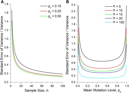
Dependence of the Standard Error of Variance Divided by the Variance on the Mean mtDNA Mutation Level p₀ and on the Sample Size n

(A) Dependence on the sample size n for three values of the mean mutation level.

(B) Dependence on the mean mutation level for a range of sample sizes. All standard error values are calculated for a Kimura distribution from Equations 11 and 2. All curves were calculated from Equations 11 and 2 with a value of b = 0.9. That b value was chosen as a simple value that was close to the b value calculated from the one human oocyte data set.^13,38

A practical approach would be to calculate the required sample size n via a general estimate based on the normal distribution approximation of Equation 6. One then needs to keep in mind that this will give a good prediction for the standard error of the variance in data sets with moderate mean mtDNA mutation levels (near 50%), but that data sets with high or low values of mean mutation level will have even higher relative standard errors of the variance, as illustrated in Figure 8B. The normal distribution method underestimates the standard error of variance for samples with high (>90%) or low (<10%) mean mutation level, so for calculating error bars for the measured variance, either the model-free method (Equations 2–4) or the Kimura model method (Equations 11 and 2) should be used.

Discussion

The calculation of mtDNA mutation level variance values from quite small sample sizes has been an accepted practice, although some have had concerns about this practice. We have addressed these concerns by developing the equations for calculating the standard error of variance measured from a sample of size n. We give three options for doing this calculation. The model-free method uses only the measured data and does not require any assumption of the form of the probability distribution from which the data are sampled. However, the model-free method does require the calculation of the fourth central moment of the data, and high-order moments such as this are difficult to estimate from data. The simplest option is to assume that the population follows a normal distribution, and in that case the standard error of the variance is quite simple to calculate. The difficulty with the normal distribution is that it is a poor description of the mutation level distribution at the high and low extremes and these are often the ranges of great practical interest. To deal with the details of the mtDNA mutation level distribution, we have developed the Kimura distribution³⁸ based on the theory of neutral genetic drift.⁴¹ Although the Kimura distribution is mathematically complicated, it is a reliable description of measured mtDNA mutation level distributions³⁸ and in this paper we have derived the standard error of variance for mutation level values drawn from a Kimura distribution.

Although the standard error of variance has not been used in this field, the standard error of the mean is, of course, common knowledge. We would argue that in general, assumptions about the reasonable number of samples to take in an experiment have been shaped by our familiarity with the standard error of the mean. However, a number of samples n that are quite sufficient for the accurate estimation of the mean value can be inadequate for the estimation of higher-order statistics, such as the variance. Comparisons of the confidence intervals for the mean values and for the variance values for both the normal distribution (Figure 1) and the Kimura distribution (Figures 2 and 3) illustrate this difference starkly. Although the confidence intervals for the mean are quite reasonably small for sample sizes of about 20, the corresponding confidence intervals for the variance measurements are disturbingly large at those samples sizes, making it extremely difficult to reliably measure small changes in variance. Because scientific conclusions are being made based on comparisons of these measured variances, it is critical that error bars for these variance measurements be reported and that reliable statistical tests for comparisons of variance measurements, such as the Levene test, should be used. Based on our Monte-Carlo results (Figures 6 and 7), a good rule of thumb for experimental design is that at moderate mean mutation levels (50%), a 2-fold or greater difference in normalized variance can be reliably detected by >30 measurements, while for low (10%) or high (90%) mean mutation levels, the number of measurements should be increased to 50 or more.

The standard error of variance is a critical tool for assessing the reliability of a variance measurement. With this new capability, we have reinterpreted the experimental data on the development of mtDNA mutation level variance in the female germline. In the mouse model, this reassessment shows that there is no support for the conclusion that the mutation level variance increases greatly during postnatal development (Figures 4A and 5), contrary to the previous interpretation of the data.¹⁰ The addition of the standard error of variance also shows that there is a clear difference between the mouse model and the human data, with humans having a far larger mtDNA mutation level variance than mice in both primary oocytes and offspring.

References

- 1.Chinnery P.F., Zwijnenburg P.J.G., Walker M., Howell N., Taylor R.W., Lightowlers R.N., Bindoff L., Turnbull D.M. Nonrandom tissue distribution of mutant mtDNA. Am. J. Med. Genet. 1999;85:498–501. [PubMed] [Google Scholar]
- 2.Frederiksen A.L., Andersen P.H., Kyvik K.O., Jeppesen T.D., Vissing J., Schwartz M. Tissue specific distribution of the 3243A->G mtDNA mutation. J. Med. Genet. 2006;43:671–677. doi: 10.1136/jmg.2005.039339. [DOI] [PMC free article] [PubMed] [Google Scholar]
- 3.Durham S.E., Bonilla E., Samuels D.C., DiMauro S., Chinnery P.F. Mitochondrial DNA copy number threshold in mtDNA depletion myopathy. Neurology. 2005;65:453–455. doi: 10.1212/01.wnl.0000171861.30277.88. [DOI] [PubMed] [Google Scholar]
- 4.Shoubridge E.A. Mitochondrial DNA diseases: Histological and cellular studies. J. Bioenerg. Biomembr. 1994;26:301–310. doi: 10.1007/BF00763101. [DOI] [PubMed] [Google Scholar]
- 5.Chinnery P.F., Thorburn D.R., Samuels D.C., White S.L., Dahl H.M., Turnbull D.M., Lightowlers R.N., Howell N. The inheritance of mitochondrial DNA heteroplasmy: Random drift, selection or both? Trends Genet. 2000;16:500–505. doi: 10.1016/s0168-9525(00)02120-x. [DOI] [PubMed] [Google Scholar]
- 6.Bredenoord A.L., Krumeich A., De Vries M.C., Dondorp W., De Wert G. Reproductive decision-making in the context of mitochondrial DNA disorders: Views and experiences of professionals. Clin. Genet. 2010;77:10–17. doi: 10.1111/j.1399-0004.2009.01312.x. [DOI] [PubMed] [Google Scholar]
- 7.Thorburn D.R., Dahl H.H.M. Mitochondrial disorders: Genetics, counseling, prenatal diagnosis and reproductive options. Am. J. Med. Genet. 2001;106:102–114. doi: 10.1002/ajmg.1380. [DOI] [PubMed] [Google Scholar]
- 8.Cao L.Q., Shitara H., Horii T., Nagao Y., Imai H., Abe K., Hara T., Hayashi J.I., Yonekawa H. The mitochondrial bottleneck occurs without reduction of mtDNA content in female mouse germ cells. Nat. Genet. 2007;39:386–390. doi: 10.1038/ng1970. [DOI] [PubMed] [Google Scholar]
- 9.Cree L.M., Samuels D.C., de Sousa Lopes S.C., Rajasimha H.K., Wonnapinij P., Mann J.R., Dahl H.H.M., Chinnery P.F. A reduction of mitochondrial DNA molecules during embryogenesis explains the rapid segregation of genotypes. Nat. Genet. 2008;40:249–254. doi: 10.1038/ng.2007.63. [DOI] [PubMed] [Google Scholar]
- 10.Wai T., Teoli D., Shoubridge E.A. The mitochondrial DNA genetic bottleneck results from replication of a subpopulation of genomes. Nat. Genet. 2008;40:1484–1488. doi: 10.1038/ng.258. [DOI] [PubMed] [Google Scholar]
- 11.Cao L.Q., Shitara H., Sugimoto M., Hayashi J.I., Abe K., Yonekawa H. New evidence confirms that the mitochondrial bottleneck is generated without reduction of mitochondrial DNA content in early primordial germ cells of mice. PLoS Genet. 2009;5:e1000756. doi: 10.1371/journal.pgen.1000756. [DOI] [PMC free article] [PubMed] [Google Scholar]
- 12.Jenuth J.P., Peterson A.C., Fu K., Shoubridge E.A. Random genetic drift in the female germline explains the rapid segregation of mammalian mitochondrial DNA. Nat. Genet. 1996;14:146–151. doi: 10.1038/ng1096-146. [DOI] [PubMed] [Google Scholar]
- 13.Brown D.T., Samuels D.C., Michael E.M., Turnbull D.M., Chinnery P.F. Random genetic drift determines the level of mutant mtDNA in human primary oocytes. Am. J. Hum. Genet. 2001;68:533–536. doi: 10.1086/318190. [DOI] [PMC free article] [PubMed] [Google Scholar]
- 14.Black G.C.M., Morten K., Laborde A., Poulton J. Leber's hereditary optic neuropathy: Heteroplasmy is likely to be significant in the expression of LHON in families with the 3460 ND1 mutation. Br. J. Ophthalmol. 1996;80:915–917. doi: 10.1136/bjo.80.10.915. [DOI] [PMC free article] [PubMed] [Google Scholar]
- 15.Carelli V., Ghelli A., Ratta M., Bacchilega E., Sangiorgi S., Mancini R., Leuzzi V., Cortelli P., Montagna P., Lugaresi E., Degli Esposti M. Leber's hereditary optic neuropathy: biochemical effect of 11778/ND4 and 3460/ND1 mutations and correlation with the mitochondrial genotype. Neurology. 1997;48:1623–1632. doi: 10.1212/wnl.48.6.1623. [DOI] [PubMed] [Google Scholar]
- 16.Enns G.M., Bai R.K., Beck A.E., Wong L.J. Molecular-clinical correlations in a family with variable tissue mitochondrial DNA T8993G mutant load. Mol. Genet. Metab. 2006;88:364–371. doi: 10.1016/j.ymgme.2006.02.001. [DOI] [PubMed] [Google Scholar]
- 17.Hammans S.R., Sweeney M.G., Brockington M., Lennox G.G., Lawton N.F., Kennedy C.R., Morgan-Hughes J.A., Harding A.E. The mitochondrial DNA transfer RNA(Lys)A—>G(8344) mutation and the syndrome of myoclonic epilepsy with ragged red fibres (MERRF). Relationship of clinical phenotype to proportion of mutant mitochondrial DNA. Brain. 1993;116:617–632. doi: 10.1093/brain/116.3.617. [DOI] [PubMed] [Google Scholar]
- 18.Harding A.E., Sweeney M.G., Govan G.G., Riordan-Eva P. Pedigree analysis in Leber hereditary optic neuropathy families with a pathogenic mtDNA mutation. Am. J. Hum. Genet. 1995;57:77–86. [PMC free article] [PubMed] [Google Scholar]
- 19.Houstěk J., Klement P., Hermanská J., Houstková H., Hansíková H., Van den Bogert C., Zeman J. Altered properties of mitochondrial ATP-synthase in patients with a T—>G mutation in the ATPase 6 (subunit a) gene at position 8993 of mtDNA. Biochim. Biophys. Acta. 1995;1271:349–357. doi: 10.1016/0925-4439(95)00063-a. [DOI] [PubMed] [Google Scholar]
- 20.Howell N., Xu M., Halvorson S., Bodis-Wollner I., Sherman J. A heteroplasmic LHON family: Tissue distribution and transmission of the 11778 mutation. Am. J. Hum. Genet. 1994;55:203–206. [PMC free article] [PubMed] [Google Scholar]
- 21.Hurvitz H., Naveh Y., Shoseyov D., Klar A., Shaag A., Elpeleg O. Transmission of the mitochondrial t8993c mutation in a new family. Am. J. Med. Genet. 2002;111:446–447. doi: 10.1002/ajmg.10613. [DOI] [PubMed] [Google Scholar]
- 22.Kaplanová V., Zeman J., Hansíková H., Cerná L., Houst'ková H., Misovicová N., Houstek J. Segregation pattern and biochemical effect of the G3460A mtDNA mutation in 27 members of LHON family. J. Neurol. Sci. 2004;223:149–155. doi: 10.1016/j.jns.2004.05.001. [DOI] [PubMed] [Google Scholar]
- 23.Larsson N.G., Tulinius M.H., Holme E., Oldfors A., Andersen O., Wahlström J., Aasly J. Segregation and manifestations of the mtDNA tRNA(Lys) A—>G(8344) mutation of myoclonus epilepsy and ragged-red fibers (MERRF) syndrome. Am. J. Hum. Genet. 1992;51:1201–1212. [PMC free article] [PubMed] [Google Scholar]
- 24.Lott M.T., Voljavec A.S., Wallace D.C. Variable genotype of Leber's hereditary optic neuropathy patients. Am. J. Ophthalmol. 1990;109:625–631. doi: 10.1016/s0002-9394(14)72429-8. [DOI] [PubMed] [Google Scholar]
- 25.Mak S.C., Chi C.S., Liu C.Y., Pang C.Y., Wei Y.H. Leigh syndrome associated with mitochondrial DNA 8993 T—>G mutation and ragged-red fibers. Pediatr. Neurol. 1996;15:72–75. doi: 10.1016/0887-8994(96)00126-9. [DOI] [PubMed] [Google Scholar]
- 26.Mäkelä-Bengs P., Suomalainen A., Majander A., Rapola J., Kalimo H., Nuutila A., Pihko H. Correlation between the clinical symptoms and the proportion of mitochondrial DNA carrying the 8993 point mutation in the NARP syndrome. Pediatr. Res. 1995;37:634–639. doi: 10.1203/00006450-199505000-00014. [DOI] [PubMed] [Google Scholar]
- 27.Phasukkijwatana N., Chuenkongkaew W.L., Suphavilai R., Luangtrakool K., Kunhapan B., Lertrit P. Transmission of heteroplasmic G11778A in extensive pedigrees of Thai Leber hereditary optic neuropathy. J. Hum. Genet. 2006;51:1110–1117. doi: 10.1007/s10038-006-0073-6. [DOI] [PubMed] [Google Scholar]
- 28.Piccolo G., Focher F., Verri A., Spadari S., Banfi P., Gerosa E., Mazzarello P. Myoclonus epilepsy and ragged-red fibers: Blood mitochondrial DNA heteroplasmy in affected and asymptomatic members of a family. Acta Neurol. Scand. 1993;88:406–409. doi: 10.1111/j.1600-0404.1993.tb05368.x. [DOI] [PubMed] [Google Scholar]
- 29.Porto F.B.O., Mack G., Sterboul M.J., Lewin P., Flament J., Sahel J., Dollfus H. Isolated late-onset cone-rod dystrophy revealing a familial neurogenic muscle weakness, ataxia, and retinitis pigmentosa syndrome with the T8993G mitochondrial mutation. Am. J. Ophthalmol. 2001;132:935–937. doi: 10.1016/s0002-9394(01)01187-4. [DOI] [PubMed] [Google Scholar]
- 30.Santorelli F.M., Shanske S., Jain K.D., Tick D., Schon E.A., DiMauro S. A T—>C mutation at nt 8993 of mitochondrial DNA in a child with Leigh syndrome. Neurology. 1994;44:972–974. doi: 10.1212/wnl.44.5.972. [DOI] [PubMed] [Google Scholar]
- 31.Tanaka A., Kiyosawa M., Mashima Y., Tokoro T. A family with Leber's hereditary optic neuropathy with mitochondrial DNA heteroplasmy related to disease expression. J. Neuroophthalmol. 1998;18:81–83. [PubMed] [Google Scholar]
- 32.Tatuch Y., Christodoulou J., Feigenbaum A., Clarke J.T.R., Wherret J., Smith C., Rudd N., Petrova-Benedict R., Robinson B.H. Heteroplasmic mtDNA mutation (T----G) at 8993 can cause Leigh disease when the percentage of abnormal mtDNA is high. Am. J. Hum. Genet. 1992;50:852–858. [PMC free article] [PubMed] [Google Scholar]
- 33.Uziel G., Moroni I., Lamantea E., Fratta G.M., Ciceri E., Carrara F., Zeviani M. Mitochondrial disease associated with the T8993G mutation of the mitochondrial ATPase 6 gene: A clinical, biochemical, and molecular study in six families. J. Neurol. Neurosurg. Psychiatry. 1997;63:16–22. doi: 10.1136/jnnp.63.1.16. [DOI] [PMC free article] [PubMed] [Google Scholar]
- 34.White S.L., Shanske S., McGill J.J., Mountain H., Geraghty M.T., DiMauro S., Dahl H.H.M., Thorburn D.R. Mitochondrial DNA mutations at nucleotide 8993 show a lack of tissue- or age-related variation. J. Inherit. Metab. Dis. 1999;22:899–914. doi: 10.1023/a:1005639407166. [DOI] [PubMed] [Google Scholar]
- 35.Wong L.J.C., Wong H., Liu A.Y. Intergenerational transmission of pathogenic heteroplasmic mitochondrial DNA. Genet. Med. 2002;4:78–83. doi: 10.1097/00125817-200203000-00005. [DOI] [PubMed] [Google Scholar]
- 36.Zhu D.P., Economou E.P., Antonarakis S.E., Maumenee I.H. Mitochondrial DNA mutation and heteroplasmy in type I Leber hereditary optic neuropathy. Am. J. Med. Genet. 1992;42:173–179. doi: 10.1002/ajmg.1320420208. [DOI] [PubMed] [Google Scholar]
- 37.Wilks S.S. Wiley; New York: 1962. Mathematical Statistics. [Google Scholar]
- 38.Wonnapinij P., Chinnery P.F., Samuels D.C. The distribution of mitochondrial DNA heteroplasmy due to random genetic drift. Am. J. Hum. Genet. 2008;83:582–593. doi: 10.1016/j.ajhg.2008.10.007. [DOI] [PMC free article] [PubMed] [Google Scholar]
- 39.Sheskin D.J. Chapman & Hall / CRC; Boca Raton, FL: 2007. Handbook of Parametric and Nonparametric Statistical Procedures. [Google Scholar]
- 40.Dodge Y., Rousson V. The complications of the fourth central moment. Am. Stat. 1999;53:267–269. [Google Scholar]
- 41.Kimura M. Solution of a process of random genetic drift with a continuous model. Proc. Natl. Acad. Sci. USA. 1955;41:144–150. doi: 10.1073/pnas.41.3.144. [DOI] [PMC free article] [PubMed] [Google Scholar]
- 42.Charlesworth B. Fundamental concepts in genetics: Effective population size and patterns of molecular evolution and variation. Nat. Rev. Genet. 2009;10:195–205. doi: 10.1038/nrg2526. [DOI] [PubMed] [Google Scholar]
- 43.Wright S. Statistical genetics and evolution. Bull. Am. Math. Soc. 1942;48:223–246. [Google Scholar]
- 44.Wright S. Evolution in Mendelian populations (reprinted from Genetics, vol 16, pg 97-159, 1931) Bull. Math. Biol. 1990;52:241–295. doi: 10.1007/BF02459575. [DOI] [PubMed] [Google Scholar]
- 45.Solignac M., Genermont J., Monnerot M., Mounolou J.C. Genetics of mitochondria in Drosophila—mtDNA inheritance in heteroplasmic strains of Drosophila-Mauritiana. Mol. Gen. Genet. 1984;197:183–188. [Google Scholar]
- 46.Rajasimha H.K., Chinnery P.F., Samuels D.C. Selection against pathogenic mtDNA mutations in a stem cell population leads to the loss of the 3243A—>G mutation in blood. Am. J. Hum. Genet. 2008;82:333–343. doi: 10.1016/j.ajhg.2007.10.007. [DOI] [PMC free article] [PubMed] [Google Scholar]