Model-Based Global Analysis of Heterogeneous Experimental Data Using gfit

Summary

Regression analysis is indispensible for quantitative understanding of biological systems and for developing accurate computational models. By applying regression analysis, one can validate models and quantify components of the system, including ones that cannot be observed directly. Global (simultaneous) analysis of all experimental data available for the system produces the most informative results. To quantify components of a complex system, the dataset needs to contain experiments of different types performed under a broad range of conditions. However, heterogeneity of such datasets complicates implementation of the global analysis. Computational models continuously evolve to include new knowledge and to account for novel experimental data, creating the demand for flexible and efficient analysis procedures. To address these problems, we have developed gfit software to globally analyze many types of experiments, to validate computational models, and to extract maximum information from the available experimental data.

1. Introduction

Computational models play increasingly important roles in biology. Constructing a model that accurately represents the mechanism of a system, reliably simulates its behavior, and has well-defined parameter values is the ultimate goal of many research projects. Models are used for interpreting experimental observations, testing hypotheses, integrating knowledge, discovering components responsible for certain behavior, designing more informative experiments, and making quantitative predictions (1). Remarkably, computational models act both as tools for studying biology and as representations of the resulting knowledge. Indeed, quantitative mechanistic information incorporated into a model allows it to make predictions outside the domain of existing observations.

The focus of this chapter is on understanding experimental data and extracting useful information from it. The role of a model in this process is to postulate a relationship between conditions of experiments and the observed results. Using regression analysis, different models can be tested for their ability to explain the experimental observations, and their parameters can be estimated. Thus, regression analysis ties together models and data, validating the former and extracting information from the latter (2, 3).

Unfortunately, practical application of this procedure to biological systems can be complicated. As will be shown in this chapter, even relatively simple models may contain too many parameters to estimate based on a single experiment of any type. Therefore, to test whether the model is consistent with the data and to determine its parameters, data from multiple experiments need to be analyzed globally, while applying all known constraints to the values of parameters (4).

In this chapter, we discuss the challenges associated with practical application of regression analysis to biological systems. The problems we describe are exacerbated in complex models and experimental designs, and thus are especially frustrating for quantitative biologists. We describe our software, gfit, which helps to overcome these problems and illustrate its utility with three biological systems of increasing complexity.

1.1. Regression Analysis

Regression analysis includes a range of methods for establishing a model that accurately represents a system and makes accurate predictions of its behavior. The specific tasks include searching for optimal parameter values, testing whether the model agrees with experimental data, estimating parameter confidence intervals, testing whether more experimental data are needed, detecting outlier points, and selecting the preferred model from two possible ones. In regression analysis, model F is defined as a quantitative relationship between experimental measurements (dependent variables) ϒ and experiment conditions (independent variables) C

$$\mathit{\Upsilon }=F(C,x)+\epsilon$$ (1)

where x is a vector of model parameters (variables affecting behavior of the system that cannot be controlled or directly observed during experiment), and ε is a set of measurement errors (see Note 1) (5).

Goodness of fit, the closeness of model simulations to the measurements, is quantified by objective function S(x). The most commonly used objective function is a sum of squared residuals (see Note 2),

$$S(\mathit{\text{x}})=\sum _{i=1}^N{\left[{\mathit{\text{ϒ}}}_i-\mathit{\text{F}}({\mathit{\text{C}}}_i,\mathit{\text{x}})\right]}^2$$ (2)

or, in case of nonuniformly distributed ε, a weighted sum of squared residuals

$$S(\mathit{\text{x}})=\sum _{i=1}^N{\left[\frac{{\mathit{\text{ϒ}}}_i-\mathit{\text{F}}({\mathit{\text{C}}}_i,\mathit{\text{x}})}{{\sigma }_i}\right]}^2,\text{Where}{\sigma }_i\text{is a standard deviation of}{\epsilon }_i$$ (3)

Curve fitting is a problem of finding parameters x that produce the best fit, that is minimize the objective function:

$$\underset{\text{X}}{\text{min}}S(\mathit{\text{x}}).$$ (4)

Curve fitting is an optimization problem, performed by optimization engines. Many tasks of regression analysis are based on curve fitting.

1.2. Applying Regression Analysis to Experimental Data

One common obstacle to broader application of regression analysis to biological problems is failure of many models to directly simulate the experimentally observed variable. For example, a typical system model may simulate concentrations of reacting species, values that are rarely observed in an experiment directly. One way of addressing this discrepancy is to convert measured values into the type simulated by the model. However, such conversions often introduce statistical errors and are not always possible. The better solution is to simulate exactly the same value type as measured in the experiment. To achieve that, separate experiment models may be required. Experiment models use the system model to simulate the system's response to manipulations and the experimentally measured signal (see Fig. 1). The approach of separating system models and experiment models is used in Virtual Cell software (6).

Fig. 1.

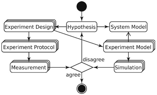
Application of scientific method to quantitative biology. Mechanistic Hypothesis about a biological system leads to a System Model, a quantitative description of system components and their interactions. To test the Hypothesis, the system is treated in a controlled manner and its behavior is measured. The ideas, assumptions, and, possibly, hypotheses involved in the treatment are parts of Experiment Design. The Measurement obtained by following the Experiment Protocol is compared with Simulation. To make the comparison meaningful, all Simulations need to have same physical meaning and dimensionality as their corresponding Measurements. Therefore, an Experiment Model, an in silico counterpart of Experiment Protocol, is derived from each Experiment Design. Experiment Models interacting with the System Model produce Simulations that are quantitatively compared with the Measurements.

A curve fitting procedure for a heterogeneous dataset can be quite complex and require extensive communication between its entities, i.e., model, optimization engine, experiment conditions, measurements, parameters, and constraints (see Fig. 2A). Before a search for optimal parameter values can begin, the data for each experiment has to be examined:

Fig. 2.

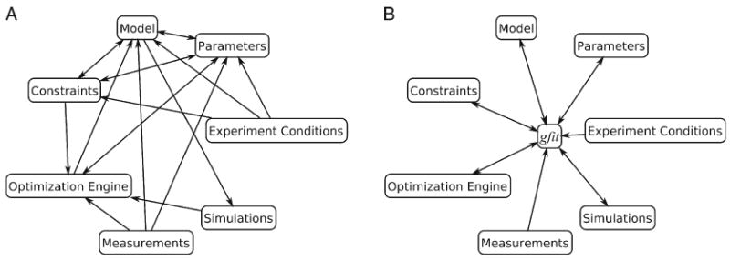
Components of regression analysis. Arrows indicate information flow between components. (A) Analysis procedure requires extensive interactions between components. (B) To streamline the procedure, gfit mediates all interactions between components.

• – To determine which variables need to be simulated and their sizes

• – To check that the data required for the simulation has been provided

• – To check against constraints on variable dimensions and values imposed by the model

• – To determine what parameters can be estimated and to choose their starting values

Once the data have been examined, the optimization procedure can be initiated by passing a vector of starting parameter values to the optimization engine. Depending on the engine type, parameter constraints can be also provided. The engine conducts optimization by repeatedly changing parameters and recalculating the objective function on the basis of experimental measurements and simulations. To simulate each experiment, the input data for the model has to be assembled from applicable optimization parameters and experiment conditions. The input data also have to be checked against the constraints, since not all of them can be enforced by optimization engines. After simulating all experiments, the appropriate objective function can be computed and used by optimization engine to determine the direction of the search.

Curve fitting procedure follows complicated rules that depend on the computational model, experimental data, and optimization engine. In addition, parameter constraints need to reflect various considerations related to the research project. These factors make the analysis procedure not only complex, but also highly variable, making design and maintenance of project-specific software prohibitively expensive. Fortunately, the patterns of data flow during regression analysis are largely independent of the system under investigation. This fact allowed us to design software that solves the analysis problem generally and for any model type.

1.3. Design of gfit

The purpose of gfit is connecting models with various types of experimental data. First, it simplifies the model's task of directly simulating experimentally observable variables. Second, during regression analysis, gfit maintains communications between the analysis components, acting as a mediator (see Fig. 2B). Third, by defining standard application interfaces for models, optimization engines, objective functions, and other entities, it facilitates customization of the analysis procedure.

Of all components, application interfaces of models represent the biggest problem. Almost every step of regression analysis procedure depends on what information is required and produced by the model. Yet, every model has different inputs and outputs. To be able to perform regression analysis with any kind of computational model, gfit uses a metadata approach. Any model used by gfit is expected to have an attached Model Description (see Note 3) defining its inputs and outputs as sets of variables (see Note 4). More information about Model Descriptions is provided later in this chapter. Once the rules for performing simulations with the model are known, the analysis process becomes more straightforward and independent of the model type (Fig. 3).

Fig. 3.

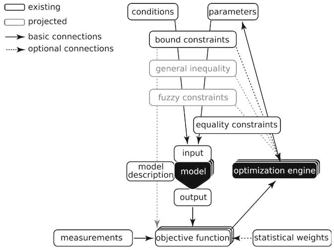
Flow of information through regression analysis components. Communications between the components are controlled by gfit according to Model Description. During simulation of each experiment, independent variables from the experiment conditions and parameters are tested against constraints and combined into model input data. The input received by the model is guaranteed to be valid and to contain sufficient information for the simulation. Combining conditions with parameters keeps the model agnostic about the purpose of the simulation. Size of variables in model output depends on the input. The dependence is defined in Model Description and used by gfit to provide the input that will result in model output directly comparable with the measured variables for that experiment.

Regression analysis is a complicated process with many pitfalls. gfit strives to provide information that can help researchers avoid mistakes related to the analysis. In the protocols that follow, the reader will build simple models and use the existing models and experimental data for parameter estimation.

2. Materials

2.1. Software Requirements

1. Version 6.5 or later of MATLAB (Mathworks, Natick, MA), a common science and engineering computing software, is required for running simulations.

2. MATLAB Optimization Toolbox (Mathworks) is required for regression analysis.

2.2. Installation of gfit

1. Download the latest version of gfit from http://gfit.sourceforge.net. The zip-archive contains gfit.jar library and other files required for interaction of gfit with MATLAB.

2. Unzip the file to a convenient location on your hard disk. For this chapter we will assume location C:/. Folder C:/Mgfit will be created.

3. Start MATLAB.

4. Change MATLAB's current directory to C:/Mgfit.

5. To start installation, type mgfit in MATLAB's command line and press Enter.

6. Respond Yes to the query about adding C:/Mgfit to MATLAB's path.

7. Restart MATLAB if requested.

8. After installation, the same command, mgfit, will bring up gfit user interface window.

2.3. Installation of rsys Library

rsys library is used for solving ODEs for mass-action reaction systems, as described in Subheading 3.3.

1. Download the latest version of rsys for your operating system from http://gfit.sourceforge.net.

2. Unzip the file and put the library file anywhere on the MATLAB path. For example, to C:/Mgfit folder.

2.4. Data and Models

A zip archive containing all model and data files mentioned in this chapter can be downloaded from http://gfit.sourceforge.net. The data files included are in tab/newline-delimited format. These files can be opened in a text editor, but it is more convenient to view them in a spreadsheet. Please check the readme.txt file for the most current information.

3. Using gfit: Examples

3.1 Simple Model Example: Equilibrium Binding

In this section, we will create a model for equilibrium binding of a protein, E, to a ligand, L, (Eq. 5) and use it for analysis of experimental data. This analysis is quite simple and can be accomplished with many existing programs (including commonly used spreadsheet applications). We will use it to illustrate the principles of data analysis and model validation used by gfit, and later apply them to more interesting examples.

$$E+L\stackrel{K_D}{\rightleftharpoons }EL,\text{where}{K}_{\text{D}}=\frac{\left[E\right]\left[L\right]}{\left[EL\right]}$$ (5)

If only total concentrations of E and L are known, E_T = [E] + [EL] and [L_T] = [L] + [EL], equilibrium concentration of the complex can be written as

$$\left[EL\right]=\frac{K_{\text{D}}+E_{\text{T}}+L_{\text{T}}-\sqrt{{\left(K_{\text{D}}+E_{\text{T}}+L_{\text{T}}\right)}^2-4E_{\text{T}}{L}_{\text{T}}}}{2}$$ (6)

3.1.1. Create Standalone Model

1. Open MATLAB editor by typing edit in the command line. Editor window will appear.

2. Add the code shown in Listing 1 and save the file as eq_binding.m in C:/Mgfit/Models folder.

Listing 1. MATLAB function simulating binding equilibrium.

1. function signal = eq_binding(Et, Lt, Kd)

2. %simulate equilibrium binding E + L <=> EL

3. EL = (Kd + Et + Lt - sqrt((Kd + Et + Lt). ˆ2 - 4 * Et.* Lt))/2;

4. signal = EL;

Steps 1 and 2 create a MATLAB m-file function. Line 1 contains MATLAB keyword function followed by the name of the output variable signal, followed by the name of the function, eq_binding, and a list of input variables (Et, Lt, Kd). Line 2 is a comment, marked in MATLAB by the % character. Line 3 performs the calculation according to Eq. 6. Line 4 assigns the calculated, [EL], to the output variable.

3.1.2. Perform Simulation

The model we created has three input variables and one output variable. To perform a simulation, we need to supply values for input variables and store the result in the output variable. Variables in MATLAB (and in gfit) can contain a single value or arrays of numbers. The arrays may have 0, 1, or many dimensions. 0D array, scalar, stores a single number; 1D array, stores a vector of numbers; 2D array contains a matrix, etc. Models can take advantage of this fact. For example, our model can accept vectors of Et and Lt concentration and simulate an entire titration curve in one call. We will use the model in Listing 1 to simulate different experiments.

3.1.3. Simulate Titration Curves

1. Simulate and plot a titration curve for Lt changing from 0 to 50

   Lt = 0:50; EL = eq_binding(1, Lt, 5); plot(Lt, EL)

2. Simulate and plot a titration curve for Et changing from 0 to 20

   Et = 1:20; EL = eq_binding(Et, 10, 5); plot(Et, EL)

   The model is flexible in that it can simulate experiments with different numbers of measurements (20 or 50) and with different combinations of variables that change and remain constant. However, if we did not know how input variables were used inside the model, it would be easy to call the model with illegal variables. For example, the following command will produce an error, because the size of Et vector is not equal to the size of Lt vector.

   Et = 1:20; Lt = 0:50; EL = eq_binding (Et, Lt, 5);

As well, mistakenly supplying negative values for the input parameters will produce a warning and a meaningless simulation result. Although we can keep track of correct variable sizes and values when manually executing a simple model, this task becomes tedious if many different experiments have to be simulated by a complex model. To create a connection between experimental data and a model that is practically useful, there has to be a method for automatically tracking the requirements of the model and for reconciling these requirements with existing experimental data. gfit learns about the requirement of the model and its expected output by reading the associated user generated Model Description (see Note 3).

3.1.4. Create gfit Model Description

1. Insert lines 3–13 into previously created eq_binding.m, as shown in Listing 2.

2. Add variable signal to the list of inputs.

   MATLAB m-files with a tag as on line 3 are recognized by gfit as models. Lines 3–13 are occupied by Model Description. Note that each of the lines starts from character %, a comment in MATLAB language. Therefore, Model Description is ignored by MATLAB and the meaning of the original program is not changed. Model Description is used by gfit to ensure that the model always receives legitimate input variables and to interpret experimental data that belongs to the model.

Listing 2. gfit model for binding equilibrium.

1	function signal = eq_binding(Et, Lt, Kd, signal)
2	%simulate equilibrium binding E + L <=> EL
3	%<gfitModelDescription version=“100”>
4	%variable	type	minVal
5	% Et	free	0
6	% Lt	independent	0
7	% Kd	para	0
8	% signal	dependent	()
9	%
10	%variable	size	plotVs
11	% Et	Lt	()
12	% signal	Lt	Lt
13	%</gfitModelDescription>
14	EL = (Kd + Et + Lt - sqrt((Kd + Et + Lt). ˆ2 - 4 * Et.* Lt))/2;
15	signal = EL;

The information in Model Description is organized in a tabular fashion. Any number of tables can be present. Tables in Model Description are space/tab/newline-delimited. Rows in each table should contain same number of elements. However, if an element needs to be empty (as in minVal of signal variable), an empty pair of brackets ((), [], ‘’, or “”) can be used. Brackets should also surround multiword elements.

The first table (lines 4–8) should list all model I/O variables in the same order as in the input list of the function. The first column of every table contains variable names. The second column of the first table defines variable types. Type free for variable Et means that its value could either be known precisely and supplied with the experiment conditions, or not known and appear as one of the optimization parameters. Variable Lt is independent, meaning that its value should always be known exactly and appear in the experimental data. Variable Kd has para type and is sought as an optimization parameter. Variable signal has dependent type and therefore is expected to be calculated by the model.

The Model Description is also used to set bound limits on the input variables. Column three of the first table, (minVal) specifies the minimum value of zero for all variables except signal, which is dependent and cannot have its value constrained. This has been included in the first table but can also be placed in a separate table.

In this example, the size of variables is set in the second table of Model Description (lines 10–12). The length of Et variable vector is set equal to the length of Lt as required by the model. It also sets the length of signal produced by the model to have the length of Lt. Since the size of the output variable must be known by gfit, the latter expression guarantees that the results are equal to a known length. The table also states (line 12, in the third column-plotVs) that signal should be plotted versus Lt.

3.1.5. Import Data into gfit

1. Start gfit by typing mgfit in MATLAB command line. gfit window will appear.

2. Select eq_binding.m model by choosing menu Model →Pick Model. The name of the model will appear in the model field.

3. Arrange data for two experiments in a spreadsheet application as shown in Fig. 4A. Names of the experiments should appear in the top line of the data block. First experiment Titration one contains two variables Lt and Et having equal size. Second experiment, Titration two, contains only the independent variable, Lt, required by the model. Note that variables Lt in experiments one and two have different sizes.

4. To transfer data to gfit, select both experiments in the spreadsheet and copy it into the clipboard. Names of experiments should appear in the top row of the selected block.

5. In gfit window, choose menu Data→Paste-add Data. gfit recognizes tab/newline-delimited data stored in clipboard and checks it against the requirements of Model Description to assure that it can be used with the current model. If there is an inconsistency between data and the requirements of the Model Description, an error message will appear.

Fig. 4.

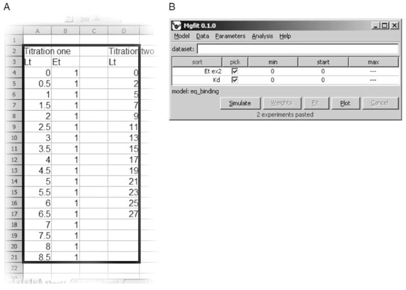
gfit imports experimental data from a spreadsheet. (A) Spreadsheet containing two experiments–Titration one and Titration two. Black rectangle shows the cells to be selected, copied, and imported to gfit. (B) Once the data are imported, gfit user interface shows model parameters.

Once the data is acquired by gfit, it generates parameters for all para variables and for every free model variable in the model that is missing in the experimental data (Fig. 4B). Parameters are generated based on the input variables defined in Model Description.

During simulation of an experiment, input variables draw their values either from the supplied experimental data, or from current values of parameters. In gfit, parameters and input variables have a many-to-many relationship. When simulating different experiments, a variable containing an array of numbers can collect its values from many parameters. One parameter can be also connected to multiple variables as long as the variables have the same physical units (discussed below).

Linkage of parameters to different variables can be adjusted through gfit parameter table in the user interface (Fig. 4B). For every parameter, the table shows its name, optimization flag (pick), low bound constraint (smallest value allowed), start (current) value, and upper bound constraint. Parameters in the table can be sorted by several criteria. To switch between different sorting methods, click sort parameter table header button. All parameters can be selected or deselected for optimization (discussed below) by clicking on pick button. Bound constraints for each parameter are set based on the variable's constraints in the Model Description. The valid interval of constraints can be only reduced through the user interface. For example, minimal value for K_D can be changed to 1.0, but not to −1.0.

3.1.6. Simulate with gfit

1. Set parameter Et ex2 to 15.0 and parameter Kd to 1.

2. To perform simulation click on Simulate button.

3. Click on button Plot. A plot will appear.

The model we created can be conveniently used for simulating equilibrium concentration of EL complex under different experiment conditions. Unfortunately, concentration of a complex is seldom measured directly in an experiment. In the simplest case, experimentally observed values are proportional to [EL]. To avoid transformation of the data (even a linear one) prior to analysis, the model needs to simulate the measured signal.

3.1.7. Refine Model

1. To simulate the signal observed in a real experiment (e.g., binding induced change of fluorescence), introduce two more variables, signal gain, gain, and signal background, c. Assume the signal to be proportional to [EL] with an offset.

2. Add more columns to the first table of Model Description to set default starting values of parameters, physical units, and human-readable descriptions of model variables. Resulting model is shown in Listing 3.

Listing 3. Updated gfit model for binding equilibrium.

1	function signal = eq_binding(Et, Lt, Kd, signal, gain, c)
2	%binding equilibrium E + L < = > EL; simulate signal proportional to [EL]
3	%<gfitModelDescription version=“100”>
4	%variable	type	minVal	startVal	unit	comment
5	% Et	()	0	1	uM	‘total concentration of E’
6	% Lt	independent	0	1	uM	‘total concentration of L’
7	% Kd	para	0	0.1	uM	‘dissociation constant’
8	% signal	dependent	()	()	()	‘complex formation’
9	% gain	para	()	1	()	‘signal gain’
10	% c	para	()	0	()	‘signal background’
11	%
12	%variable	size	plotVs
13	% Et	Lt	()
14	% signal	Lt	Lt
15	%</gfitModelDescription>
16	EL = (Kd + Et + Lt - sqrt((Kd + Et + Lt). ˆ2 - 4 * Et.* Lt))/2;
17	signal = c + gain * EL;

These changes make this model more flexible because it can now be used for any experiment that measures a value proportional to the equilibrium concentration of the complex. Parameters by default take more reasonable starting values. Human readable variable descriptions appear when mouse cursor hovers over a name in the parameter table. Units prevent mixing incompatible variables in the same parameter.

3.1.8. Fit Data

1. From the data archive, open file eq_binding_data_fig5.txt in a text editor. The file contains data for one experiment, select and copy its entire contents.

2. In gfit interface, select the updated model and import the data into gfit.

3. To view the imported data click Plot.

4. Click Fit. Optimization engine will search parameter space for the best fit, and will display the optimized values and their confidence intervals (Fig. 5) (see Notes 5, 6, and 7).

5. To view fitted data click Plot.

Fig. 5.

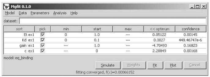
Fitting the results of a fluorimetric titration experiment. The interface shows optimal values for each parameter and their confidence intervals.

In this section, we have created a regular MATLAB m-file and added a gfit Model Description to it, which allowed us to connect it with experimental data to perform simulation and fitting. In the following sections, we will apply this technique to more complex biological systems.

3.2. More Complex Example: Equilibrium Binding to a Polymer

The model created in the previous section can be used for studying relatively simple systems where binding properties are characterized only by the dissociation constant. However, binding processes are often more complex and characterized by multiple parameters. Binding of proteins to discrete positions on a linear lattice (DNA, RNA, microtubules, and microfilaments) plays important roles in many biological processes. In this section, we will discuss binding of the helicase from hepatitis C virus to single-stranded (ss) DNA substrates. The experimental data were obtained by titrating a constant concentration of the helicase with oligonucleotides of different lengths while monitoring the reduction of intrinsic fluorescence of the helicase caused by ssDNA binding (7). With this example we take regression analysis a step further and globally fit many titration curves to quantify helicase properties that are not apparent from any single experiment.

The model of equilibrium binding to a lattice, in addition to concentrations and the dissociation constant, uses parameters related to the geometry of the molecules, namely lattice length N, protein's minimal binding site (M, number of lattice units interacting with the protein), and protein's occlusion site (S, number of lattice units from which one protein molecule excludes the others) (Fig. 6A). The model assumes noncooperative and sequence-independent binding. Since the K_D observed in lattice binding experiments changes with the lattice length, the model uses a more fundamental microscopic dissociation constant, $K_{\text{D}}^0$, defined as the dissociation constant observed with lattice of length M. Thus, variables $K_{\text{D}}^0$, M, and S keep same values in all experiments.

Fig. 6.

Binding of proteins to lattices depends on their geometry. (A) Protein geometry parameters are minimal binding site, M, and occlusion site, S. (B) If lattice length, N < M, binding free energy is approximately proportional to N. (C) If N > M, the observed K_D is inversely proportional to the number of alternative binding configurations, N − M + 1. (D) If more than one protein can bind to a lattice molecule, N ≥S + M, binding configurations for all possible numbers of bound proteins have to be considered.

The model calculates concentration of bound protein, E_B, from total protein concentration, E_T, total concentration of lattice, L_T, and N. Depending on relative values of M, S, and N, three cases can be considered. If lattice is shorter than the minimal binding site (Fig. 6B), N < M, and assuming equal contribution of each lattice unit to the binding free energy, the binding can be described by Eq. 6, where the observed dissociation constant

$$K_D=K_D^{0(N/M)}{\xi }^{(1-N/M)},\text{where}\xi \text{is a concentration unit conversion factor}.$$ (7)

For longer lattices that can accommodate only one protein molecule (Fig. 6C), M ≤ N < 2S, the observed dissociation constant is inversely proportional to the number of distinct positions the protein can occupy.

$$K_{\text{D}}=\frac{K_{\text{D}}^0}{N-M+1}$$ (8)

If multiple proteins can bind to a single lattice molecule, Eq. 6 can no longer be used, and the extent of binding has to be calculated by numerically solving Eq. 9 (8). Alternatively, if the number of proteins bound to a lattice is large, a lower order equation can provide accurate results (9).

$$\frac{E_{\text{B}}}{L_{\text{T}}}=\frac{{\sum }_{i=0}^{L_{\text{max}}}i{\mathrm{\Omega }}_i{\left(\frac{E_{\text{T}}-E_{\text{B}}}{K_{\text{D}}^0}\right)}^i}{{\sum }_{i=0}^{L_{\text{max}}}{\mathrm{\Omega }}_i{\left(\frac{E_{\text{T}}-E_{\text{B}}}{K_{\text{D}}^0}\right)}^i},\text{where}{\mathrm{\Omega }}_i=\frac{\left(N-iS+i\right)!}{\left(N-iS\right)!i!}$$ (9)

Although apparent dissociation constant, K_D, can be estimated on the basis of a single titration experiment, true $K_{\text{D}}^0$ cannot be determined without prior knowledge of M and S. All three parameters can be determined simultaneously by globally fitting titration curves for many ssDNA substrates of different lengths.

The model for lattice binding lattice_binding_v1.m, provided in the data archive, follows a similar pattern as previously created eq_binding.m model. Both models start with Model Description. We will now test whether the model is consistent with the observed results, estimate the parameters, and determine their confidence intervals.

3.2.1. Import Titration Data for Global Analysis

1. Start gfit and choose model lattice_binding_v1.m.

2. Open file lattice_binding_data.txt in a spreadsheet. The file contains data for nine titration experiments. As before, the top row contains only names of experiments with variable names and values appearing below (see Note 8).

3. Select and copy entire dataset. Make sure that selection starts at experiment name row and no values on the bottom are left out.

4. Choose menu Data→Paste-add Data to import data to gfit. The parameters generated for the dataset will appear. View data by clicking button Plot.

3.2.2. Fit the Data

1. Make sure that all parameters are selected for optimization and click button Fit. Because of the larger number of parameters and more involved computation, fitting may take a couple of minutes to complete.

2. Plot the fitted data. The fit does not match the data. Notice, however, that unlike the data, all fitted curves start from the same value. This happened because same value of f 0 parameter was used for all experiments.

3. Right-click on the name of f0 parameter and choose menu Separate Elements. Parameter f0 separated into nine parameters, one for each experiment. Also separate elements of parameter fg, because the gain of the signal is also known to vary between experiments.

4. Click button Fit.

Using this model and dataset, gfit is expected to produce a good fit at the first attempt (Figs. 7 and 8). However, this result is not typical. In our experience with other models, local optimization algorithms seldom find the global minimum in the first attempt. This highlights the importance of global optimization methods (10, 11). Generally, finding a global minimum of a nonlinear problem is unattainable within finite time. Nevertheless, even if a good fit has been found, it is advisable to search the parameter space for alternative minima. Discovering distinct sets of parameters that produce “as good,” or “nearly as good” fits is important to diagnose overparameterized models or insufficient amount of experimental observations.

Fig. 7.

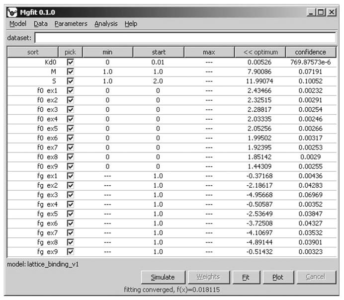
Results of global fitting of nine equilibrium titration experiments. The interface shows a table of 21 parameters. Three parameters, Kd0, M, and S, were globally applied to all experiments, while each of the others were used in one experiment only. For example, parameter f0 ex3 was used in experiment 3 only. Optimization started with parameter values displayed in column start, and arrived to the optimal values displayed in column optimum. Column confidence shows parameter standard errors (68% confidence intervals) estimated using asymptotic method.

Fig. 8.

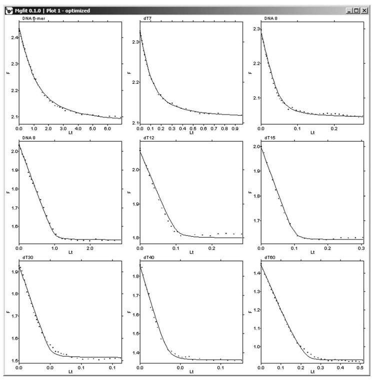
Plots of nine globally fitted titration experiments. In each titration, increasing concentrations of ssDNA were added to the constant concentration of helicase. Concentrations of helicase as well as lengths of ssDNA were different in each titration. Binding to DNA reduced the intrinsic fluorescence of the helicase. Experimental measurements of fluorescence are shown as dots. Results of the simulation are shown as solid lines.

The method currently used by gfit for exploring parameter space is random restart. This simple method is implemented as a “globalizer” on top of the existing local optimization engine. Random restart repeatedly reinitiates local optimization with a randomly chosen set of parameters. The new starting parameter values are picked from a uniform distribution for doubly-constrained parameters, from a truncated normal distribution for singly-constrained parameters, and from a normal distribution for the unconstrained ones. Random restart procedure is implemented without a defined termination condition. It is supposed to be interrupted by the user.

3.2.3. Search for Global Minimum

1. Choose menu Analysis→Random Restart (see Note 9).

2. Allow the program to perform a few hundred optimizations and interrupt it by clicking button Cancel. The best found parameter values appear in the right column of the parameter table.

3. To check the goodness of fit visually, copy best found parameter values to the start column by clicking the table header button ≪value, click button Simulate, then button Plot (see Note 10).

More generally, the following rule-of-thumb procedure can be used to decide if the random restart search should be continued.

3.2.4. When Should Random Restart be Terminated?

1. With random restart running or terminated, open most recent file C:/Mgfit/Temp/Optim_nnn.txt in a simple text editor (see Note 9).

2. Select and copy entire contents of the file and paste it into a spreadsheet application. Now each row of the spreadsheet contains a set of optimized parameters, while the first column contains the values of objective function. Parameter sets appear in the order they were calculated.

3. Sort parameter sets by their objective function. The best fitting parameter set is now at the top row of the table.

4. Examine the better fitting parameter sets. Identify a group of better fitting sets with similar goodness of fit values starting from the top row.

   1. If the group is small, the search is worth continuing.

   2. If the group is large and at least some of the parameters have significantly different values, the data does not sufficiently constrain model parameters. Additional experiments may be needed.

   3. If the group is large and parameter values are similar between different sets, the group is probably in the vicinity of the global minimum of the problem.

3.3. Advanced Example: Kinetic Mechanism of Clamp Assembly on DNA

In this section, we describe modeling and analysis of a kinetic pathway responsible for loading sliding clamp proteins onto DNA during replication initiation. The clamp, PCNA, encircles DNA and binds to DNA polymerase, conferring processivity to the replication complex. PCNA is loaded onto DNA by the heteropentameric clamp loader protein, RFC, in a process that involves ATP binding and hydrolysis and conformational changes of the proteins (Fig. 9A) (12). Although the process has been extensively studied, understanding at the quantitative level is incomplete. Properties of individual species and reactions involved in this process are difficult to determine because almost any measurement technique is affected by a combination of many simultaneously occurring reactions. Computational modeling in conjunction with regression analysis provides a feasible solution to this complex problem.

Fig. 9.

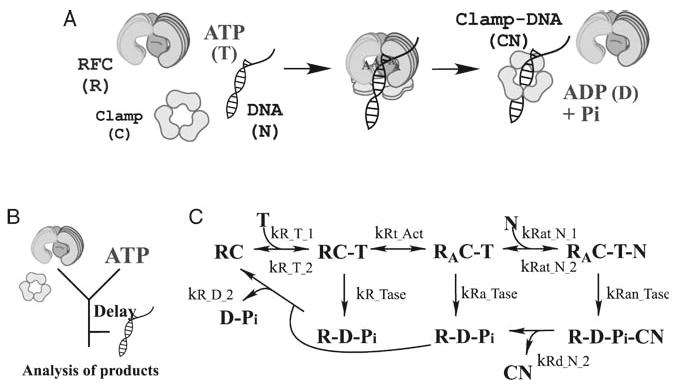
Mechanism of clamp loading on DNA. (A) Clamp loader protein, RFC, catalyzes assembly of circular PCNA clamps onto primed DNA in a reaction driven by ATP binding and hydrolysis. (B) Design of ATPase experiments, with initial mixing of RFC and PCNA with ATP, followed by varying delay times, mixing with DNA, and measurement of product kinetics. (C) Simplified clamp loading reaction scheme. RFC (in the presence of PCNA; RC) binds ATP (T). The ternary complex undergoes an activation step (RA) before DNA (N) binding, rapid ATP hydrolysis and dissociation from the clamp-DNA complex (CN).

Currently we are building, validating, and refining a mechanistic model of the process that can resolve many species and quantify the rates of individual reactions that may not be observed experimentally. A simplified reaction scheme, the first iteration of modeling process, is shown in Fig. 9C. The challenge of estimating the rates of many individual reactions can be addressed by monitoring the process from different perspectives. As noted earlier, each measurement is a function of many or all of the rates in the process; however, measurements from different perspectives are likely to be affected in distinct ways by individual reaction rates. Therefore, taken together, multiple measurements of presteady-state kinetics monitored by a few different methods can provide sufficient constraints to the parameters of the model.

Results of global regression analysis of data from two types of presteady-state experiments, one measuring ATP hydrolysis and the other phosphate (Pi) release by RFC protein, are shown in Figs. 10 and 11. ATP hydrolysis was monitored by a radiometric assay measuring formation of ³²P-ADP over time from ³²P-ATP, and Pi release was monitored by the change in fluorescence of a reporter, Pi Binding Protein, on binding the Pi released by RFC following ATP hydrolysis. Salient features of the experimental design in both cases are (Fig. 9B): (a) rapid mixing of a constant concentration of RFC (in the presence of excess PCNA clamp) with excess ATP; (b) incubation of RFC with ATP for varying times; (c) rapid mixing of the RFC, ATP, PCNA mix with excess DNA and measurement of product formation and release over time. Salient features of the model mechanism are (Fig. 9C): (a) RFC binding to ATP; (b) a proposed step that might account for the observed increase in ATPase activity with increasing RFC-ATP incubation time; (c) DNA binding to the RFC-ATP complex; (d) ATP hydrolysis; (e) release of ADP, Pi and clamp-DNA complex.

Fig. 10.

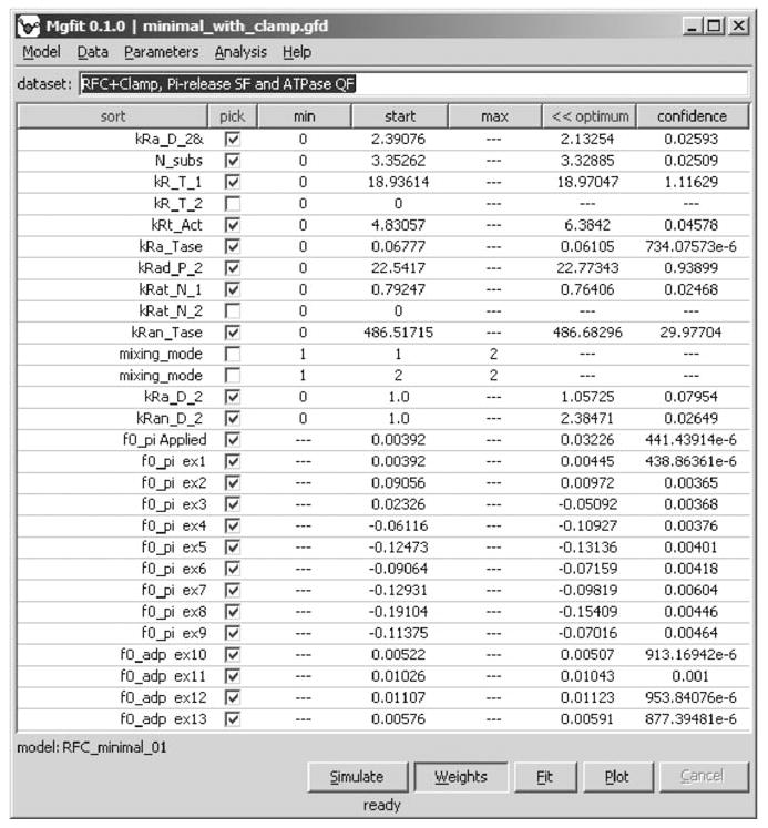
Parameters of RFC clamp loader model. The values of parameters were obtained by global fitting of 22 presteady-state kinetic measurements.

Fig. 11.

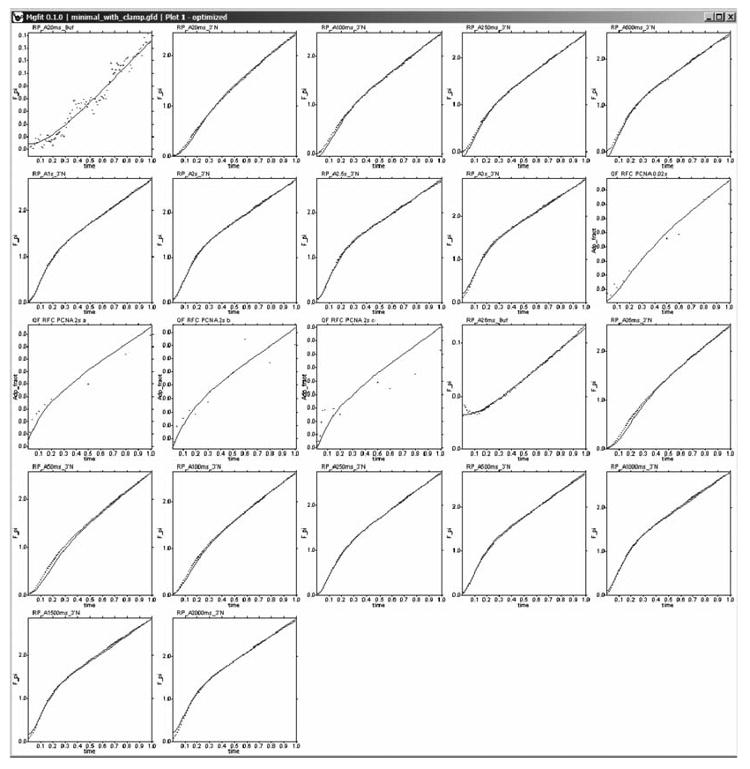
Fitting of kinetic data by the clamp loader model. Depending on the measurement conditions, kinetics of Pi release and ADP production exhibits different extent of lag followed by a burst and approach to the steady state. The presence of multiple “features” in the kinetic curves facilitates constraining parameters of the model.

Simultaneous fitting of a large number of experiments requires efficient simulation. The most computationally intensive operation performed by RFC model is integration of ODE systems to simulate mass-action reactions. To accelerate this process, reaction kinetics was simulated using native rsys library. A combination of a flexible and user-friendly scripting language, such as MATLAB, with a native library for computationally intensive parts of simulation was found to be especially productive.

Given estimates of ATP and DNA-binding rate constants, the model produces a good fit for datasets from both ATP hydrolysis as well as Pi release experiments in a single seamless operation. Confidence in the parameters obtained from the fits is increased by using the random restart method, as described in Subheading 3.2.3. A highlight of the findings is that global fitting of the ATPase data validates the proposed step between ATP binding and hydrolysis (Fig. 9C), and reveals that it is a relatively slow, and thus mechanistically important, step in the clamp assembly reaction (rate constant: kRt_Act). We can now formulate specific, testable hypotheses regarding the nature of this step; e.g., an ATP binding-driven conformational change in RFC that enables productive interactions with the clamp and DNA.

It is clear that the reaction depicted in Fig. 9C represents a simplified model of the clamp assembly reaction, in which the number of possible species and steps are restricted. Such limitations are often introduced in models to focus on specific experimentally measured parameters, and thereby increase confidence in the fit. For example, this model omits RFC binding to the clamp, since the parameters defining this step are unknown and are not measured explicitly in the ATPase experiments. Under such circumstances, however, it is entirely possible that goodness of fit to the data becomes unrelated to the quality of the model. gfit enables model-based global analysis of a variety of experiments to find parameter values that are consistent across the board. Therefore, a more comprehensive model of clamp assembly can be developed from the start, and then continually validated and refined by data input from experiments measuring clamp binding, clamp opening, DNA binding, clamp-DNA release, etc., leading to discovery of the preferred mechanism of clamp assembly on DNA.

References

- 1.Mogilner A, Wollman R, Marshall WF. Quantitative modeling in cell biology: what is it good for? Dev Cell. 2006;11:279–287. doi: 10.1016/j.devcel.2006.08.004. [DOI] [PubMed] [Google Scholar]
- 2.Albeck JG, MacBeath G, White FM, Sorger PK, Lauffenburger DA, Gaudet S. Collecting and organizing systematic sets of protein data. Nat Rev Mol Cell Biol. 2006;7:803–812. doi: 10.1038/nrm2042. [DOI] [PubMed] [Google Scholar]
- 3.Jaqaman K, Danuser G. Linking data to models: data regression. Nat Rev Mol Cell Biol. 2006;7:813–819. doi: 10.1038/nrm2030. [DOI] [PubMed] [Google Scholar]
- 4.Beechem JM. Global analysis of biochemical and biophysical data. Meth Enzymol. 1992;210:37–54. doi: 10.1016/0076-6879(92)10004-w. [DOI] [PubMed] [Google Scholar]
- 5.Draper NR, Smith H. Applied Regression Analysis. Wiley; New York: 1998. [Google Scholar]
- 6.Slepchenko BM, Schaff JC, Macara I, Loew LM. Quantitative cell biology with the Virtual Cell. Trends Cell Biol. 2003;13:570–576. doi: 10.1016/j.tcb.2003.09.002. [DOI] [PubMed] [Google Scholar]
- 7.Levin MK, Patel SS. Helicase from hepatitis C virus, energetics of DNA binding. J Biol Chem. 2002;277:29377–29385. doi: 10.1074/jbc.M112315200. [DOI] [PubMed] [Google Scholar]
- 8.Epstein IR. Cooperative and noncooperative binding of large ligands to a finite one-dimensional lattice. A model for ligand-oligonucleotide interactions. Biophys Chem. 1978;8:327–339. doi: 10.1016/0301-4622(78)80015-5. [DOI] [PubMed] [Google Scholar]
- 9.Tsodikov OV, Holbrook JA, Shkel IA, Record MT., Jr Analytic binding isotherms describing competitive interactions of a protein ligand with specific and nonspecific sites on the same DNA oligomer. Biophys J. 2001;81:1960–1969. doi: 10.1016/S0006-3495(01)75847-X. [DOI] [PMC free article] [PubMed] [Google Scholar]
- 10.Moles CG, Mendes P, Banga JR. Parameter estimation in biochemical pathways: a comparison of global optimization methods. Genome Res. 2003;13:2467–2474. doi: 10.1101/gr.1262503. [DOI] [PMC free article] [PubMed] [Google Scholar]
- 11.Banga JR. Optimization in computational systems biology. BMC Syst Biol. 2008;2:47. doi: 10.1186/1752-0509-2-47. [DOI] [PMC free article] [PubMed] [Google Scholar]
- 12.Johnson A, O Donnell M. Cellular DNA replicases: components and dynamics at the replication fork. Annu Rev Biochem. 2005;74:283–315. doi: 10.1146/annurev.biochem.73.011303.073859. [DOI] [PubMed] [Google Scholar]