Space-Time Event Sparse Penalization for Magneto-/Electroencephalography

Abstract

This article presents a new spatio-temporal method for M/EEG source reconstruction based on the assumption that only a small number of events, localized in space and/or time, are responsible for the measured signal. Each space-time event is represented using a basis function expansion which reflects the most relevant (or measurable) features of the signal. This model of neural activity leads naturally to a Bayesian likelihood function which balances the model fit to the data with the complexity of the model, where the complexity is related to the number of included events. A novel Expectation-Maximization algorithm which maximizes the likelihood function is presented. The new method is shown to be effective on several MEG simulations of neurological activity as well as data from a self-paced finger tapping experiment.

1 Introduction

The ill-posed nature of the M/EEG inverse problem is widely recognized (Baillet et al., 2001), and unique solutions are usually obtained by placing prior expectations on the nature of the brain activity associated with the measured data. In this paper we present an approach for solving the inverse problem that assumes the underlying brain activity is due to a small number or sparse set of space-time events. Each space-time event corresponds to activity that is localized spatially and in a temporal subspace. Sets of spatial and temporal basis functions are employed to represent the activity due to each space-time event and are chosen to match the characteristics of expected source activity. Seeking to explain the measured data in terms of a small number of space-time events leads to a convex optimization problem, which we solve via a novel Expectation-Maximization (EM) algorithm.

Common approaches to the M/EEG inverse problem may be classified as either parametric or imaging methods (Baillet et al., 2001). Parametric or scanning methods use a small number of dipoles (Scherg and von Cramon, 1985), multipoles (Mosher et al., 1999; Nolte and Curio, 2000), or cortical patches (Limpiti et al., 2006; Wagner et al., 2002, 2000) and scan over locations to find the best set of sources to represent the data. Examples of scanning methods include MUSIC (Mosher et al., 1992), beamforming (Van Veen et al., 1997), and maximum likelihood estimation (Dogandžić and Nehorai, 2000). One persistent challenge for scanning methods is choosing the number of sources in the solution.

The method proposed in this paper may be classified as an imaging technique. Imaging methods tessellate the brain using a large number of dipoles and attempt to simultaneously solve for all dipole amplitudes. This leads to the following linear model:

$$\mathbf{\text{Y}}=\mathbf{\text{HX}}+\mathbf{\text{N}}$$ (1)

where Y is an M × T matrix of spatio-temporal measurements from M sensors at T time points, H is an M × 3D (or M × D in the case of known dipole moment orientation) lead field matrix relating sensor measurements to D discrete dipole locations (voxels) on the cortex, X is the 3D × T signal matrix representing the unknown time courses and orientations of each dipole on the cortical surface, and N is a matrix of additive noise. The goal of imaging techniques is to estimate each element of X simultaneously given Y and H. Typically M is on the order of several hundred, while D exceeds several thousand, so Eq. (1) is severely underdetermined. Furthermore, the effective rank of H is often significantly less than M.

The problem of nonuniqueness with imaging techniques is often reduced by use of a Bayesian prior to favor some solutions over others. The prior is incorporated as a penalty term in a cost function which is minimized to estimate the neural activity. Under the assumption of white noise, these cost functions take the form:

$$\text{∑}_{t=1}^T{\Vert {\mathbf{\text{Y}}}_t-{\mathbf{\text{HX}}}_t\Vert }_2^2+{\mathrm{\lambda }}_{t}f({\mathbf{\text{X}}}_t)$$ (2)

Equation (2) is expressed in terms of individual time samples since the optimization, in most previous work, is solved separately at each time point, and solutions are often found only at specific time points selected by the user (such as signal peaks). The first term of Eq. (2) ensures that solutions explain the data well, while f acts as a penalty term. The constants λ_t balances the contribution of both terms. A common choice of penalty is simply $f({\mathbf{\text{X}}}_t)={\Vert {\mathbf{\text{WX}}}_t\Vert }_2^2$, which corresponds to a Gaussian prior on X_t, and the minimum norm estimate (MNE) is obtained with W = I. MNE has a simple closed form solution, but tends to blur activity across the cortex. The well-known LORETA technique sets W to an approximation of the Laplacian operator (Pascual-Marqui et al., 1994). Like the MNE, LORETA gives blurry, low resolution reconstructions of neuronal activity. In an effort to reduce the spatial blurring of the MNE and LORETA, the FOCUSS algorithm reinforces strong sources while deemphasizing weak ones by iteratively updating W (Gorodnitsky and Rao, 1997). FOCUSS does produce more focal estimates, but is sensitive to the initialization of W as well as to noise (Baillet et al., 2001).

Another set of methods aimed at producing focal solutions to the inverse problem use the ℓ₁ norm of X_t as a regularizer. The corresponding solutions tend to be sparse, i.e., most entries in X are zero, and can be found efficiently via linear programming. ℓ₁ penalties generally correspond to an exponential prior on X_t. Techniques differ in how to incorporate unknown dipolar orientation into the ℓ₁ penalty. The selective minimum norm (SMN) technique of Matsuura and Okabe (1995, 1997) penalizes the absolute sum of the components of each dipole. Later work by Uutela et al. (1999) uses the MNE to determine the orientation of dipolar sources, then solves the ℓ₁ penalized problem with these fixed orientations. A very recent approach for EEG called Sparse Source Imaging (SSI) replaces the ℓ₁ norm with the sum over all dipoles of the ℓ₂ norm of the three components of each dipole and solves the problem using second-order cone programming (Ding and He, 2007). In this way, SSI selects dipole orientation automatically based on the data. The criticism of ℓ₁ regularization is that it produces solutions which are “spiky” in space and inconsistent with physiological expectations. To remedy the “spiky” nature of minimum ℓ₁ solutions, another recent twist on ℓ₁ regularization in MEG, known as VESTAL, uses singular value decomposition of both the lead field matrix H and the data matrix Y (Huang et al., 2006). Here the dipole orientations are not fixed, but constrained to an octant via a diagonal sign matrix in the ℓ₁ penalty. Researchers have also proposed ℓ_p norm regularization with 0 < p < 1 and 1< p < 2 as well (Auranen et al., 2005; Jeffs et al., 1987). The optimization problem is not convex for 0 < p < 1. In general these optimization problems are more difficult to solve than p = 1, 2.

Temporal priors and sparsity have also been used to combat the ill-posed nature of the M/EEG inverse problem. Baillet and Garnero (1997) assume dipole magnitudes vary slowly with respect to sampling rate and thus penalize large changes between time samples. A similar approach is taken by Daunizeau et al. (2006) in which the second derivative of dipolar temporal evolution is penalized. Penalization of roughness encourages solutions that are low dimensional or sparse, that is, solutions implicitly described in terms of a small number of smooth bases. Dalal et al. (2008) present a parametric method for localizing cortical activity in time, frequency, and space. Localization in time and frequency implicitly assumes cortical activity is sparse in the time-frequency plane. A number of researchers have used wavelet temporal basis functions to explicitly find sparse representations of M/EEG activity. Effern et al. (2000) present a method for representing event related potentials (ERPs) recorded via EEG (or invasive cortical sensors) using a sparse set of wavelet bases. Similarly, a wavelet shrinkage procedure is used to select a small number of coefficients representing M/EEG signals prior to a Variational Bayes inversion in Trujillo-Barreto et al. (2008).

The “event sparse penalty” (ESP) regularization we present here is closely related to ℓ₁ regularization. The ESP approach seeks a solution composed of a small number of “space-time events” (STEs). Each STE is a spatio-temporal signal defined in terms of a group of basis functions. Bases are a flexible and powerful tool for balancing prior expectations of source characteristics, such as focal or bandlimited source activity, against uncertainty in exact signal behavior, such as dipole orientation or temporal evolution. The STE is constrained to lie in the space spanned by the bases, but is unconstrained within this space. Example spatial bases include x-, y-, and z- components of a dipolar source, or multipoles and patch bases for extended sources. Example temporal basis functions include Fourier bases that represent specific frequency bands, wavelets that represent desired time-frequency characteristics, and singular value decomposition (SVD) derived bases which attempt to capture temporal characteristics of the signal from the data itself.

Use of spatial and temporal bases in the ESP regularizer effectively combines the spatial and temporal aspects of the source activity estimation problem. We present ESP regularization as well as a novel Expectation-Maximization (EM) algorithm for solving the resulting optimization problem. A simple criterion for guiding the selection of an appropriate regularization parameter λ is incorporated into the optimization procedure. The effectiveness of the method is illustrated on simulations as well as human subject data from a self-paced finger tapping experiment.

The remainder of the paper is organized as follows. In Materials and Methods, we first introduce the concept of spatio-temporal basis function expansions of X in Eq. (3). This expansion allows us to define STEs and develop the ESP regularization technique for finding solutions which are sparse in STEs. Next, we present an EM algorithm for solving the ESP regularized least squares problem. The Results section describes several MEG simulations, including a set of randomized source simulations, and application of ESP regularization to MEG recordings of a subject performing self-paced finger tapping. We conclude with a discussion of the ESP method and possible extensions.

Matrices and vectors are represented by upper and lower case boldface letters, respectively. The notation e_i represents the vector of all zeros except for a one in the i^th position. Matrix inversion is represented by superscript −1, while transposition is represented by superscript T. Classic vector p norms are denoted ‖ · ‖_p, and ‖ · ‖_F denotes the Frobenius norm of a matrix. We denote the Kronecker product using the ⊗ operator while vec () concatenates columns of a matrix to produce a column vector. For a review of algebra involving ⊗ and vec (), see Brewer (1978).

2 Materials and Methods

2.1 Event Sparse Penalty Regularization

The ESP approach to the M/EEG inverse problem relies on representing the cortical signal X as a linear combination of physiologically meaningful basis functions from carefully crafted spatial and temporal dictionaries. In general, a spatio-temporal expansion of X can be written:

$$\mathbf{\text{X}}=\mathbf{\text{S}}\mathbf{\Theta }{\mathbf{\text{T}}}^T$$ (3)

where the columns of S are a dictionary containing spatial bases, the columns of T are a dictionary containing temporal bases, and the (k, l)^th element of coefficient matrix Θ specifies the contribution associated with the k^th spatial basis modulated by the l^th temporal basis. If both S and T are invertible then there is a one-to-one mapping between Θ and X, that is Θ = S⁻¹XT^−T. However, in general S and T are chosen to intentionally restrict the signal to lie in specific spatial and/or temporal subspaces in order to incorporate prior expectations into the solution of the M/EEG inverse problem, and thus are not invertible.

Given a spatio-temporal expansion in the form of Eq. (3), many methods can be used to solve the reformulated problem for Θ. In particular, regularized least squares problems analogous to Eq. (2) can be formulated with some function of Θ as the regularization term. However, improved quality solutions are possible by designing the bases and the penalty term concurrently.

Our approach assumes that M/EEG signals are the result of a small number of space-time events (STEs) which occur over limited time spans and occupy contiguous, local areas of cortex. This assumption is reflected in the following spatio-temporal expansion:

$$\begin{array}{l}\mathbf{\text{X}}=\mathbf{S}\mathbf{\Theta }{\mathbf{\text{T}}}^T=\\ \left[{\mathbf{S}}_1{\mathbf{S}}_2\dots {\mathbf{S}}_I\right]\left[\begin{array}{cccc}{\mathbf{\Theta }}_{1,1}& {\mathbf{\Theta }}_{1,2}& \dots & {\mathbf{\Theta }}_{1,J}\\ {\mathbf{\Theta }}_{2,1}& {\mathbf{\Theta }}_{2,2}& \dots & {\mathbf{\Theta }}_{2,J}\\ ⋮& ⋮& \ddots & ⋮\\ {\mathbf{\Theta }}_{I,1}& {\mathbf{\Theta }}_{I,2}& \dots & {\mathbf{\Theta }}_{I,J}\end{array}\right]\left[\begin{array}{c}{\mathbf{\text{T}}}_1^T\\ {\mathbf{\text{T}}}_2^T\\ ⋮\\ {\mathbf{\text{T}}}_J^T\end{array}\right]=\text{∑}_{i=1}^I\text{∑}_{j=1}^J{\mathbf{S}}_i{\mathbf{\Theta }}_{i,j}{\mathbf{\text{T}}}_j^T\end{array}$$ (4)

Here the spatial and temporal dictionaries, as well as the coefficient matrix, have been partitioned into space-time events. The columns of each submatrix S_i are an orthogonal basis for measurable spatial activity, such as that from a local region of cortex. Likewise, the columns of each T_j are an orthogonal basis for a temporal subspace, such as a frequency band or time interval. Cortical activity that lies in the vector space defined by a single spatial submatrix S_i and a single temporal submatrix T_j defines a single STE and is represented by the matrix of coefficients Θ_i,_j. We seek parsimonious sets of spatial and temporal bases to describe candidate STEs and formulate a criterion for finding solutions that involve a small number of non-zero Θ_i,_j.

The choice of spatial and temporal bases in Eq. (4) allows users a great deal of flexibility in both signal model and assumptions about cortical activity. The temporal bases in T_j may be chosen using wavelets, Gabor functions, Fourier bases, etc., to span time intervals and bandwidths consistent with the temporal characteristics of the signals of interest. Possible spatial bases S_i for events that activate an extended area of cortex include cortical patches (Limpiti et al., 2006; Wagner et al., 2002) and multipolar expansions (Mosher et al., 1999; Nolte and Curio, 2000). The spatial bases are also selected consistent with the spatial attributes of interest. Dipolar source bases may be used in the ESP framework.

The motivation behind Event Sparse Penalty (ESP) regularization is the assumption that the activity of interest is a collection of a small number of space-time events. This assumption, combined with appropriate spatial and temporal dictionaries, implies that the true underlying signal should have Θ_i,_j = 0 for the majority of pairs (i, j). To encourage such a sparse solution, we seek to solve an optimization problem which balances measurement error with the number of nonzero blocks Θ_i,_j. One way to do this is to penalize the least squares problem based on the number of STEs. However, this results in a nonconvex problem that requires a computationally prohibitive exhaustive search over all possible combinations of active blocks.

Many recent results have suggested that relaxing nonconvex counting functions to the convex ℓ₁ norm in regularized least squares problems provides a very good approximation to the desired regularization and results in sparse solutions (Candes and Tao, 2005; Donoho, 2006; Tropp, 2006). In the spirit of these results, we propose the ℓ₁ block penalty regularized problem:

$$\underset{\mathbf{\Theta }}{\text{min}}{\Vert \mathbf{\text{Y}}-\mathbf{\text{HS}}\mathbf{\Theta }{\mathbf{\text{T}}}^T\Vert }_F^2+\mathrm{\lambda }\text{∑}_{i,j}{\Vert \text{vec}({\mathbf{\Theta }}_{i,j})\Vert }_p$$ (5)

where p ≥ 1 is chosen to capture the magnitude of the contribution of each block. Obvious choices are p = 1, 2, or ∞. If p = 1, then the block structure of Eq. (4) is lost because the penalty in Eq. (5) becomes ‖vec (Θ) ‖₁. This encourages a solution which is sparse in the number of nonzero coefficients in Θ, but not necessarily sparse in terms of the number of STEs. If p = 2 or p = ∞, then the penalty corresponds to the ℓ₁ norm of the ℓ₂ or ℓ_∞ norm, respectively, of each block Θ_i,_j. This results in solutions that involve a small number of STEs, yet can accommodate uncertainty in the event characteristics by placing minimal restrictions on the coefficients in Θ_i,_j.

We prove in (Bolstad et al., 2007) that when one STE is present, the p = 2 case with lead field normalization (see Section 2.7) provides a higher probability of activating the correct STE than the p = ∞ case. Using p = 2 in Eq. (5) and noting that ‖vec (Θ_i,_j) ‖₂ = ‖Θ_i,_j‖_f leads to estimate Xˆ = SΘˆT^T where:

$$\widehat{\mathbf{\Theta }}=\text{arg}\underset{\mathbf{\Theta }}{\text{min}}{\Vert \mathbf{\text{Y}}-\mathbf{\text{HS}}\mathbf{\Theta }{\mathbf{\text{T}}}^T\Vert }_F^2+\mathrm{\lambda }\text{∑}_{i,j}{\Vert {\mathbf{\Theta }}_{i,j}\Vert }_F$$ (6)

This objective function is convex since it is a sum of convex functions. At least one minimizer exists since the objective function is positive (i.e., bounded below) and convex for all Θ. Section 2.3 describes a novel EM algorithm for finding Θˆ. Next we discuss possible spatio-temporal dictionary constructions.

2.2 Spatio-Temporal Dictionaries for the Inverse Problem

The ESP approach is not limited to a specific set of space-time basis functions. Degenerate choices for the basis functions in Eq. (3) transform ESP regularization into existing regularization techniques. For example, ESP can reconstruct activity independently over all time points by setting each submatrix T_j to the vector e_j, j = 1, 2,…, T. Alternatively, reconstruction at a single time point t is obtained by setting T = e_t. Degenerate choices for the spatial dictionary S combined with T = e_t results in classical ℓ₂ or ℓ₁ regularization. If S = S₁ = I and T = e_t, the estimate given by Eq. (6) at time t becomes ${\widehat{\mathbf{\Theta }}}_t=\text{arg}{\text{min}}_{{\mathbf{\Theta }}_t}{\Vert {\mathbf{\text{Y}}}_t-\mathbf{\text{H}}{\mathbf{\Theta }}_t\Vert }_2^2+\mathrm{\lambda }{\Vert {\mathbf{\Theta }}_t\Vert }_2$, which is equivalent to the MNE². Similarly, setting S = S₁ to an approximation of the surface Laplacian implements LORETA. If we assume dipole orientation is known (so that H is M × D) and use a spatial submatrix for each dipole on the cortical surface, i.e. S_i = e_i, the resulting estimate is equivalent to ℓ₁ regularization. If dipole orientation is unknown (now H is M × 3D) and S_i is chosen as a 3D × 3 matrix with a 3 × 3 identity in the position corresponding to the components of the i^th dipole in H, then ESP corresponds to the recently proposed SSI formulation of the EEG inverse problem (Ding and He, 2007) ³. In this case ESP encourages a solution with a small number of dipoles while identifying the unknown dipole orientations.

The power of the ESP approach is that it allows for more general and flexible spatial and temporal representations of expected source activity than these degenerate examples. Temporal bases can be used, for example, to isolate a desired frequency band, or may be grouped into different frequency bands such that, for example, T₁ spans the α-band, T₂ the β-band, T₃ the γ-band and so on, reflecting the expectation that different source activity occupies different bands. Temporal bases can also be used to isolate time ranges. Alternatively wavelets or other time-frequency bases can be used to identify source activity based on time-frequency characteristics analogous to Dalal et al. (2008). Similarly, the spatial bases can represent spatially extended source activity The expectation that signals occupy extended areas rather than single dipoles is discussed, for example, in (Baillet and Garnero, 1997; Daunizeau and Friston, 2007). Representations for multipoles and cortical patches have been proposed to accommodate extended source activity (Limpiti et al., 2006; Mosher et al., 1999; Wagner et al., 2002, 2000) and are easily incorporated as bases, as we illustrate in Section 3.

2.3 Expectation-Maximization Algorithm

The gradient of Σ_i,_j‖Θ_i,_j‖₂ is discontinuous so classical gradient-based minimization approaches to Eq. (6) can not be used without modification. Instead, we have developed an Expectation-Maximization (EM) algorithm which treats the objective of Eq. (6) as a negated Bayesian log-likelihood function where the penalty can be interpreted as the logarithm of a prior distribution on Θ. EM finds the maximum a posteriori (MAP) estimate of Θ. The approach described here is a generalization of the EM algorithm developed by Figueiredo and Nowak (2003). The pioneering work on EM was published by Dempster, Laird, and Rubin (Dempster et al., 1977).

The EM algorithm monotonically increases the Bayesian likelihood p(Y∣Θ)p(Θ) over Θ. Assuming white Gaussian noise and the density $p(\mathbf{\Theta })\propto \text{exp}\left\{-\frac{\mathrm{\lambda }}{2{\sigma }^2}{\sum }_{i,j}{\Vert {\mathbf{\Theta }}_{i,j}\Vert }_F\right\}$, the negated Bayesian log-likelihood is proportional to $\frac{{\Vert \mathbf{\text{Y}}-\mathbf{\text{HS}}\mathbf{\Theta }{\mathbf{\text{T}}}^T\Vert }_F^2}{2{\sigma }^2}+\frac{\mathrm{\lambda }}{2{\sigma }^2}{\sum }_{i,j}{\Vert {\mathbf{\Theta }}_{i,j}\Vert }_F$. Multiplying through by 2σ², we see that the EM algorithm is monotonically decreasing the function ${\Vert \mathbf{\text{Y}}-\mathbf{\text{HS}}\mathbf{\Theta }{\mathbf{\text{T}}}^T\Vert }_F^2+\mathrm{\lambda }{\sum }_{i,j}{\Vert {\mathbf{\Theta }}_{i,j}\Vert }_F$, which is the objective of Eq. (6).

The key aspect of solving an estimation problem via the EM algorithm is to identify a so-called “hidden data set” which, if known, would make the problem easy to solve. EM alternates between solving the easy problem given an estimate of the hidden data and updating the estimate of the hidden data. We identify hidden data Z for the ESP problem based on the decomposition:

$$\mathbf{Z}=\mathbf{\Theta }+\alpha {\mathbf{N}}_1$$ (7)

$$\mathbf{Y}=\mathbf{\text{HSZ}}{\mathbf{T}}^T+{\mathbf{N}}_2$$ (8)

Here the noise matrix N of Eq. (1) is decomposed into two independent random matrices N₁ and N₂ with distributions vec (N₁) ∼ N(0, I ⊗ I) and vec (N₂) ∼ N(0, σ²I − α²TT^T ⊗ HSS^TH^T). The scalar α² must satisfy α² < σ²‖TT^T‖⁻¹‖HSS^TH^T‖⁻¹ so that a valid covariance matrix exists for N₂. With this decomposition, estimating Θ given Z amounts to a classic denoising problem (Donoho, 1995) in which the density of the desired signal Θ is characterized by the penalty function Σ_i,_j ‖Θ_i,_j‖_F. Equation (8) is then used to update the estimate of Z.

The EM algorithm alternates between an Expectation Step (E-Step) and a Maximization Step (M-Step). The E-Step calculates the Q-function: Q(Θ∣Θˆ^(k−1)) ≡ E[log p(Y, Z∣Θ)∣Y,Θˆ^(k−1))] where the expectation is over Z and Θˆ^(k−1) is the estimate from the previous iteration. The M-Step maximizes Q(Θ∣Θˆ^(k−1))+ log p(Θ) over Θ to produce Θˆ^{(k) 4}. This produces a series of iterates Θˆ^(k) which are guaranteed to converge to a stationary point provided that Q(A∣B) is continuous in both A and B (Wu, 1983).

In the E-Step, we calculate the Q-function using the measured data and the estimate Θˆ^(k−1):

$$\begin{array}{cc}Q(\mathbf{\Theta }|{\widehat{\mathbf{\Theta }}}^{(k-1)})& =E[\text{log}p\left(\mathbf{\text{Y}},\mathbf{\text{Z}}|\mathbf{\Theta }\right)|\mathbf{\text{Y}},{\widehat{\mathbf{\Theta }}}^{(k-1)})]\hfill \\ & =K-\frac{{\Vert \mathbf{\Theta }-{\widehat{\mathbf{\text{Z}}}}^{(k)}\Vert }_F^2}{2{\alpha }^2}\hfill \end{array}$$ (9)

where K is not a function of Θ and:

$$\begin{array}{cc}{\widehat{\mathbf{\text{Z}}}}^{(k)}& =E[\mathbf{\text{Z}}|\mathbf{\text{Y}},{\widehat{\mathbf{\Theta }}}^{(k-1)}]\hfill \\ \hfill & ={\widehat{\mathbf{\Theta }}}^{(k-1)}+\frac{{\alpha }^2}{{\sigma }^2}{\mathbf{\text{S}}}^T{\mathbf{\text{H}}}^T(\mathbf{\text{Y}}-\mathbf{\text{HS}}{\widehat{\mathbf{\Theta }}}^{(k-1)}{\mathbf{\text{T}}}^T)\mathbf{\text{T}}\end{array}$$ (10)

Thus, specifying Q(Θ∣Θˆ^(k−1)) amounts to calculating Zˆ^(k) using Eq. (10).

The M-Step is a generalization of the M-Step for an ℓ₁ penalized least squares problem (see Figueiredo and Nowak (2003)) since the penalty in Eq. (6) is a generalization of the ℓ₁ norm. We seek to solve the following problem:

$$\begin{array}{cc}{\widehat{\mathbf{\Theta }}}^{(k)}& =\text{arg}\underset{\mathbf{\Theta }}{max}Q(\mathbf{\Theta }|{\widehat{\mathbf{\Theta }}}^{(k-1)})+logp\left(\mathbf{\Theta }\right)\hfill \\ & =\text{arg}\underset{\mathbf{\Theta }}{\text{min}}\left\{\frac{{\Vert \mathbf{\Theta }-{\widehat{\mathbf{\text{Z}}}}^{(k)}\Vert }_F^2}{2{\alpha }^2}+\frac{\mathrm{\lambda }}{2{\sigma }^2}\text{∑}_{i,j}{\Vert {\mathbf{\Theta }}_{i,j}\Vert }_F\right\}\end{array}$$ (11)

This is the maximum a posteriori estimate of Θ given Zˆ^(k) assuming $p(\mathbf{\Theta })\propto exp\left(-\frac{\mathrm{\lambda }}{2{\sigma }^2}{\sum }_{i,j}{\Vert {\mathbf{\Theta }}_{i,j}\Vert }_F\right)$. The key feature facilitating the solution of Eq. (11) is the separability of the problem into blocks corresponding to the blocks of Eq. (4):

$$\frac{{\Vert \mathbf{\Theta }-{\widehat{\mathbf{\text{Z}}}}^{(k)}\Vert }_F^2}{2{\alpha }^2}+\frac{\mathrm{\lambda }}{2{\sigma }^2}\text{∑}_{i,j}{\Vert {\mathbf{\Theta }}_{i,j}\Vert }_F=\text{∑}_{i,j}\frac{{\Vert {\mathbf{\Theta }}_{i,j}-{\widehat{\mathbf{\text{Z}}}}_{i,j}^{(k)}\Vert }_F^2}{2{\alpha }^2}+\frac{\mathrm{\lambda }}{2{\sigma }^2}{\Vert {\mathbf{\Theta }}_{i,j}\Vert }_F$$ (12)

We solve Eq. (11) by finding the Θ_i,j that minimizes ${\Vert {\mathbf{\Theta }}_{i,j}-{\widehat{\mathbf{\text{Z}}}}_{i,j}^{(k)}\Vert }_F^2+\frac{{\alpha }^2\mathrm{\lambda }}{{\sigma }^2}{\Vert {\mathbf{\Theta }}_{i,j}\Vert }_F$ for every pair (i, j). The single block problem for the (i, j)^th block is rewritten in simplified notation using $\mathbf{\text{z}}=\text{vec}\left({\widehat{\mathbf{\text{Z}}}}_{i,j}^{(k)}\right)$ and θ = vec (Θ_i,j) as $f(\theta )={\Vert \theta -\mathbf{\text{z}}\Vert }_2^2+\frac{{\alpha }^2\mathrm{\lambda }}{{\sigma }^2}{\Vert \theta \Vert }_2$. Since f(θ) is strictly convex, it has a unique minimizer θ*. We show in Appendix A that:

$${\theta }^{\ast }=\{\begin{array}{cc}(1-\frac{{\alpha }^2\mathrm{\lambda }}{2{\sigma }^2{\Vert \mathbf{\text{z}}\Vert }_2})\mathbf{\text{z}},& \text{if}{\Vert \mathbf{\text{z}}\Vert }_2>\frac{{\alpha }^2\mathrm{\lambda }}{2{\sigma }^2}\\ 0,\hfill & \text{otherwise}\end{array}$$ (13)

We summarize the k^th iteration of the EM algorithm as:

$$\begin{array}{l}{\widehat{\mathbf{\text{Z}}}}^{(k)}={\widehat{\mathbf{\Theta }}}^{(k-1)}+c{\mathbf{\text{S}}}^T{\mathbf{\text{H}}}^T(\mathbf{\text{Y}}-\mathbf{\text{HS}}{\widehat{\mathbf{\Theta }}}^{(k-1)}{\mathbf{\text{T}}}^T)\mathbf{\text{T}}\\ {\widehat{\mathbf{\Theta }}}^{(k)}=\text{arg}\underset{\mathbf{\Theta }}{\text{min}}\left\{{\Vert \mathbf{\Theta }-{\widehat{\mathbf{\text{Z}}}}^{(k)}\Vert }_F^2+c\mathrm{\lambda }\text{∑}_{i,j}{\Vert {\mathbf{\Theta }}_{i,j}\Vert }_F\right\}\end{array}$$ (14)

where c acts as a step size parameter. Setting α² at the upper bound α² = σ²‖TT^T‖⁻¹‖HSS^TH^T‖⁻¹ leads to c = ‖TT^T‖⁻¹‖HSS^TH^T‖⁻¹. This step size guarantees a decrease in the objective function at each iteration; however, following recent work by Wright et al. (2008), we add an inner loop to the algorithm which starts with a larger step size, then reduces c until the objective function decreases. This simple modification speeds up convergence of the algorithm by one to two orders of magnitude.

As described in (Wu, 1983), continuity of the Q function and the existence of a lower bound to Eq. (6) implies convergence to a stationary point. Since Eq. (6) is convex, the only stationary points are global minima, and Θˆ^(k) converges to a global minimizer. Various stopping criteria may be used to terminate the algorithm. To ensure a correct solution has been reached, we run the algorithm until the subgradient condition (i.e., the subdifferential of Eq. (6) at Θˆ contains 0) is satisified to within a small tolerance.

2.4 EM Continuation

An advantage of our EM algorithm approach is that it provides an easy means to calculate solutions Θˆ(λ) for a wide variety of λ via a “continuation” approach. Since a small change in λ does not typically produce a large change in Θˆ (λ), the solution Θˆ (λ₁) can be used to initialize the algorithm when solving for Θˆ(λ₂). If λ₂ ≈ λ₁, then this initialization point will be close to Θˆ(λ₂). Furthermore, we show in Appendix B that Θˆ(λ) = 0 for λ ≥ λ_MAX, where:

$${\mathrm{\lambda }}_{\mathit{\text{MAX}}}=2{\Vert \underset{i,j}{\text{max}}{\mathbf{\text{S}}}_i^T{\mathbf{\text{H}}}^T{\mathbf{\text{YT}}}_j\Vert }_2$$ (15)

depends on the data Y. Thus, we solve for a range of λ by setting Θˆ(λ_MAX) = 0, and then solving for λ = (1 − ε)λ_MAX using 0 as the initial guess with ε small, e.g. 0.01. Next we use Θˆ((1 − ε)λ_MAX) as a starting point to find Θˆ((1 − 2ε)λ_MAX) and continue in this manner until we arrive at the desired λ. Selection of λ is discussed in Section 2.6.

2.5 EM Algorithm Performance

The EM algorithm described above solves Eq. (6) efficiently compared to second-order cone programming (SOCP) methods often used to minimize cost functions similar to Eq. (6) (e.g., Ding and He (2007); Malioutov et al. (2005); Ou et al. (2009)). The most computationally expensive calculation in EM is matrix multiplication, namely (HS)Θˆ^(k−1)T^T and (HS)^TRT (where R = Y − HSΘˆ^(k−1)T^T). This requires O((K + T)ML) operations (note that significantly fewer operations are typically required since Θˆ^(k−1) is mostly zeros). In contrast SOCP methods require O(((M + K)L)³) operations per iteration when a single temporal block is used, i.e. T = T₁ (Ou et al., 2009). The cubic complexity of SOCP can be prohibitive in large problems.

There are also qualitative differences between solutions found by EM and those found by SOCP. Solutions found by SOCP are not sparse; that is, many of the coefficients are very small, but not zero. This means users must define some threshold to decide which blocks of coefficients should be set to zero. In contrast EM returns truly sparse solutions, with most Θˆ_i,j = 0, eliminating the threshold selection problem. The fact that most Θˆ_i,j = 0 follows from the M-Step shrinkage procedure (see Eq. (13)). It is known that exact solutions to ℓ₁ penalized regularization problems are truly sparse (see e.g. Donoho (2006)). Also note that our EM approach efficiently finds solutions for multiple λ, while SOCP must start from scratch for each λ of interest.

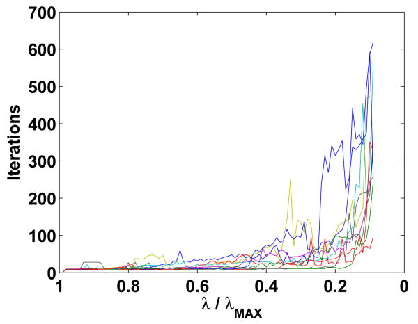
The main criticism of EM algorithms in general is that they converge slowly when the cost function is relatively flat. This slow convergence is resolved in three ways in the ESP procedure. First, our modified EM algorithm uses a variable step size to speed up convergence in flat areas (see Sec. 2.3). Second, EM typically identifies nonzero Θˆ_i,j quickly, but takes longer to adjust the coefficients within in each block. Since debiasing is typically applied to the EM result (see Sec. 2.8), the algorithm may be stopped once the “sparsity pattern” has stabilized. Third, use of EM continuation (see Sec. 2.4) provides a sequence of good initial guesses. Examples of convergence behavior are given in Fig. (15).

Fig. 15.

Number of EM algorithm iterations required for each λ for all ten trials of Example 2 (Table 1). Solutions are calculated beginning with λ = λ_MAX as described in Sec. 2.4.

2.6 Penalty Weight Parameter Selection

The quality of the estimate Θˆ given by Eq. (6) depends on the penalty weight parameter λ. Intuitively, large λ corresponds to heavy reliance on the prior and gives a very sparse (or all zero) estimate, while small λ corresponds to heavy reliance on the noisy data and gives solutions with activity spread all over the cortical surface. Clearly, both of these extremes are undesirable. In general, user expertise may provide the best results for selecting λ, and in many cases it may be desirable to consider a range of solutions from multiple values of λ. However, automatic selection of λ is necessary for objective performance evaluation and to provide a starting point for user based selection.

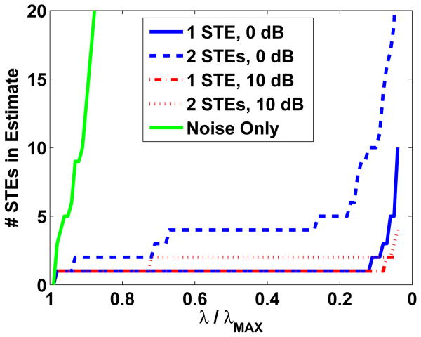
We have developed a simple heuristic to automate selection of λ based on the number of nonzero Θ_i,j, that is, the cardinality of Aˆ(λ) = {(i, j)∣Θˆ_i,j(λ) ≠ 0}. The intuition behind our heuristic is the following. Suppose no signal is present, i.e. Y = N, and we solve Eq. (6). Since white noise is spread roughly equally through all subspaces, no single block Θ_i,j can account for a significant portion of the measured data Y. Thus, as λ decreases, the number of blocks in Aˆ(λ) increases rapidly to reduce the error term in Eq. (6). In contrast, when a signal described by a small number of STEs is present, the signal portion of the measured data can be explained by the corresponding blocks, and initially the cardinality of Aˆ(λ) increases relatively slowly as λ decreases. Once the active blocks are able to explain the signal component of the data, then additional blocks attempt to represent noise and the number of active blocks will increase rapidly as λ is decreased further. This behavior is illustrated in Fig. 1. Note that the number of STEs increases rapidly as λ decreases for the noise only case, while it initially increases very slowly when signal components are present.

Fig. 1.

Characteristic behavior of the number of STEs identified by ESP vs. λ/λ_MAX. The presence of source activity results in a plateau in the number of STEs selected as λ/λ_MAX decreases.

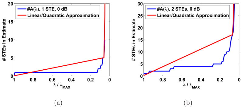
These observations suggest a simple strategy analogous to the L-curve method of regularization in which we select the value of λ where the number of STEs begins to increase rapidly with further decrease in λ. We implement one such strategy by comparing the cardinality of Aˆ(λ), which we denote #A(λ), with a piecewise approximation based on two curve segments: a linear function for large λ and quadratic function for small λ. The linear function connects the points (λ_MAX, 0) and (λ, #A(λ)). The quadratic function is uniquely defined by two fixed endpoints since it is purely quadratic (i.e., has no linear term). The endpoints used for the quadratic are (λ, #A(λ)) and (0, #Aˆ(0)), where #Aˆ(0) is a rough estimate of #A(0) found by dividing the rank of the forward model by the number of bases in each block. This is the number of active blocks required to produce an estimate which fits any measured data exactly We vary λ to find the value that minimizes the squared error between #A(λ) and the piecewise approximation. This value of λ is used to identify the approximate point at which the transition between fitting signal and noise occurs.

This method of λ selection requires that #A(λ) be calculated for small enough λ such that the characteristic shape of Fig. 1 is observed before applying the heuristic. Two examples of the heuristic λ selection are shown in Fig. 2. These two examples suggest that the λ selected with this heuristic is typically smaller than the “optimal” λ. Hence, this heuristic provides a good lower bound on λ.

Fig. 2.

Example of heuristic applied to 0 dB simulated data with (a) 1 STE and (b) 2 STEs.

2.7 Non-white Noise and Lead Field Normalization

A key assumption behind the ESP method as presented so far is that the signal is contaminated with white noise. We accommodate colored noise by first whitening the data with the noise covariance matrix. Suppose the noise in Eq. (1) is distributed N ∼ N(0, R_N). Taking the matrix square root ${\mathbf{\text{R}}}_N={\mathbf{\text{R}}}_N^{1/2}{\mathbf{\text{R}}}_N^{T/2}$, the whitened data is:

$$\stackrel{\sim }{\mathbf{\text{Y}}}={\mathbf{\text{R}}}_N^{-1/2}\mathbf{\text{Y}}={\mathbf{\text{R}}}_N^{-1/2}\mathbf{\text{HX}}+{\mathbf{\text{R}}}_N^{-1/2}\mathbf{\text{N}}=\stackrel{\sim }{\mathbf{\text{H}}}\mathbf{\text{X}}+\stackrel{\sim }{\mathbf{\text{N}}}$$ (16)

where N˜ ∼ N(0, I). ESP is applied to the whitened system. In practice R_N is usually unknown, so whitening requires that R_N be estimated from available data.

After whitening the data and expanding the signal with ESP basis functions, the signal model is:

$$\stackrel{\sim }{\mathbf{\text{Y}}}=\stackrel{\sim }{\mathbf{\text{H}}}\mathbf{\text{S}}\mathbf{\Theta }{\mathbf{\text{T}}}^T+\stackrel{\sim }{\mathbf{\text{N}}}$$ (17)

We normalize the lead fields using diagonal matrix W whose entries equal the ℓ₂ norm of the corresponding column of H˜S. This eliminates bias toward sources that are closest to the sensors. Thus we have:

$$\stackrel{\sim }{\mathbf{\text{Y}}}=\stackrel{\sim }{\mathbf{\text{H}}}{\mathbf{\text{SW}}}^{-1}\mathbf{\text{W}}\mathbf{\Theta }{\mathbf{\text{T}}}^T+\stackrel{\sim }{\mathbf{\text{N}}}$$ (18)

Here the columns of the matrix H˜SW⁻¹ are unit norm due to the normalization. The columns of T may be normalized as well, though typically the T_j are constructed so that ${\mathbf{\text{T}}}_j^T{\mathbf{\text{T}}}_j=\mathbf{\text{I}}$ and thus normalization of T is not necessary. The EM algorithm solves for Θ′ = WΘ.

2.8 Debiasing

The penalty in Eq. (6) tends to “shrink” the coefficient matrices Θ_i,j and produces biased amplitude estimates. This bias can be removed by using ESP to estimate the set of active STEs: A = {(i, j)∣Θ_i,j ≠ 0} and then solving a least squares problem on this set to produce a refined estimate of Θ_i,j, for all (i, j) ∈ A. We employ a minimum norm solution to the inverse problem defined on active blocks A to obtain the refined estimate. This process is referred to as debiasing in (x02113)₁ regularized inverse problems since it removes some of the bias introduced by the penalty term in Eq. (6). Note that debiasing does not alter the spatial or temporal extent of the ESP solution e.g., introduce blurring, since the set of active STEs does not change. The debiasing step may be performed without lead field normalization. Also, different basis expansions for the active blocks may be used in debiasing than those used for the original ESP regularization. The debiasing step is not necessary for the ESP regularization approach, especially if source localization is the primary goal.

3 Results

We illustrate examples of ESP reconstruction in this section. We begin by describing the specific spatio-temporal bases used for the examples. Next, we present a simulation in which the true activity consists of three space-time events and the measurements are contaminated by realistic sensor noise, followed by results from a randomized simulation involving two cortical signals. Finally, we apply ESP reconstruction to measurements collected during a self-paced finger tapping experiment.

3.1 Space- Time Basis Function Selection for Examples

As noted previously there are many possible ways to define STEs. We illustrate the attributes of the ESP reconstruction approach using STEs defined spatially by cortical patches and temporally by fixed time windows and a common bandwidth. Use of cortical patches to design spatial bases results in event bases that are locally supported and particularly parsimonious. This significantly reduces the dimension of the inverse problem. The basis construction procedure described here exemplifies several key attributes of appropriate bases and is derived from the cortical patch bases of Limpiti et al. (2006).

Assume the i^th cortical patch is tessellated with a set of dipoles whose lead fields and amplitudes are concatenated into a patch lead field matrix Hⁱ and amplitude vector αⁱ, respectively. Hence, the signal yⁱ measured at the sensors due to the i^th patch is yⁱ = Hⁱαⁱ. The bases representing events in this patch should only describe the space of possible activity distributions αⁱ that contribute to the measurement. To this end, take the singular value decomposition of Hⁱ = UⁱΣⁱV^iT where the columns of Uⁱ and Vⁱ are the left and right singular vectors, respectively, and Σⁱ is a diagonal matrix of singular values ordered from largest to smallest. Typically Hⁱ is low rank (Limpiti et al., 2006) so a small number of the singular values are significant.

The columns of Vⁱ are a natural basis for the patch signal αⁱ. Hence, we may express ${\alpha }^i={\sum }_k{a}_k{\mathbf{\text{v}}}_k^i$ where ${\mathbf{\text{v}}}_k^i$ is the k^th column of Vⁱ and a_k are the expansion coefficients. The corresponding signal measured at the sensor is:

$${\text{Y}}^i=\text{∑}_k{a}_k{\mathbf{\text{u}}}_k^i{\sigma }_k^i$$ (19)

where ${\mathbf{\text{u}}}_k^i$ is the k^th column of Uⁱ and ${\sigma }_k^i$ is the k^th largest singular value. The strength of the k^th component of the measured signal is proportional to ${\sigma }_k^i$, so spatial bases ${\mathbf{\text{v}}}_k^i$ associated with small singular values make small contributions to the measured signal. Given the typically low signal to noise ratio of M/EEG, the measurable spatial component of an STE from the i^th patch is adequately represented by the right singular vectors corresponding to the largest singular values. Hence, we construct the spatial basis S_i from the “significant” right singular vectors associated with the i^th patch.

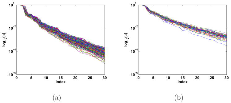
Figure 3 depicts the singular values for two sets of patches computed for the 275 channel CTF MEG system. The singular values shown in Figure 3(a) correspond to all 393 patches of geodesic radius 20 mm which tile both hemispheres of a subject with 50% overlap. Note that in each case the 7^th and higher singular values are an order of magnitude smaller than the largest singular value. Furthermore, the first two or three singular values are five times larger than the higher order singular values. The number of significant singular values is related to the size of the patch. Figure 3(b) shows singular values corresponding to 57 patches of geodesic radius 50 mm which again tile both hemispheres with 50% overlap. The singular values for the larger patches decay more slowly; the 10^th and higher singular values are an order of magnitude smaller than the largest singular value in a given patch.

Fig. 3.

Normalized singular values associated with patch lead field matrices from (a) 393 patches of 20 mm geodesic radius and (b) 57 patches of 50 mm geodesic radius which span the cortical surface with 50% overlap. The singular values decay rapidly in every patch.

Figure 4 illustrates the spatial pattern associated with several right singular vectors for a typical 20 mm patch by depicting each element of v_k at the corresponding dipole location in the patch. The singular vectors associated with the largest singular values tend to represent low resolution features within the patch. The level of detail or fine structure represented by a singular vector increases as the corresponding singular values decrease. Selecting the number of significant singular values and vectors thus involves a tradeoff between representing the details of the spatial distribution of activity within the patch and having adequate SNR to estimate the detail. Relatively high SNR is required to reliably identify the fine structure associated with small singular values. Similar tradeoffs exist with other approaches to choosing spatial bases. For example, the contributions of higher order terms in a multipole expansion also decay rapidly, so the SNR dictates the number of terms that can be reliably estimated and used as spatial bases.

Fig. 4.

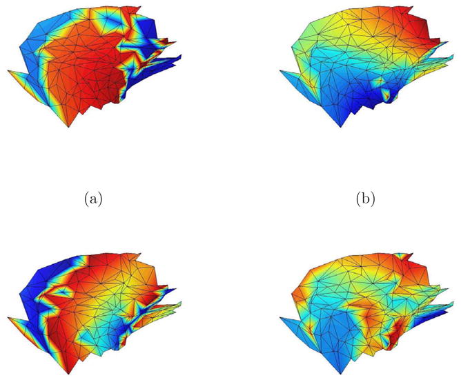
Color cortical activity pattern for singular vectors v_k of a representative patch. The vertices in the mesh represent dipole locations in the cortical tessellation of the patch. (a) v₁, largest singular value. (b) v₃, third largest singular value. (c) v₅, fifth largest singular value. (d) v₇, seventh largest singular value. The activity patterns associated with larger singular values tend to represent low resolution features within the patch, while those associated with smaller singular values represent fine structure.

For the examples that follow, we choose patches of 20 mm geodesic radius on the cortical surface extracted from an MRI of the subject. Note that geodesic distances calculated using the edges of triangles representing the cortical surface are greater than the true geodesic distance. Figures 13 and 14 illustrate typical 20 mm patches. We choose three spatial bases per patch for each STE since the majority of measurable activity in any patch is represented by the first three singular vectors, as indicated in Fig. 3.

Fig. 13.

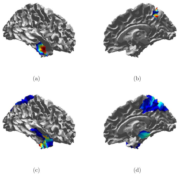
True signal and debiased ESP reconstruction of Trial 6 from Table 1. (a) Source 1 spatial extent. (b) Source 2 spatial extent. (c) Debiased ESP reconstruction of source 1 at 41 ms. (e) Debiased ESP reconstruction of source 2 at 55 ms.

Fig. 14.

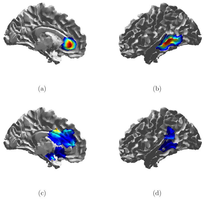
True signal and debiased ESP reconstruction of Trial 8 from Table 1. (a) Source 1 spatial extent. (b) Source 2 spatial extent. (c) Debiased ESP reconstruction of source 1 at 66 ms. (e) Debiased ESP reconstruction of source 2 at 37 ms.

We represent the temporal aspect of STEs for our examples by dividing the total time extent of interest into time windows that overlap by 50%. A wavelet basis that spans the frequency band of interest (0-100 Hz) is used for each window. We have found that wavelet bases result in smooth transitions at the window edges. We use 32 wavelets per time interval, so the number of coefficients associated with each STE is 96 (Θ_i,j is 3 by 32).

3.2 Simulated Example 1

We test the ESP approach using simulated data from a 275 channel CTF MEG system. The simulated cortical signal consists of three STEs: activation of a patch in both the left and right primary auditory cortex with a slight offset in time followed by a patch of activity in the motor cortex. All three simulated patches have geodesic radii of roughly 10 mm. The patches used as simulated sources do not correspond to patches used in the ESP procedure; the simulated source patches are smaller and have different center locations. Furthermore, the simulated spatial activity pattern within each patch (raised cosine) does not correspond to the singular vectors used to represent any patch. Lastly, the temporal evolution of the signal, although primarily low-pass, does not correspond directly to the wavelet bases used in reconstruction. The measurements are simulated using Eq. (1) for 60 trials, with N consisting of spatially colored noise drawn from a N(0, I⊗R) distribution where R was calculated from the prestimulus portion of an MEG experiment. The noise level is set to achieve an average SNR (defined as ${\Vert \mathbf{\text{HX}}\Vert }_F^2/E[{\Vert \mathbf{\text{N}}\Vert }_F^2]$) of -6 dB after averaging over all epochs. Figure 5 illustrates the time courses and spatial extents of the three space-time events, as well as the noisy measurements.

Fig. 5.

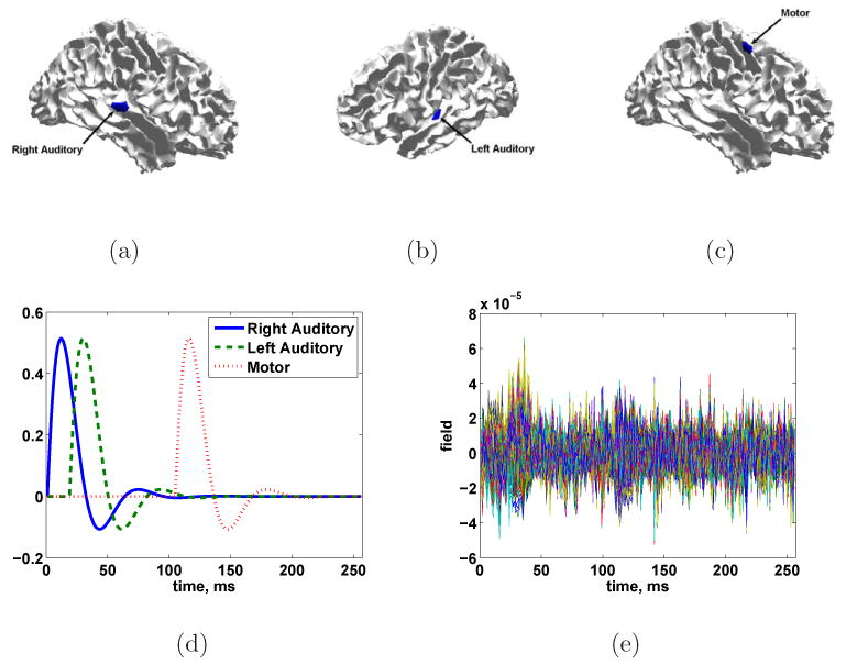
Simulated three source scenario. True source location and spatial extent of sources at times (a) 12, (b) 30, and (c) 116 ms. (d) True source time courses. (e) Simulated signals in noise for SNR = -6 dB.

After whitening the data as described in Section 2.7 using a noise covariance matrix estimated by removing the mean from each trial, we apply ESP reconstruction to the simulated signal using the STEs described in Section 3.1. We use 7 overlapping time windows of 64 ms each. Combined with the 393 spatial patches, this results in a total of 2751 candidate STEs, each with 96 coefficients.

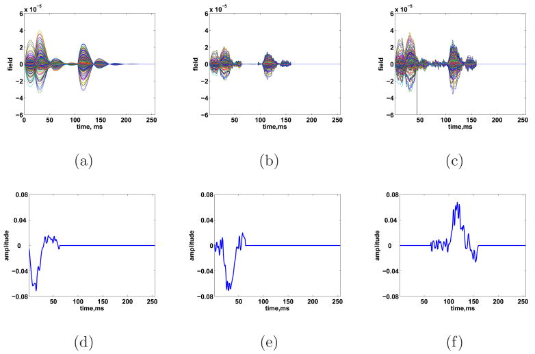
The heuristic of Section 2.6 is used to select λ. The result of debiasing the ESP reconstruction for this λ is shown in Figs. 6 and 7. All three STEs are recovered at the correct locations in space and time. Activity is spread spatially around the true location. Some of this spreading is due to the use of larger patches in the ESP reconstruction, while some spreading is inherent to the ill-posed nature of the inverse problem. We also point out that some temporal spreading occurs as a result of noise lying in the subspace defined by fixed time windows.

Fig. 6.

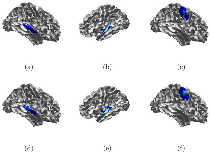
Cortical signal estimate from ESP before (a – c) and after (d – f) debiasing. Estimates shown for peak signal times: (a,d) 12 ms, (b,e) 30 ms, and (c,f) 116 ms.

Fig. 7.

(a) Noise free simulated data (b) ESP reconstruction of sensor measurements before debiasing (c) ESP reconstruction of sensor measurements after debiasing. Estimated temporal evolution of: (d) a single dipole in the right auditory cortex, (e) a single dipole in the left auditory cortex, and (f) a single dipole in the left motor cortex.

This is evident between 97 and 105 ms, where the motor cortex exhibits low-level activity in the reconstruction, though the true motor activity starts at 106 ms. The fixed time window in which the motor cortex is active begins at 97 ms. The reconstructed cortical activity in Fig. 7(d) – 7(f) is consistent with the true sources depicted in Fig. 5(d).

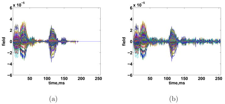
We now illustrate the flexibility of ESP by employing different sets of temporal basis functions for the T_j. We also show the advantage of assuming sparsity in the temporal domain. First, we use the same seven overlapping time windows, but perform singular value decomposition (SVD) of the noisy data in each window and keep the two most significant singular vectors for each T_i – at most two singular values are visibly much larger than the others in the SVDs of the data in each window. The technique of using SVD of the data to determine the temporal signal subspace has been used previously in M/EEG (Huang et al., 2006; Ou et al., 2009). The resulting reconstruction after heuristic λ selection 8(a). The result is similar to that obtained using wavelet bases, although there is some additional spatial blurring (not shown). Next, we repeat the experiment with temporal bases derived from the SVD of the entire time period of the experiment (e.g. 0 to 256 ms). We use the three most significant singular vectors to form T = T₁. The result after heuristic λ selection and debiasing is shown in Figs. 8(b) and 9. In this case, the reconstructed activity extends throughout the measurement period due to the influence of noise on the SVD bases, even though the true signal becomes negligible after about 200 ms. Also, Fig. 9 shows that each cortical area involved in the signal estimate has activity which persists throughout the measurement period. This example shows the advantage of assuming sparsity in the temporal domain; when time windows are used, ESP can automatically set the estimate Xˆ_t to zero when there is not sufficient evidence of activity during a particular time period, and identify the time intervals when each source is active.

Fig. 8.

(a) Reconstructed sensor measurements using multiple time windows and SVD temporal basis functions. (b) Reconstructed sensor measurements using single time window and SVD temporal basis functions.

Fig. 9.

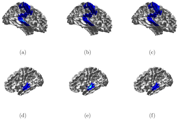
Reconstructed cortical signal using a single temporal block at time: (a,d) 12 ms (b,e) 30 ms (c,f) 116 ms.

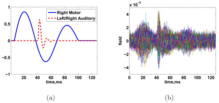
In our final variation on this example, we illustrate an alternative way to exploit sparsity in the temporal domain. Here we consider a scenario involving a “slow” event which spans a long period of time and two “fast” events spanning much shorter time periods. These signals are illustrated in Fig. 10. Simulated measurements are generated using Eq. (1) assuming white noise at 0 dB. We apply ESP using multiscale temporal blocks. For T₁ we use 32 low frequency, large scale wavelets which occupy the entire time period. In contrast, T₂ and T₃ consist of 32 wavelets each spanning, respectively, the first and second half of the 256 ms measurement period. Thus the temporal blocks implement a time-frequency partition of the data. We illustrate the resulting reconstruction (after heuristic λ selection and debiasing) in Fig. 11. ESP estimates the “slow” portion of the data using the large scale wavelets (T₁). The “fast” components are reconstructed with the shorter scale, higher frequency bases of T₂. T₃ is identified by ESP as inactive. This example illustrates the use of temporal sparsity to identify events spanning different time scales. Similarly, by appropriate basis selection, temporal sparsity can be used to identify events spanning different frequency bands.

Fig. 10.

(a) Temporal evolution of true activity. (b) Simulated noisy sensor measurements.

Fig. 11.

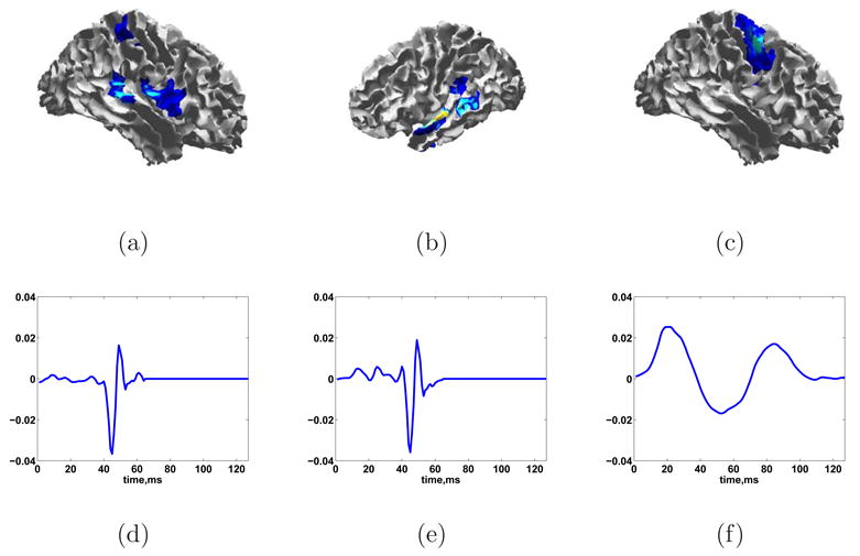
Reconstructed cortical signal using temporal bases spanning multiple scales. Cortical activation and temporal evolution in the: (a,d) right auditory cortex, (b,e) left auditory cortex, and (c,f) right motor cortex.

3.3 Simulated Example 2

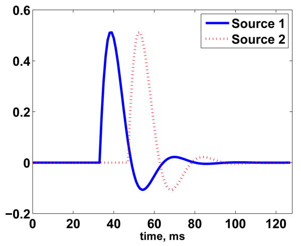
We now conduct a series of randomized simulations to illustrate the performance of the ESP procedure under various signal conditions. Two spatially extended cortical sources of activity are present in each simulation. Each source follows a damped cosine time course as shown in Fig. 12. Trials with less than about 25 ms between the onset of source 1 and source 2 exhibit temporal overlap at the sensors. For example, the onset of source 2 is 14 ms later than that of source 1 in Fig. 12 and significant temporal overlap is present. The location, size, and starting time of each source is selected at random to provide a rich variety of source configurations. Specifically, the center point of each event is selected uniformly at random from all 24514 voxels on the cortical surface. The geodesic radius of each source is selected uniformly at random between 8 and 40 mm. The amplitude of activity of each dipole in a source is given by $\text{cos}\left(\frac{1.5\mathrm{\Delta }}{r}\right)$ where Δ is the geodesic distance from the center of the source and r is the geodesic radius of the source. Finally, the onset of activity in each source is selected uniformly at random between 0 and 75 ms. The measurement period is 128 ms and the average SNR is set to 0 dB.

Fig. 12.

Example time courses (Trial 6) of cortical activity for simulations of Table 1.

ESP reconstruction is performed using the 20 mm radius spatial bases and 64 ms duration wavelet temporal bases of Sec. 3.1 with three overlapping time windows. We calculate the distance error between the center of the true source and the center of the debiased ESP estimate of that source at the peak time sample. The center is found by taking a signal energy weighted average of all active voxels. When sources overlap in time, a weighted k-means algorithm is used to separate voxels into two groups (one for each source). The source one and two SNR is defined as ${\Vert {\mathbf{\text{HX}}}_1\Vert }_F^2/E[{\Vert \mathbf{\text{N}}\Vert }_F^2]$ and ${\Vert {\mathbf{\text{HX}}}_2\Vert }_F^2/E[{\Vert \mathbf{\text{N}}\Vert }_F^2]$, respectively. These values depend on both the source spatial extent and the source location. Note that the individual source SNRs do not sum to the overall SNR of 0dB because of spatio-temporal interaction between the sources. The heuristic of Section 2.6 is used to select λ in each trial. Table 1 summarizes the results of 10 trials.

Table 1.

Randomized source scenarios and patch center distance errors for Example 2.

Trial	Source	Hemisphere	Onset (ms)	Geo. Radius (mm)	Source SNR (dB)	Distance Error (mm)
1	1	Right	67	27.4	-2.61	12.5
	2	Left	57	23.6	-3.49	6.7
2	1	Right	14	32.8	-0.20	7.1
	2	Right	53	23.7	-13.57	19.3
3	1	Right	31	36.3	-0.07	4.0
	2	Right	16	16.7	-17.09	miss
4	1	Left	50	9.7	-1.27	9.7
	2	Right	23	15.3	-5.98	15.3
5	1	Right	42	22.5	-0.73	9.3
	2	Left	28	9.2	-8.02	5.6
6	1	Right	34	19.6	-4.55	8.1
	2	Right	48	15.4	-1.60	6.9
7	1	Left	48	33.8	-0.00	5.6
	2	Right	8	8.3	-29.67	miss
8	1	Left	14	18.1	-9.52	20.6
	2	Left	30	31.6	-0.52	10.4
9	1	Left	3	18.9	-9.48	16.0
	2	Left	41	31.5	-0.48	4.8
10	1	Right	73	12.2	-8.51	10.9
	2	Right	37	23.1	-0.67	8.8

Figure 13 illustrates ESP spatial reconstruction for both sources in Trial 6. Some spatial spreading occurs around both sources. ESP identifies low level activity in the region of source 2 before the activity begins. This is a result of noise present between the edge of the active time window and the onset of activity. Figure 13(d) shows the ESP reconstruction at the time of the peak source 2 activity. This time point corresponds roughly to the second temporal peak of the source 1 activity (see Fig. 12), so activity associated with source 1 is visible.

Spatial reconstructions for Trial 8 are shown in Fig. 14. Here again spatial spreading is evident. Though the correct location is included in the solution for both sources, the peak of activity in both cases is biased.

We conclude this example with an illustration of EM algorithm convergence performance. Figure 15 shows the number of EM iterations required to find each Θˆ(λ) for all ten trials of Table 1. For nearly all trials, fewer than 50 iterations are required for λ ≥ 0.3λ_MAX.When λ = 0.1λ_MAX, about 500 iterations are required. This increase in iterations corresponds to an increase in the number of active STEs in the solution (see Fig. 1).

3.4 Self-Paced Finger Tapping Experiment

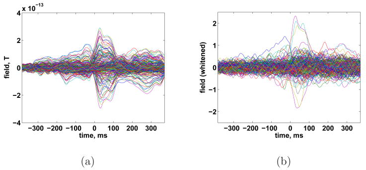
We also applied ESP to MEG measurements of a subject performing self-paced finger tapping. The data were collected with a Magnes 3600 whole head system at a sampling rate of 678 Hz and band pass filtered to lie between 2 and 40 Hz. The measured data were grouped into 80 epochs of 755 ms duration (512 samples) referenced to the tap at time 0 detected via a switch closure. Whitening was performed via Eq. (16) where R_N was estimated by removing the average response from all epochs and calculating a sample covariance matrix by averaging over time and epochs. The averaged sensor measurements before and after whitening are shown in Fig. 16. Cortical patches of 20 mm geodesic radius are used to construct the spatial bases S_i. Seven possible temporal events are represented by dividing the 755 ms measurement interval into overlapping 189 ms (128 samples) intervals. Each interval is represented using 32 wavelet bases.

Fig. 16.

Recorded MEG from self-paced finger taping. (a) Averaged data. (b) Whitened average data.

The debiased reconstruction shown in Fig. 17 is calculated using the heuristic of Section 2.6 to select λ. The estimate of activity begins about 200 ms pre-tap and persists through the end of the measurement period. The earliest activity occurs in the left motor cortex, which corresponds with the action of initiating the finger tap. The next region to become active spans the somatosensory and posterior parietal cortex. The somatosensory activity likely reflects the sensation of pushing down the switch. The posterior parietal cortex is involved in spatial relationships, body image, and movement planning (Bear et al., 2001). The parietal lobe activity begins at low levels about 100 ms before the switch closes and continues throughout the measurement period. It is possible that the early onset of activity in the parietal lobe is a result of noise in the same temporal subspace as an active time window. Beginning at about 0 ms the ESP reconstruction includes a small patch on the left frontal lobe. Some weak activity is also identified in the right hemisphere, primarily in the parietal lobe. This is consistent with earlier studies' finding that the right parietal cortex plays a role in spatial processing (Culham et al., 2006).

Fig. 17.

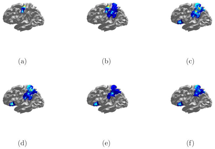
Debiased ESP reconstruction of self-paced finger taping with heuristic λ. (a) -105 ms. (b) -31 ms. (c) 28 ms. (d) 80 ms. (e) 176 ms. (f) 264 ms.

4 Discussion

The ESP approach searches for a small number of STEs which best explain the measurements. An appropriately chosen basis function representation for each STE reduces the number of parameters in the inverse problem by only representing activity that is measurable at the M/EEG sensors. Thus, our approach can incorporate the inherent limitations of the forward problem to formulate a more tractable inverse problem. The spatial bases can be chosen to represent extended sources such as patches or multipoles. The temporal basis functions naturally constrain the solution based on temporal features of interest, such as the time-frequency characteristics. Use of both spatial and temporal bases allows ESP to automatically determine both where and when significant activity occurs. A similar joint spatio-temporal philosophy based on beamforming has been proposed recently by Dalal et al. (2008).

We have illustrated the effectiveness of the ESP approach on simulated data and MEG recordings from a finger tapping paradigm. The simulated example in Sec. 3.2 shows the benefit of exploiting spatio-temporal sparsity in a three source scenario. The randomized two source scenarios in Sec. 3.3 indicate that ESP is capable of recovering almost all cortical sources with the majority of centroid localization errors less than 1 cm. The centroid localization errors are generally inversely proportional to the source SNR. In Trials 3 and 7, the weaker of the two sources was not detected using ESP due to the very low SNRs associated with these sources. In the self-paced finger tapping experiment of Sec. 3.4, ESP recovers spatio-temporal activity consistent with known brain behavior.

Our examples include source activity of varying complexity. In some cases, individual events have similar powers. Others include a weak source and a strong source. The spatial separation and temporal overlap of sources also vary. Evaluating the degradation in performance of ESP (or any other approach) as a function of increasing source complexity is an important problem. Unfortunately, quantifying this degradation is difficult, as “source complexity” can include both the number of events and the pattern of spatial and/or temporal activity of each source. We believe the use of temporal priors in the ESP approach renders it more robust to degradation due to source complexity than methods which use only spatial priors. Sources falling in different temporal subspaces are easier to separate with ESP than simple ℓ₁ spatial regularization at a single time point.

The use of sparse representations in the spatial and temporal/frequency domains for M/EEG is not unique to our approach. Sparsity in the spatial domain is enforced by limiting the number of dipolar, multipolar, patch based, or “meso-” sources used to represent measured data, usually via an ℓ₁ penalty (Auranen et al., 2005; Daunizeau and Friston, 2007; Ding and He, 2007; Gorodnitsky and Rao, 1997; Huang et al., 2006; Jeffs et al., 1987; Matsuura and Okabe, 1995, 1997; Ou et al., 2009; Uutela et al., 1999). Sparsity in the time domain has been used both implicitly and explicitly in M/EEG. One common implicit approach is to project measured data onto a few temporal basis functions derived from a singular value decomposition of the data (Huang et al., 2006; Ou et al., 2009). The more explicit approaches often involve finding a small number of wavelets which represent the signal well. This is accomplished via thresholding of wavelet coefficients (Effern et al., 2000; Trejo and Shensa, 1999) or wavelet shrinkage approaches (Trujillo-Barreto et al., 2008). A similar approach using damped sinusoids instead of wavelets is proposed in (Demiralp et al., 1998).

The ESP criterion involves the weighted combination of the squared fitting error and a penalty designed to encourage solutions consisting of a small number of STEs. The resulting cost function is convex and is minimized with a novel EM algorithm. The EM algorithm efficiently identifies a parameterized family of solutions that balance sparsity against squared error. By choosing appropriate bases and minimizing the number of STEs, ESP solutions avoid the “spiky” spatial and temporal artifacts typical of ℓ₁ methods that minimize the number of active dipoles at individual time instants.

We propose choosing the penalty weight by evaluating the number of STEs in the solution as the weight decreases from the maximum value. The number of STEs increases relatively slowly as the weight decreases when unrepresented signal components are present, and then increases very rapidly as the weight decreases when the STEs in the solution begin to represent noise. Hence, the weight value at which the number of STEs begins to increase rapidly is a good choice. We present one automated approach for finding this value of rapid increase based on fitting a curve to the number of STEs.

The ESP approach differs significantly from recent work on ℓ₁ regularization. In most existing ℓ₁ approaches, the regularization term penalizes every active dipole via ‖vec (X) ‖₁ or, if applied in the context of a basis expansion (Eq. (4)), penalizes every active coefficient via ‖vec(Θ) ‖₁. In contrast, ESP gives a smaller penalty to active coefficients in the same block than to active coefficients in different blocks. This promotes solutions consisting of a few active spatio-temporal blocks, rather than a few active coefficients or dipoles, while accommodating uncertainty in the spatio-temporal evolution of each block. Given appropriate spatial and temporal bases for each STE, ESP favors solutions which are connected spatially and vary smoothly over time as opposed to the “spiky”, disconnected results often seen in standard ℓ₁ minimization.

The mesostate model recently proposed by Daunizeau and Friston (2007) also treats cortical activity as a collection of a small number of events, or mesosources, which are identified through a Variational Bayesian (VB) inversion. The mesostate approach differs in a number of ways from the ESP approach. First, the maximum number of meso-sources must be known a priori. In Daunizeau and Friston (2007), this number is between one and eight. Second, the VB inversion “switches off” mesostates with little or no evidence. The ESP approach, on the other hand, works by “switching on” STEs with strong evidence from a large number of candidate STEs. Third, each meso-source is described by a mean time course and spatial location. Dipoles comprising a meso-source are modeled as perturbations of this mean activity. An STE, on the other hand, describes any measurable activity occurring in a local region of space and time, and thus is not limited to representation of average activity.

Another recent source imaging method proposed by Ou et al. (2009) uses a cost function similar to our ESP cost function. Unlike our approach, Ou et al. (2009) do not exploit potential sparsity in the temporal and/or frequency domains to separate sources. Instead, the measured data is projected onto a few dominant singular vectors of the data, similar to the VESTAL approach. As a result, these bases span the entire measurement period under study. The main downside to this approach is that, unlike ESP, it can not resolve temporally localized activity (compare Figs. 6 and 9). Furthermore, the method proposed in Ou et al. (2009) decimates the mesh representing the cortex, using single dipolar sources to represent larger cortical areas. A third difference between ESP and the Ou et al. (2009) approach is the method by which the cost function is minimized. Ou et al. (2009) use second-order cone programming on problems with far fewer parameters. ESP uses an novel EM algorithm which scales linearly with problem dimensions, whereas SOCP scales cubically. SOCP approaches are computationally intractable for the problem sizes considered in this paper.

Several block penalty methods similar to our ESP approach have been proposed (Malioutov et al., 2005; Tropp, 2006; Turlach et al., 2005; Yuan and Lin, 2006), though none of them in the context of M/EEG. All of these aim to find solutions which are sparse spatially, but not temporally, i.e., are sparse in only one of the dimensions. Also, all but Yuan and Lin (2006) construct blocks containing only a single spatial basis repeated over multiple time samples. This corresponds to defining blocks based on single rows of X. Malioutov et al. (2005) penalize the sum of the ℓ₂ norms of each row of the signal matrix in direction of arrival (DOA) estimation for radar. SOCP is used to perform the optimization. Both Turlach et al. (2005) and Tropp (2006) use the sum of ℓ_∞ norms as a penalty, but again consider only single rows of the signal matrix as blocks and do not employ a temporal decomposition. Turlach et al. (2005) solve a constrained version of the ESP problem via an interior point method. Tropp (2006) does not specify an optimization algorithm, but instead provides useful analysis of the properties of minimizers. Yuan and Lin (2006) suggest essentially fixed point iteration on the nonlinear functions comprising the subgradient condition for a minimizer of Eq. (6). However, they indicate that computational complexity limits their approach to small problems. None of these earlier works consider the cost function as a Bayesian likelihood, nor does there appear to be any published Expectation-Maximization approach to these “block-sparse” problems.

The choice p = 2 in Eq. (5) results in a convex optimization and appears to yield very good results. However, modifying the M-Step in Eq. (14) slightly allows solution of Eq. (5) for other values of p as well. In this case Eq. (11) is written:

$${\widehat{\mathbf{\Theta }}}^{(k)}=\text{arg}\underset{\mathbf{\Theta }}{\text{min}}\left\{{\Vert \mathbf{\Theta }-{\widehat{\mathbf{\text{Z}}}}^{(k)}\Vert }_F^2+c\mathrm{\lambda }\text{∑}_{i,j}{\Vert \text{vec}\left({\mathbf{\Theta }}_{i,j}\right)\Vert }_p\right\}$$ (20)

Exact solutions to the M-Step represented by Eq. (20) can be obtained for the cases p = 1 and p = ∞ in addition to p = 2. The Generalized Expectation-Maximization approach (Gellman et al., 2003) can be used to solve Eq. (20) for other values of p.

Using a set of spatial basis functions based on cortical patches and wavelet temporal bases, we demonstrated the effectiveness of ESP regularization on simulated cortical signals as well as data collected from a self-paced finger tapping experiment. These specific basis functions are not required to use ESP. Other methods for constructing the S_i and T_j may also prove effective in specific problems. As one example, short time Fourier bases could be used to isolate activity in different frequency bands over the same time window. Similarly, the spatial bases could be defined for patches associated with anatomically meaningful regions of the brain such as Brodmann areas.

An anatomical approach to patch design is used in the recently proposed MiMS technique (Cottereau et al., 2007). The spatial extent of each patch is chosen based on the local characteristics of the cortical surface. A multipolar expansion of fixed order is used to represent the activity from candidate patch. MiMs employs a coarse to fine strategy to identify active regions. It begins with large patches, finds a subset of active patches that best fit the data using cross validation, subdivides active patches and repeats the patch selection/subdivision process until a fitting criterion is satisfied. MiMS does not address selection of temporal areas of interest or solve for activity jointly over space and time.

The assumptions behind ESP apply to a wide range of experimental paradigms and can accommodate varying specific assumptions through the choice of basis functions. Simulated and actual MEG data suggest ESP is effective at localizing cortical activity in both space and time.

A Minimizer of Single Block Problem

We show that θ* given by Eq. (13) is the minimizer of $f(\theta )={\Vert \theta -\mathbf{\text{Z}}\Vert }_2^2+\frac{{\alpha }^2\mathrm{\lambda }}{{\sigma }^2}{\Vert \theta \Vert }_2$ using facts from the theory of subgradients (Rockafellar, 1970). A vector g is a subgradient of a convex function f(θ) at θ₀ if f(θ) − f(θ₀) ≥ g^T(θ − θ₀) for all θ. The set of all subgradients is called the subdifferential. The subdifferential generalizes the gradient; if there is only one subgradient of f(θ) at θ₀, it is the gradient. A point θ* is the global minimizer of a convex function if and only if 0 is a subgradient of f(θ) at θ*.

It is easy to see that the subdifferential of ‖θ‖₂ contains only the gradient $\frac{\theta }{{\Vert \theta \Vert }_2}$ when θ ≠ 0, and any vector g such that ‖g‖₂ ≤ 1 when θ = 0. Now consider two cases. Case 1: Suppose ${\Vert \mathbf{\text{z}}\Vert }_2>\frac{{\alpha }^2\mathrm{\lambda }}{2{\sigma }^2}$. Then ${\theta }^{\ast }=(1-\frac{{\alpha }^2\mathrm{\lambda }}{2{\sigma }^2{\Vert \mathbf{\text{z}}\Vert }_2})\mathbf{\text{z}}$ from Eq. (13). Since θ*≠0, the subdifferential of f(θ) at θ* contains only the gradient: $2\left({\theta }^{\ast }-\mathbf{\text{z}}\right)+\frac{{\alpha }^2\mathrm{\lambda }}{{\sigma }^2}\frac{{\theta }^{\ast }}{{\Vert {\theta }^{\ast }\Vert }_2}=-\frac{{\alpha }^2\mathrm{\lambda }}{{\sigma }^2{\Vert \mathbf{\text{z}}\Vert }_2}\mathbf{\text{z}}+\frac{{\alpha }^2\mathrm{\lambda }}{{\sigma }^2}\frac{\mathbf{\text{z}}}{{\Vert \mathbf{\text{z}}\Vert }_2}=0$. Thus, θ* is a minimizer of f(θ) when ${\Vert \mathbf{\text{z}}\Vert }_2>\frac{{\alpha }^2\mathrm{\lambda }}{2{\sigma }^2}$. Case 2: Suppose ${\Vert \mathbf{\text{z}}\Vert }_2\le \frac{{\alpha }^2\mathrm{\lambda }}{2{\sigma }^2}$. Then θ* = 0 from Eq. (13). Let ${\mathbf{\text{g}}}^{\ast }=\frac{2{\sigma }^2\mathbf{\text{z}}}{{\alpha }^2\mathrm{\lambda }}$ and note that g* is a subgradient of ‖θ‖₂ at 0 since ‖g*‖₂ ≤ 1. This means that $2\left({\theta }^{\ast }-\mathbf{\text{z}}\right)+\frac{{\alpha }^2\mathrm{\lambda }}{{\sigma }^2}{\mathbf{\text{g}}}^{\ast }$ is a subgradient of f(θ) at 0. To complete the proof, note that $2\left({\theta }^{\ast }-\mathbf{\text{z}}\right)+\frac{{\alpha }^2\mathrm{\lambda }}{{\sigma }^2}{\mathbf{\text{g}}}^{\ast }=-2\mathbf{\text{z}}+2\mathbf{\text{z}}=0$.

B Derivation of λ_MAX

We show that Θˆ(λ) = 0 for λ ≥ λ_MAX given in Eq. (15). We again use the theory of subgradients (Rockafellar, 1970). We first rewrite the objective function of Eq. (6) as $f\left(\theta \right)={\Vert \mathbf{\text{Y}}-{\sum }_{i,j}({\mathbf{\text{T}}}_j\otimes {\mathbf{\text{HS}}}_i){\theta }_{i,j}\Vert }_2^2+\mathrm{\lambda }{{\sum }_{i,j}\Vert {\theta }_{i.j}\Vert }_2$, where θ is a vector concatenation of all the θ_i,j, $\theta ={\left[{\theta }_{1,1}^T{\theta }_{1,2}^T\dots {\theta }_{2,1}^T\dots {\theta }_{I,J}^T\right]}^T$. The subdifferential of f(θ) at θ = 0 contains only the vectors whose (i,j)^th component is −2(T_j ⊗HS_i)^T(y − 0) + λg_i,j where ‖g_i,j‖₂ ≤ 1 for all i, j. Let ${\mathbf{\text{g}}}_{i,j}=\frac{2}{\mathrm{\lambda }}{({\mathbf{\text{T}}}_j\otimes {\mathbf{\text{HS}}}_i)}^T\mathbf{\text{y}}$ and suppose λ ≥ 2 max_i,j(T_j ⊗HS_i)^Ty. Then ‖g_i,j‖₂ ≤ 1 for all i,j and the subdifferential of f(θ) at 0 contains the all zero vector, implying that θ = 0 minimizes f(θ).

References

- Auranen T, Nummenmaa A, Hämäläinen M, Jääskeläinen I, Lampinen J, Vehtari A, Sams M. Bayesian analysis of the neuromagnetic inverse problem with ℓp-norm priors. NeuroImage. 2005;26(3):870–884. doi: 10.1016/j.neuroimage.2005.02.046. [DOI] [PubMed] [Google Scholar]
- Baillet S, Garnero L. A Bayesian approach to introducing anatomo-functional prior in the EEG/MEG inverse problem. IEEE Trans Biomed Eng. 1997;44(5):374–385. doi: 10.1109/10.568913. [DOI] [PubMed] [Google Scholar]
- Baillet S, Mosher J, Leahy R. Electromagnetic brain mapping. IEEE Signal Processing Magazine. 2001;18(6):14–30. [Google Scholar]
- Bear M, Connor B, Paradiso M. Neuroscience: Exploring the Brain. 2nd. Lippincott, Williams and Wilkins; Philadelphia, PA: 2001. [Google Scholar]
- Bolstad A, Van Veen B, Nowak R. IEEE Statistical Signal Processing Workshop. Madison, WI: Aug, 2007. Magneto-/electroencephalography with space-time sparse priors; pp. 190–194. [Google Scholar]
- Brewer J. IEEE Transactions on Circuits and Systems cas- 9. Vol. 25. 1978. Kronecker products and matrix calculus in system theory; pp. 772–781. [Google Scholar]
- Candes EJ, Tao T. Decoding by linear programming. IEEE Transactions on Information Theory. 2005;51(12):4203–4215. [Google Scholar]
- Cottereau B, Jerbi K, Baillet S. Multiresolution imaging of meg cortical sources using an explicit piecewise model. NeuroImage. 2007;38(3):439–451. doi: 10.1016/j.neuroimage.2007.07.046. [DOI] [PubMed] [Google Scholar]
- Culham JC, Cavina-Pratesi C, Singhal A. The role of parietal cortex in visuomotor control: What have we learned from neuroimaging? Neuropsychologia. 2006;44(13):2668–2684. doi: 10.1016/j.neuropsychologia.2005.11.003. [DOI] [PubMed] [Google Scholar]
- Dalal S, Guggisberg A, Edwards E, Sekihara K, Findlay A, Canolty R, Berger M, Knight R, Barbaro N, Kirsch H, Nagarajan S. Five-dimensional neuroimaging: Localization of the time-frequency dynamics of cortical activity. NeuroImage. 2008;40(4):1686–1700. doi: 10.1016/j.neuroimage.2008.01.023. [DOI] [PMC free article] [PubMed] [Google Scholar]
- Daunizeau J, Friston K. A mesostate-space model for EEG and MEG. NeuroImage. 2007;38(1):67–81. doi: 10.1016/j.neuroimage.2007.06.034. [DOI] [PubMed] [Google Scholar]
- Daunizeau J, Mattout J, Clonda D, Goulard B, Benali H, Lina J. Bayesian spatio-temporal approach for eeg source reconstruction: Conciliating ecd and distributed models. IEEE Transactions on Biomedical Engineering. 2006;53(3):503–516. doi: 10.1109/TBME.2005.869791. [DOI] [PubMed] [Google Scholar]
- Demiralp T, Ademoglu A, Istefanopulos Y, Gülçür H. Analysis of event-related potentials (erp) by damped sinusoids. Biological Cybernetics. 1998;78:487–493. doi: 10.1007/s004220050452. [DOI] [PubMed] [Google Scholar]
- Dempster A, Laird N, Rubin D. Maximum likelihood from incomplete data via the em algorithm (with discussion) Journal of the Royal Statistical Society B. 1977;39:1–38. [Google Scholar]
- Ding L, He B. Proceedings of NFSI & ICFBI. Oct, 2007. Sparse source imaging in EEG. [Google Scholar]
- Dogandži&cacute A, Nehorai A. Estimating evoked dipole responses in unknown spatially correlated noise with EEG/MEG arrays. IEEE Trans Signal Processing. 2000;48(1):13–25. [Google Scholar]
- Donoho D. De-noising by soft-thresholding. IEEE Transactions on Information Theory. 1995;41(3):613–627. [Google Scholar]
- Donoho D. For most large underdetermined systems of linear equations, the minimal ell-1 norm solution is also the sparsest solution. Communications on Pure and Applied Mathematics. 2006;59(6):797–829. [Google Scholar]
- Effern A, Lehnertz K, Fernández G, Grunwald T, David P, Elger C. Single trial analysis of event related potentials: non-linear de-noising with wavelets. Clinical Neurophysiology. 2000;111:2255–2263. doi: 10.1016/s1388-2457(00)00463-6. [DOI] [PubMed] [Google Scholar]
- Figueiredo M, Nowak R. An em algorithm for wavelet-based image restoration. IEEE Transactions on Image Processing. 2003;12(8):906–916. doi: 10.1109/TIP.2003.814255. [DOI] [PubMed] [Google Scholar]
- Gellman A, Carlin J, Stern H, Rubin D. Bayesian Data Analysis. 2nd. CRC Press; Boca Raton, FL: 2003. [Google Scholar]
- Gorodnitsky I, Rao B. IEEE Transactions on Signal Processing. 3 Vol. 45. 1997. Sparse signal reconstruction from limited data using focuss: A re-weighted minimum norm algorithm. [Google Scholar]
- Huang M, Dale A, Song T, Halgren E, Harrington D, Podgorny I, Canive J, Lewis S, Lee R. Vector-based spatial-temporal minimum l1-norm solution for meg. NeuroImage. 2006;31:1025–1037. doi: 10.1016/j.neuroimage.2006.01.029. [DOI] [PubMed] [Google Scholar]
- Jeffs B, Leahy R, Singh M. An evaluation of methods for neuromagnetic image reconstruction. IEEE Transactions on Biomedical Engineering. 1987;34:713–723. doi: 10.1109/tbme.1987.325996. [DOI] [PubMed] [Google Scholar]
- Limpiti T, Van Veen B, Wakai R. Cortical patch basis model for spatially extended neural activity. IEEE Transactions on Biomedical Engineering. 2006;53(9):1740–1754. doi: 10.1109/TBME.2006.873743. [DOI] [PubMed] [Google Scholar]
- Malioutov D, Çetin M, Wilsky A. A sparse signal reconstruction perspective for source localization with sensor arrays. IEEE Transactions on Signal Processing. 2005;53(8):3010–3022. [Google Scholar]
- Matsuura K, Okabe Y. Selective minimum-norm solutions of the biomagnetic inverse problem. IEEE Transactions on Biomedical Engineering. 1995;42(6):608–615. doi: 10.1109/10.387200. [DOI] [PubMed] [Google Scholar]
- Matsuura K, Okabe Y. A robust reconstruction of sparse biomagnetic sources. IEEE Transactions on Biomedical Engineering. 1997;44(8):720–726. doi: 10.1109/10.605428. [DOI] [PubMed] [Google Scholar]
- Mosher J, Leahy R, Shattuck D, Baillet S. Lecture Notes in Computer Science Vol 1613 Proc IPMI99. Springer-Verlag GmbH; 1999. MEG source imaging using multipolar expansions. [Google Scholar]
- Mosher J, Lewis P, Leahy R. IEEE Trans Biomed Eng. 6. Vol. 39. 1992. Multiple dipole modeling and localization from spatio-temporal MEG data; pp. 541–557. [DOI] [PubMed] [Google Scholar]
- Nolte G, Curio G. IEEE Trans Biomed Eng. 10. Vol. 47. 2000. Current multipole expansion to estimate lateral extent of neuronal activity: A theoretical analysis; pp. 1347–1355. [DOI] [PubMed] [Google Scholar]
- Ou W, Hämäläinen M, Golland P. A distributed spatio-temporal eeg/meg inverse solver. NeuroImage. 2009;44(3) doi: 10.1016/j.neuroimage.2008.05.063. [DOI] [PMC free article] [PubMed] [Google Scholar]
- Pascual-Marqui RD, Michel CM, Lehmann D. Low resolution electromagnetic tomography: a new method for localizing electrical activity in the brain. International Journal of Psychophysiology. 1994;18:49–65. doi: 10.1016/0167-8760(84)90014-x. [DOI] [PubMed] [Google Scholar]
- Rockafellar RT. Convex Analysis. Princeton University Press; Princeton, New Jersey: 1970. [Google Scholar]
- Scherg M, von Cramon D. Two bilateral sources of the late AEP as identified by a spatio-temporal dipole model. Electroencephalogr Clin Neurophysiol. 1985;62:32–44. doi: 10.1016/0168-5597(85)90033-4. [DOI] [PubMed] [Google Scholar]
- Trejo L, Shensa M. Feature extraction of event-related potentials using wavelets: An application to human performance monitoring. Brain and Language. 1999;66:89–107. doi: 10.1006/brln.1998.2026. [DOI] [PubMed] [Google Scholar]
- Tropp J. Algorithms for simultaneous sparse approximation, part ii: Convex relaxation. Signal Processing. 2006;86:589–602. [Google Scholar]
- Trujillo-Barreto N, Aubert-Vázquez, Penny W. Bayesian m/eeg source reconstruction with spatio-temporal priors. NeuroImage. 2008;39(1):318–335. doi: 10.1016/j.neuroimage.2007.07.062. [DOI] [PubMed] [Google Scholar]
- Turlach B, Venables W, Wright S. Simultaneous variable selection. Technometrics. 2005;47(3):349–363. [Google Scholar]
- Uutela K, Hämäläinen M, Somersalo E. Visualization of magnetoencephalographic data using minimum current estimates. NeuroImage. 1999;10:173–180. doi: 10.1006/nimg.1999.0454. [DOI] [PubMed] [Google Scholar]
- Van Veen B, Van Drongelen W, Yuchtman M, Suzuki A. IEEE Trans Biomed Eng. 9. Vol. 44. 1997. Localization of brain electrical activity via linearly constrained minimum variance spatial filtering; pp. 867–880. [DOI] [PubMed] [Google Scholar]
- Wagner M, Fuchs M, Kastner J. Proceedings of the 13th International Conference on Biomagnetism. Jena; Germany: Aug, 2002. Current density reconstructions and deviation scans using extended sources. [Google Scholar]
- Wagner M, Köhler T, Fuchs M, Kastner J. An extended source model for current density reconstructions. In: Nenonen J, Ilmoniemi R, Katila T, editors. Proceedings of the 12th International Conference on Biomagnetism; Espoo, Finland: Espoo: Helsinki Univ of Technology; Aug, 2000. pp. 749–752. [Google Scholar]
- Wright S, Nowak R, Figueiredo M. Sparse reconstruction by separable approximation. IEEE International Conference on Acoustics, Speech, and Signal Processing; Las Vegas, NV. 2008. [Google Scholar]
- Wu C. On the convergence properties of the em algorithm. Annals of Statistics. 1983;11:95–103. [Google Scholar]
- Yuan M, Lin Y. Model selection and estimation in regression with grouped variables. Journal of the Royal Statistical Society B. 2006;68:49–67. [Google Scholar]