Estimating 3D respiratory motion from orbiting views by tomographic image registration

Abstract

Respiratory motion remains a significant source of errors in treatment planning for the thorax and upper abdomen. Recently, we proposed a method to estimate two-dimensional (2D) object motion from a sequence of slowly rotating X-ray projection views, which we called Deformation from Orbiting Views (DOV). In this method, we model the motion as a time varying deformation of a static prior of the anatomy. We then optimize the parameters of the motion model by maximizing the similarity between the modeled and actual projection views. This paper extends the method to full three-dimensional (3D) motion and cone-beam projection views. We address several practical issues for using a cone-beam CT (CBCT) scanner that is integrated in a radiotherapy system, such as the effects of Compton scatter and the limited gantry rotation for one breathing cycle. We also present simulation and phantom results to illustrate the performance of this method.

I. INTRODUCTION

Geometric uncertainties caused by respiratory motion complicate precision in radiotherapy treatment in the thorax and upper abdomen. Although active breath control (ABC) [1] can reduce this problem, it is very uncomfortable for patients to hold their breath, especially for those with lung cancer. Treating patients under free breathing conditions can be accomplished by constructing an internal target volume, in which the treatment plann is based on a larger margin encompassing the volume the tumor may reach during breathing [2]. Another method is respiratory-gated treatment [3]. In gated methods, treatment plan is based on the tumor position at a certain respiratory phase. During the treatment, the X-ray beam is turned on in the chosen phase and turned off otherwise. No matter what kind of methods are used, knowledge of how the patients’ anatomy moves during respiration is required for designing a treatment plan.

To obtain a complete picture of the patients’ anatomy at all times during breathing, intensive work has been dedicated to four-dimensional (4D) CT imaging [4–8]. Here 4D refers to a 3D spatial field plus a one-dimensional (1D) respiratory index. Most current 4D CT imaging techniques use conventional scanners [4–6]. These methods often acquire multiple 2D slices at each table position, sort these slices into several respiratory phase bins, and then stack those slices that are within the same phase bins to form a 4D model. Due to insufficient longitudinal coverage to image an entire volume during one breathing cycle, an assumption is made that a reproducible relationship exists between the internal motion and the “phase” of some external monitoring index. Inaccurate sorting due to imperfect correlation often leads to tissue discontinuity artifacts in the reconstructed CT volumes, especially at mid-inspiration or mid-expiration phases.

It is also feasible to image the thorax using CBCT scanners that are integrated on the gantry of the linear accelerator (linac) [7, 8]. Such scanners rotate slowly, with about 1 minute per full rotation. Therefore the collected projection views over a 360° scan span several breathing cycles. One way to obtain a motion-reduced thorax CT volume is to use only the projection views in the same breathing phase for image reconstruction, as described in [7]. However, assumptions of motion reproducibility remain a limitation. Another way is to use all the projection views and implement motion-compensated reconstruction. For example, Li et al. [8] obtained a motion model by co-registering the 4D treatment planning CT images of the same patient and then incorporated the patient’s motion model into the image reconstruction process. However, a motion model derived from 4D CT data may not match the motion during a subsequent CBCT scan for two reasons. One is the possible changes of the patient’s motion pattern through time, the other one is inaccurate spatial and temporal alignment between the 4D CT data and the CBCT data.

We propose a different way to study the moving anatomy during breathing. The previous 4D CT methods all attempt to directly reconstruct a sequence of static 3D CTs through time. However, our method attempts to estimate the movement of patients’ anatomy through time. With the estimated motion, a 3D picture of the anatomy at any selected time point can be generated by deforming a static prior according to the estimated movement at that time. Our method utilizes an on-board imager (OBI) based CBCT scanner. Although this type of scanner rotates slowly, it provides a large volume coverage (e.g., a 30 × 40 cm² detector) and a high temporal sampling rate (up to 15 projection views per second). Therefore, we have explored estimating respiratory motion from a sequence of cone-beam projection views acquired during free breathing, assuming that we also have available a static prior model of the anatomy, such as a breathhold planning CT. The basic idea of this approach is to model the motion as a time varying deformation of the prior and to estimate the motion parameters by maximizing the similarity between the modeled and measured projection views. We call this method deformation from orbiting views. Our method does not bin data over the respiratory cycle, hence it reduces the tissue discontinuity artifacts in the aforementioned phase-sorting based 4D CT imaging methods. Unlike the motion compensation method proposed in [8], our motion model is estimated from the CBCT data itself hence the possible inconsistencies of 4D CT data do not exist.

We have described the general framework of DOV previously and presented preliminary 2D simulation results [9]. 3D motion estimation from cone-beam projection views brings in several practical issues that were not addressed in our previous work, such as the limited gantry range for one breathing cycle and Compton scatter contamination in cone beam systems. For recently developed cone beam CT systems for radiotherapy, the angular span for one breathing cycle is around 20° to 40°. The drawback of this small angular range is that the projection views for one breathing cycle may be less informative about the motion along certain directions. To help overcome this limitation, we add pseudo periodicity regularization to the estimator.

This paper starts with a description of the theory of DOV, including how the estimator is formed, how the penalty terms are designed and what strategies are used for this optimization problem. Simulation and experiment results are then presented and discussed.

II. THEORY

The basic idea of DOV is to estimate respiratory motion from sequential X-ray cone beam projection views. This section is focused on the estimator for DOV. The estimator includes two kinds of terms, similarity terms and penalty terms. We first briefly review the relationship between the measured datasets, introduced in [9], and propose two possible similarity metrics. We then describe the penalty terms included in the estimator: a commonly used motion roughness penalty and an aperiodicity penalty specially designed for DOV. Afterward, the optimization strategies used for finding the estimates are given.

A. The system model

The proposed motion estimation method uses two sets of data. One is a reference thorax CT volume obtained from a conventional fast CT scanner under breathhold conditions, denoted f_ref(x), x ∈ ℝ³. The other is a sequence of projection views of the same patient acquired at treatment time using a slowly rotating cone-beam system (1 minute per rotation), denoted Y_m, m = 1, ⋯, M (M is the number of projection views). We establish the relationship between the two data sets f_ref(x) and Y in this section.

We need to first address one concern about the slowly rotating cone-beam systems. Although the cone-beam scanners rotate slowly, the acquisition time of each projection view is short. For example, recently developed systems can acquire 15 frames per second, which indicates that the imaging time for each frame is less than 0.067 second. We therefore assume that the respiratory motion is negligible within each single projection view.

Let the motion during the scan be denoted as 𝒯 _θ(x; t), a time-dependent deformation controlled by parameters θ. Since the projection views and the reference volume are all from the same patient, the ideal projection views g_m can be related to f_ref in terms of the CT imaging principle through the motion as follows,

$${\mathit{g}}_m={𝒜}_{{\varphi }_m}{f}_{t_m},$$ (1)

$$f_{t_m}(\mathit{x})=f_{\text{ref}}({\mathbf{𝒯}}_{\mathit{\theta }}(\mathit{x};t_m)),$$ (2)

where 𝒜_ϕm denotes the X-ray projection [10] operator for projection angle ϕ_m, and f_tm is the deformed volume at time t_m. Combining (1) and (2), we obtain

$${\mathit{g}}_m={𝒜}_{{\varphi }_m}{f}_{\text{ref}}({\mathbf{𝒯}}_{\mathit{\theta }}(\mathit{x};t_m)).$$ (3)

However, in practice the projection views g_m are estimated from the measured photon counts Y_m, which are always degraded by noise, dominated by the Poisson effect [11]. For simplicity, we assume a monoenergetic model to describe the relationship between g_m and Y_m as follows,

$$Y_{m,n}~\text{Poisson(}{I}_{m,n}{e}^{-g_{m,n}}+S_{m,n}),$$ (4)

where I_m,n is a constant related to the incident X-ray intensity, S_m,n denotes the scatter contribution to Y_m,n and n is the detector element index. Then the projection views used for DOV can be estimated from Y_m as follows,

$${\widehat{g}}_{m,n}=\text{log}\left(\frac{I_{m,n}}{Y_{m,n}-{\widehat{S}}_{m,n}}\right).$$ (5)

In (5), I_m,n can be measured by an air scan and Ŝ_m,n is an estimate of the scatter contribution. There are a few popular ways to estimate scatter. One is to model the scatter as the convolution of a function with the primary counts. The function could be approximated by an exponential or Gaussian kernel [12]. Another way is to measure the scatter effect using a beam stop array [13]. One may also estimate the scatter by using the Monto-Carlo simulation method [14]. The DOV method can use any such scatter estimates.

We need to choose a deformation model to complete (3). Theoretically 𝒯 _θ(x; t) can be any suitable deformation model. We adopted a cubic B-spline based motion model as follows,

$${\mathbf{𝒯}}_{\mathit{\theta }}(\mathit{x};t)=\mathit{x}+{\displaystyle \sum _j{\displaystyle \sum _{\mathit{i}}{\mathit{\theta }}_{j,\mathit{i}}\beta \left(\frac{t-{\tau }_j}{{\mathrm{\Delta }}_{\mathrm{t}}}\right)\beta \left(\frac{\mathit{x}-{\mathit{x}}_{\mathit{i}}}{{\mathrm{\Delta }}_{\mathrm{x}}}\right)}},$$ (6)

where β(·) is the cubic B-spline function and β(x) the tensor product of cubic B-spline functions, τ_j and x_i the spatial and temporal knot locations, Δ_x and Δ_t control the width of the spatial and temporal basis functions respectively, and θ the knot coefficients. There are two advantages of using a cubic B-spline model. One is that the small support of the cubic B-spline function eases the computation and optimization. The other is that the density of a B-spline control grid can be locally adjusted according to the characteristics of the signal to be fitted. For example, one can place more knots at regions where the signal changes faster and less knots otherwise. Based on the motion model (6), the estimation goal is to find the motion parameters θ from the projection views ĝ_m and f_ref.

In terms of the relationship between g_m and f_ref described in (3), we construct an estimator of θ as follows,

$$\widehat{\mathit{\theta }}=\text{arg}\underset{\mathit{\theta }}{\text{min}}(\mathit{D}(\{{\widehat{\mathit{g}}}_m\},\{{\mathit{p}}_m(\mathit{\theta })\})+{\beta }_s{R}_s(\mathit{\theta })+{\beta }_t{R}_t(\mathit{\theta })),$$ (7)

where {p_m(θ)} = {𝒜_ϕm f_ref(𝒯 _θ(x; t_m))} is the modelled projection views of the warped reference volume, D(·, ·) is a data fidelity term, R_s(θ) is a motion roughness penalty term, R_t(θ) is a temporal motion aperiodicity penalty term, and β_s and β_t are scalars that control the trade-off between the three terms.

To sum up, the goal of DOV is to find the motion, a sequence of deformations through time, to match the projection views of the warped reference image to the measured projection views. It is essentially a registration problem. But unlike the traditional image registration problem, DOV works with the projection domain data and is thus more challenging. For example, a 3D image registration task is to find a 3D deformation field from two 3D images, while DOV is tasked to find k 3D deformation fields from one 3D image and n 2D projection views, where k ≥ n. Evidently, DOV attempts to estimate more unknowns from less information. Thus, regularization is essential.

B. Data fidelity term

This section elaborates on the data fidelity term in (7). We focus on the following two intensity-based metrics: weighted sum of squared differences (WSSD) and a correlation-based metric.

WSSD

The expression of WSSD is as follows,

$$\text{WSSD}(\{{\widehat{\mathit{g}}}_m\},\{{\mathit{p}}_m(\mathit{\theta })\})=\frac{1}{2}{\displaystyle \sum _{m=1}^M{\Vert {\widehat{\mathit{g}}}_m-{\mathit{p}}_m(\mathit{\theta })\Vert }_{\mathit{w}}^2.}$$ (8)

The values of the weighting factors w could be set based on a data reliability metric such as the variance. We used uniform weighting for simplicity. The estimator with the WSSD fidelity is called the penalized weighted least-square(LS) estimator.

This metric works well for registration of images from the same modality. This rule applies to DOV as well. To yield good estimates using this approach, the X-ray energies should be the same for imaging the static CT and for acquiring the cone-beam projection views. In addition to this, extra effort may be needed to correct the imaging artifacts such as Compton scatter effects, beam hardening effects, and presence of the radiotherapy table in the projection views (not present in the prior CT).

Correlation-based metric

In the correlation-based estimator, we used the negative-logarithmed correlation coefficient (NLCC) as the data fidelity metric. The expression is as follows,

$$\begin{array}{cc}\hfill & \text{NLCC}(\{{\widehat{\mathit{g}}}_m\},\{{\mathit{p}}_m(\mathit{\theta })\})\hfill \\ =\hfill & {\displaystyle \sum _{m=1}^M-\text{ln}(cor({\widehat{\mathit{g}}}_m,{\mathit{p}}_m(\mathit{\theta })))}\hfill \\ =\hfill & {\displaystyle \sum _{m=1}^M-\text{ln}}\left(\frac{{\displaystyle {\sum }_{n=1}^N(g_{m,n}-{\overline{\mathit{g}}}_m)(p_{m,n}(\mathit{\theta })-{\overline{\mathit{p}}}_m(\mathit{\theta }))}}{{{\displaystyle \left[{\displaystyle {\sum }_{n=1}^N{{\displaystyle (g_{m,n}-{\overline{\mathit{g}}}_m)}}^2}{\displaystyle {\sum }_{n=1}^N{{\displaystyle (p_{m,n}(\mathit{\theta })-{\overline{\mathit{p}}}_m(\mathit{\theta }))}}^2}\right]}}^{1/2}}\right)\hfill \\ =\hfill & {\displaystyle \sum _{m=1}^M(-\text{ln}{\displaystyle \sum _{n=1}^N(g_{m,n}-{\overline{\mathit{g}}}_m)(p_{m,n}(\mathit{\theta })-{\overline{\mathit{p}}}_m(\mathit{\theta }))}+\frac{1}{2}\text{ln}{\displaystyle \sum _{n=1}^N{(g_{m,n}-{\overline{\mathit{g}}}_m)}^2+}}\hfill \\ \hfill & \frac{1}{2}\text{ln}{\displaystyle \sum _{n=1}^N{(p_{m,n}(\mathit{\theta })-{\overline{\mathit{p}}}_m(\mathit{\theta }))}^2}),\hfill \end{array}$$ (9)

where ḡ_m is the mean value of ĝ_m and p̄_m(θ) is the mean value of p_m(θ). In this data fidelity term, we use a logarithm to separate the numerator and denominators in the expression of the correlation coefficient, which simplifies the calculation of its gradient. Because the logarithm function is increasing, the logarithm step does not change the monotonicity of the correlation coefficient function. We negate the logarithm correlation coefficient because we are minimizing the cost function in the estimator (7).

Correlation-based metrics are suitable when the intensities of the images are linearly related. In X-ray imaging, the attenuation is larger when the X-ray energy is stronger. So we may expect the correlation-based estimator can perform well even if the energy spectra used for the conventional CT scanner and the cone-beam CT scanner are not guaranteed to be identical.

C. Penalty design

This section elaborates on the penalty terms in (7).

Spatial and temporal motion roughness penalty

The motion roughness penalty discourages rapidly changing breathing motion estimates that would be unrealistical. The spatial motion roughness can be measured qualitatively by the squared differences between the displacements of adjacent voxels, and the temporal motion roughness by the squared differences between the displacements of the same voxel at adjacent time points. To simplify this term, we replaced the displacement differences by the motion parameter differences. With this simplification, this term can be expressed mathematically as

$$R(\mathit{\theta })=\frac{1}{2}{\Vert \mathit{C}\mathit{\theta }\Vert }^2,$$ (10)

where C is a differencing matrix, with a typical row having the form (⋯, 0, −1, 1, 0, ⋯) for the first-order roughness penalty and (⋯, 0,−1, 2, 1, 0,⋯) for the second-order roughness penalty. It can be shown that the second-order differencing matrix has a very similar high-pass structure to that for penalizing displacements under a cubic B-spline deformation model. By including this penalty term, the optimization is guided toward a solution with a smoother breathing motion.

Aperiodicity penalty

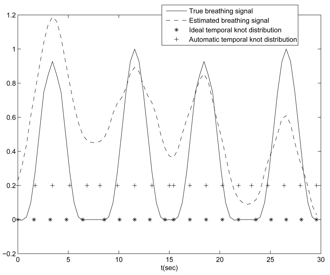
The aperiodicity penalty encourages similarity between deformation estimates that correspond to similar respiratory phases. This helps ensure temporal regularity. If the temporal knots are evenly spaced in each breathing period and each breathing period contains the same number of knots, then the deformation similarity can be quantified by the closeness of the coefficient values of knots that are located at similar respiratory phases, for the sake of simplicity. For example, in Fig. 5(solid line) there are four breathing cycles, each containing 5 locally evenly spaced knots. Thus, every fifth knot corresponds to a similar phase, such as the knot group (1,6,11, 16), the knot group (2, 7, 12, 17), and so on. Based on this design, the aperiodicity penalty term also takes the form of Eq. (10), with the matrix C having a typical row of (⋯, 0, −1, 0, ⋯, 0, 1, 0, ⋯). The number of zeros between −1 and 1 is related to the number of knots placed in each breathing period.

FIG. 5.

Ideal temporal knot placement (“*” line) and automatic temporal knot placement (“+” line)

We add this penalty term to help overcome the limited gantry range for each breathing cycle. Current radiotherapy systems can rotate 6° per second, spanning around 20 – 40° in one breathing cycle. Therefore the measured projection views in one breathing cycle may poorly reflect the motion along certain directions. For example, if the gantry starts from 0° (anterior view), then the projection views in the first breathing cycle are less informative about the AP motion, leading to poorer motion estimation accuracy along the AP direction in the absence of any other prior information. However, the projection views taken over the next breathing cycle can better capture the motion along AP direction. By using an aperiodicity penalty term, motion information contained in the adjacent breathing cycles can be “shared” to help compensate for the angular limitation.

We need a respiratory marker to determine the correspondences between the temporal knots for the aperiodicity penalty. We adopted and simplified the respiratory signal extraction method presented by Zijp’s [15]. The basic idea is to capture the SI transition of the diaphragm in the collected projection views. The method uses the following four steps:

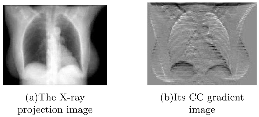
Step 1: we applied a gradient filter (e.g., h = [−1, 1]) to each 2D projection image along the Cranial-Caudal (CC) direction. This step is to emphasize the diaphragm-like transition feature in each projection image (Fig. 1).

FIG. 1.

The X-ray projection image (left) and its CC gradient image (right).

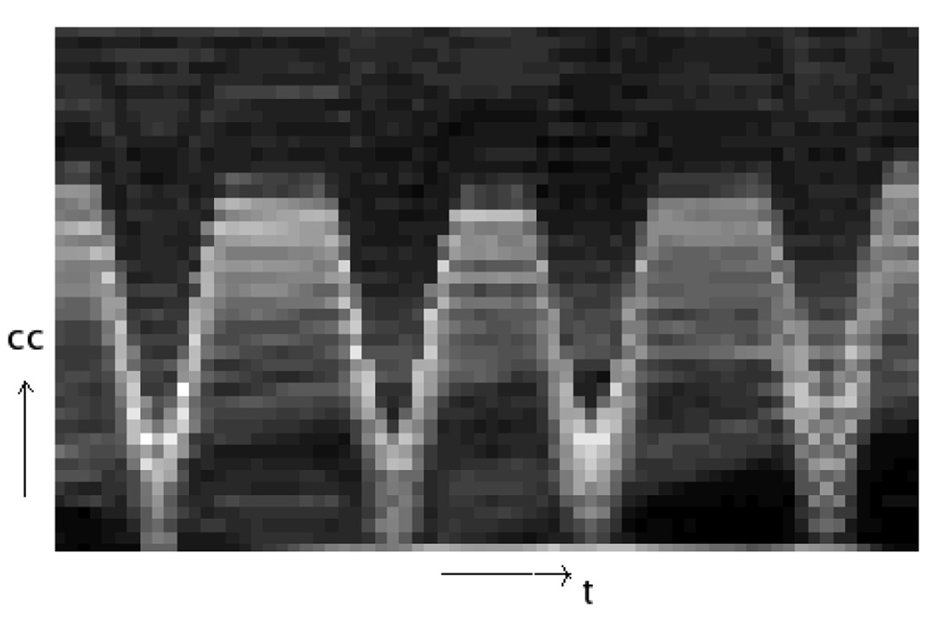
Step 2: We took the absolute value of each gradient image then projected onto the CC axis (Fig. 2). The “image” formed by combining all the 1D projections clearly shows some breathing pattern near the diaphragm region, while in the other regions there is no obvious intensity contrast (Fig. 3).

FIG. 2.

The absolute value of the gradient image (left) and its axial projection (right).

FIG. 3.

The image formed by combining the 1D axial projections. Each column corresponds to a single 1D projection.

Step 3: the centroid of each 1D projection was calculated and ordered in time. The formula for calculating the centroid of a 1D signal s_n, n = 1, ⋯ , N, is

$$\mathit{\text{centroid}}=\frac{1}{N}{\displaystyle \sum _{n=1}^{N}n{s}_n}$$

Step 4: the centroid signal was normalized and then smoothed by using a simple moving average filter.

As shown in Fig. 5, the estimated respiratory signal (dashed line) presents similar peak and valley patterns as that of the true respiratory signal (solid line). An advantage of this projection-view based method is that the resulting signal is related to internal anatomy positions, unlike external monitoring methods. We use this signal to decide the phase correspondence between temporal knots for calculating the aperiodicity penalty term. This is its only use here. Since this signal is not extremely important for the design of our motion model, a rough estimation of the breathing signal is sufficient for DOV.

D. Optimization strategies

Because there is no analytical solution for (7), we used iterative methods to search for θ̂. In our previous work we used the Levenberg-Marquardt(LM) algorithm [16]. Although LM offers fast convergence, it is impractical for 3D clinical data due to the computation of a large-sized Hessian. We then experimented with the Quasi-Newton (QN) algorithm, which approximates the Hessian by updating a preconditioning matrix. Based on our experiments, the approximation was not accurate enough to guide the optimization toward a correct direction for this optimization problem. We found that the Preconditioned Conjugate Gradient (PCG) algorithm worked better than the other two algorithms.

The PCG algorithm does not use the gradient vector directly as its search direction. It modifies the gradient search directions so that the current search direction is conjugate to all the previous search directions. This modification ensures a more efficient search over the parameter space and hence converges faster than the simple Gradient Descent algorithm. The updating scheme for each iteration n includes the following steps,

$$\begin{array}{cc}\hfill {\mathit{q}}^{(n)}& =\nabla \psi ({\mathit{\theta }}^{(n)})(\text{gradient})\hfill \\ \hfill {\mathit{p}}^{(n)}& =\mathit{P}{\mathit{q}}^{(n)}(\text{precondition})\hfill \\ \hfill {\gamma }_n& =\mathbf{\{}\begin{array}{cc}0,\hfill & n=0\hfill \\ \frac{\text{real}(\langle {\mathit{p}}^{(n)},{\mathit{q}}^{(n)}-{\mathit{q}}^{(n-1)}\rangle )}{\text{real}(\langle {\mathit{p}}^{(n-1)},{\mathit{q}}^{(n-1)}\rangle )},\hfill & n>0\hfill \end{array}\hfill \end{array}$$ (11)

$$\begin{array}{cc}\hfill {\mathit{d}}^{(n)}& =-{\mathit{p}}^{(n)}+{\gamma }_n{\mathit{d}}^{(n-1)}(\text{search direction})\hfill \\ \hfill {\alpha }_n& =\text{arg}\underset{\alpha \in ℝ}{\text{min}}\psi ({\mathit{\theta }}^{(n)}+\alpha {\mathit{d}}^{(n)})(\text{stepsize})\hfill \\ \hfill {\mathit{\theta }}^{(n+1)}& ={\mathit{\theta }}^{(n)}+{\alpha }_n{\mathit{d}}^{(n)}(\text{update}).\hfill \end{array}$$ (12)

We set P = I, which is actually the unpreconditioned case. The step size α_n is often solved by line search. To save computation time, we used only one iteration of the Newton update to find a sub-optimal step size α̂_n as follows,

$${\widehat{\alpha }}_n={\alpha }_0-\frac{\dot{\psi }({\alpha }_0)}{\ddot{\psi }({\alpha }_0)},$$ (13)

where the initial value α₀ is set to be zero to simplify the calculation. The gradient q⁽ⁿ⁾, the first derivative ψ̇(α₀) and the second derivative ψ̈(α₀) can be found from (7) using the chain rule.

To accelerate the optimization procedure and to avoid local minima, we also applied a multi-resolution technique [17].

III. SIMULATION

This section presents our simulation results. The simulated datasets were generated based on several real clinical planning CTs and the geometry of a slowly rotating cone beam CT system, and thus should reflect sufficiently realistic conditions to illustrate the performance of this method. Furthermore, in the simulations absolute truth is known, permitting quantitative evaluation.

A. Simulation setup

1. Data setup

This section describes how we generated sequential cone-beam projection views of a moving CT volume using three breathhold treatment CT volumes of the same patient at different breathing phases (0%, 20%, 60% vital capacity above tidal exhale).

We selected the thorax CT at the end of exhale (0%) as our reference volume (Fig. 4), with 192 × 160 × 60 voxels and a voxel size of 2 × 2 × 5mm³. We then generated 70 cone-beam projection views of the warped reference volumes over a 180° rotation. (The warping process is described in the next paragraph.) The simulated cone-beam system had a flat-panel detector of 180 × 200 elements of size 4 × 4mm². The source to isocenter distance and the isocenter to detector distance were 1000mm and 500mm respectively. The gantry rotated 6° per second and spanned 180° over the four breathing cycles. We used a distance-driven method [18] to calculate the projection views. To simulate realistic projection views, scatter and Poisson noise were added according to the statistical property of projection views as described in (4). We first converted the projection views from attenuation to primary photon counts. The incident intensity I_m,n in (4) used for this conversion is 10⁶ counts per ray [19]. We then applied a convolution method to generate the scatter counts, in which a normalized 2D exponential kernel with a FWHM of 4cm [12] and a scatter level of 10% was convolved with the primary photon counts. Finally we added the scatter counts and the primary counts together and degraded them by Poisson noise to obtain the noisy cone-beam projection views.

FIG. 4.

The reference thorax CT.

The respiratory motion we simulated for generating the dynamic cone-beam projection views was based on the three breathhold CT volumes (0%, 20%, 60% vital capacity). We first registered the 20% and 60% volumes to the 0% volume. Then we put the SI displacements of some voxels into the following temporal breathing motion model [20],

$$z(t)=z_0-a{\text{cos}}^6(\pi t/\tau -\pi /2),$$ (14)

where z₀ is the SI position at exhale, a is the amplitude of the motion and τ is the period of breathing cycle. Knowing the deformations at three time points and with the symmetry assumption between the motions of exhalation and inhalation, we performed cubic spline interpolation of the deformations at each voxel to form one cycle of temporally continuous breathing motion. Four breathing cycles with a total 30-seconds duration were simulated, each with different breathing periods and amplitudes. The solid line in Fig. 5 shows the simulated respiratory signal.

2. Preparation for DOV

Data preprocessing

This step obtains the projection views {ĝ_m} from the measured photon counts using (5). We estimated the scatter using the convolution method assuming the same exponential kernel as the one for generating scatter. Although we used the same exponential kernel, there was still model mismatch between the estimated and the actual scatter, as is the case in practice. The model mismatch arises from the convolution step. In data setup, we convolved the exponential kernel with the photon counts before adding noise, whereas the estimated scatter was found by convolving the kernel with the noisy photon counts.

B-spline knot distribution

The placement of B-spline control knots can be very flexible. It can be either a uniform distribution, or a nonuniform distribution. Theoretically, finer control grids enable more accurate approximation of a continuous signal. But in practice, due to the presence of noise, very fine control grids may overfit the noise. Furthermore, a finer control grid complicate optimization.

For our estimation, the control grid contained 13 × 9 × 7 spatial knots and 20 temporal knots, yielding 16380 knots in total. The spatial control knots were evenly spaced in the thorax region, with knot spacings of 16 voxels, 16 voxels and 10 voxels along the LR, AP and SI direction respectively. They were placed differently from the knot locations used for simulating the motion and with less density. The 20 temporal knots were distributed non-uniformly along the entire temporal axis, with the same number of knots evenly spaced in each active breathing period. The active breathing period is defined to be the interval from the beginning of inhale right to the end of exhale. A short rest interval follows each active breathing interval. Because the deformation during a rest interval would be very small with respect to the reference volume taken at the end of exhale, we did not place any temporal knots in this interval, reducing the number of parameters to be estimated. This nonuniform temporal knot placement facilitates establishment of the phase correspondence between knots as described in Section IIC.

Optimization setup

For optimization, the motion parameters were all initialized to be zero. We terminated the optimization algorithm when the absolute difference of the cost function value between the two most current iterations was less than a threshold. We also applied a multi-resolution technique to accelerate the optimization procedure and to avoid local minima. We started the optimization from a downsampled-by-2 version of both the reference volume and the projection views, then used the coarser-scale result as an initialization for the next finer-scale optimization. It took about 65 iterations at the coarser level and 45 iterations at the finer level to converge. The total computation time was about 10 hours using Matlab on a 3.4GHz Pentium computer.

B. Results and discussion

1. Effects of the temporal knot placement

We present two cases of results using the penalized LS estimator. One case uses an ideal temporal knot placement (“*” signs in Fig. 5), based on the true respiratory signal. The other case was with automatic temporal knot placement (“+” signs in Fig. 5) according to the estimated respiratory signal from projection views. In the former case, since the true respiratory signal was used, the phase correspondences among the knots in adjacent breathing cycles were exact and thus the periodicity regularity term could accurately align the the deformations at the same phases. The ideal case offers us a guideline on how well this proposed algorithm would perform. In the latter case, the peak intervals were detected automatically from the estimated breathing signal and temporal knots were spaced evenly in each peak intervals. Because of the mismatch between the estimated and true respiratory signals, offsets existed between the phases of the knots that were assumed to fall into the same breathing phases by the aperiodicity penalty term. This represents a practical case, where the ground truth of the respiratory signal is unavailable.

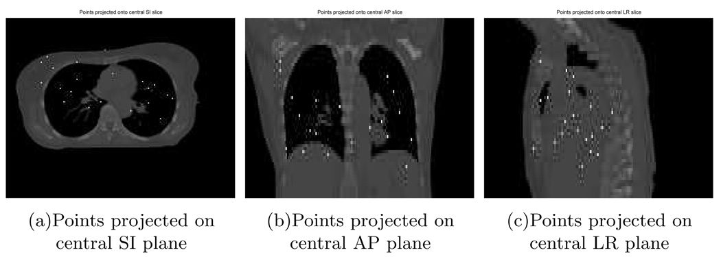
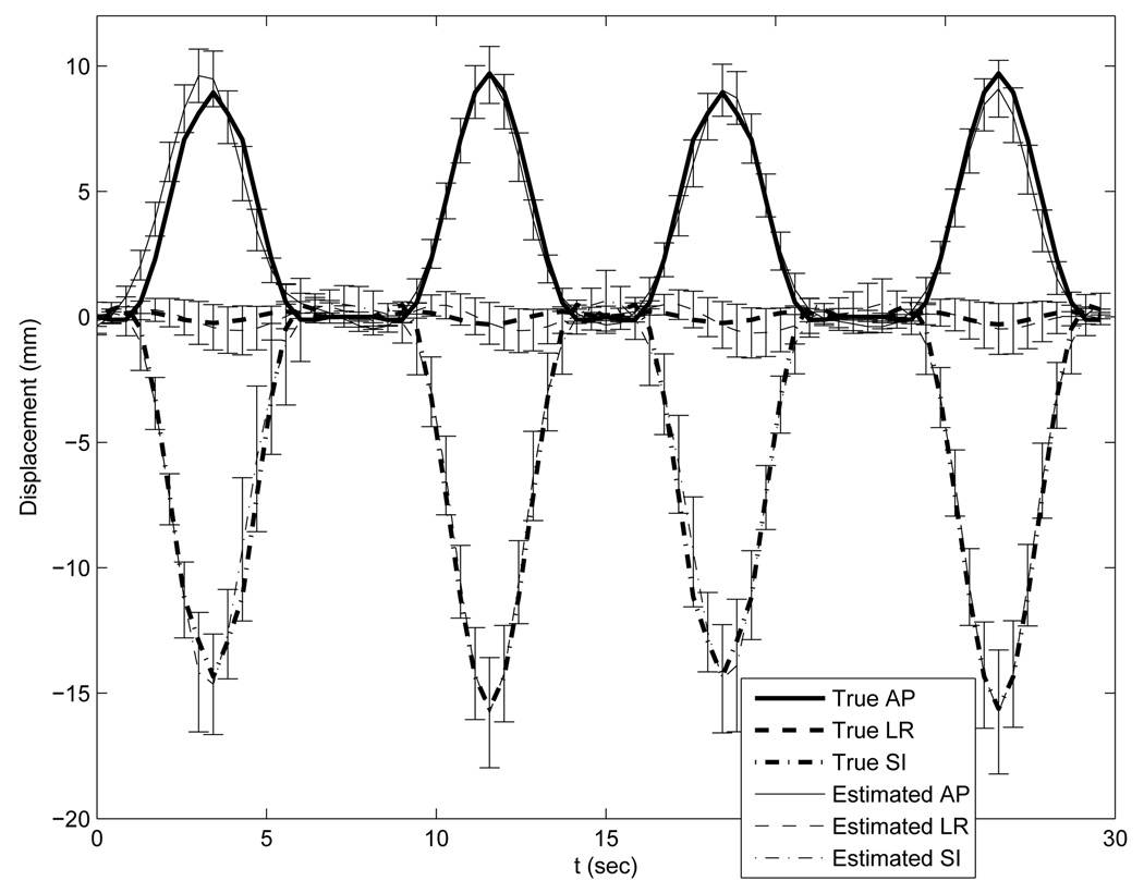
With the ideal temporal knot placement, the deformation estimation errors over the entire volume through time had nearly zero-mean Gaussian distributions. As can be seen from Table I, the standard deviations were less than 1 mm along the LR and AP direction and less than 2mm along SI. These numbers indicate that most of estimation errors were very small. The standard deviation along the SI direction was almost twice of that along the LR and AP direction due to coarser reference image sampling in the SI direction. As an example of the estimation accuracy, we plotted the averaged motion curves of 20 randomly selected points (Fig. 6) in the thorax region in Fig. 7. This plot shows good agreement between the estimated and the true motion. Slightly larger deviations from the truth occur near the peaks of the 2nd and 3rd breathing cycles for the LR motion curve and near the peaks of the 1st and 4th breathing cycles for the AP motion curve. These deviations were expected since the projection views from those angles poorly captured the deformations along the LR or AP directions respectively.

TABLE I.

Deformation estimation accuracy under ideal temporal knot placement.

	LR	AP	SI
Mean error (mm)	0.11	0.04	0.16
STD deviation (mm)	0.63	0.81	1.83
MAX Abs error (mm)	6.70	10.82	19.46

FIG. 6.

Randomly selected 20 points in thorax.

FIG. 7.

Accuracy plot of the randomly selected 20 points under the optimization with ideal temporal knot placement. The thick lines represent the true motion curves averaged over the 20 points. The thin lines represent the estimated motion curves averaged over the 20 points. Error bars on the thin lines represent the standard deviations of the deformation estimation errors.

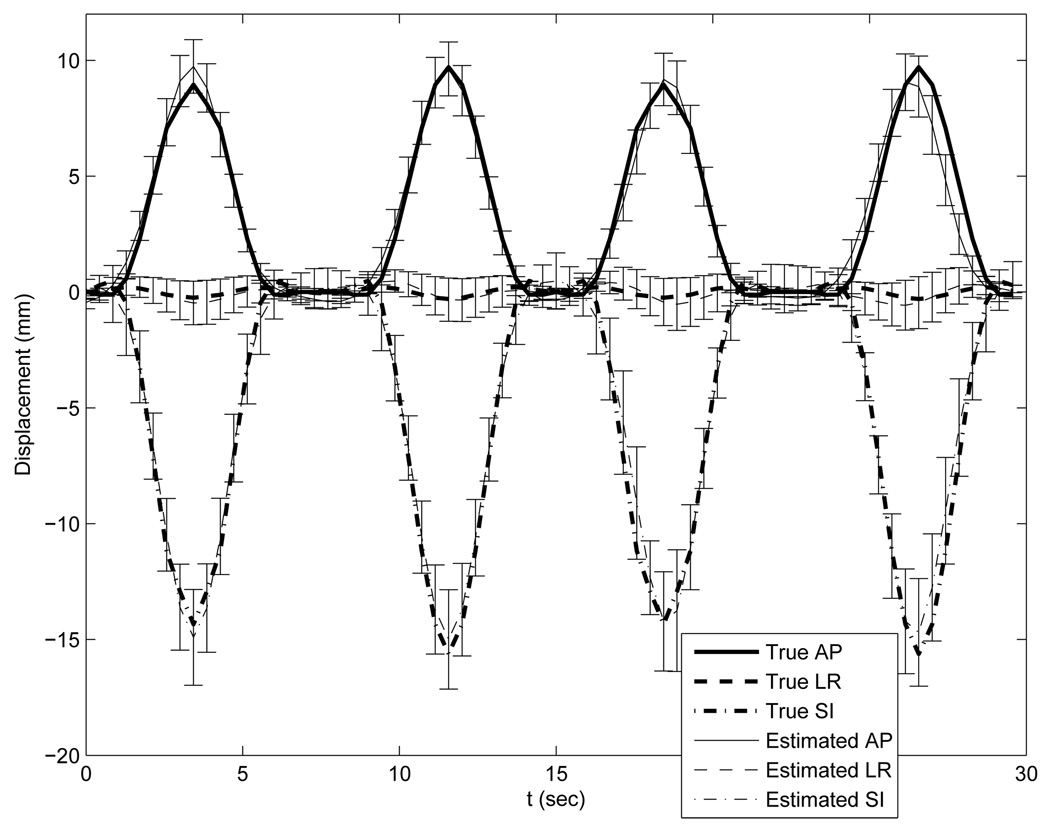
Table II lists the statistics of the deformation estimation errors with automatic temporal knot placement. Generally the estimated motion errors were slightly larger than those with the ideal temporal knot placement. Fig. 8 plots the true and estimated motion curves of the same 20 points as marked in Fig. 6. Unsurprisingly, the estimated motion curves also showed slightly larger deviation from the truth than those in the previous case. This degraded performance is mainly due to the phase offsets between knots. However, the aperiodicity penalty term did compensate for the insufficient of angular span per breathing cycle of the slowly rotating cone-beam scanner.

TABLE II.

Estimation accuracy under automatic temporal knot placement.

	LR	AP	SI
Mean error (mm)	0.12	0.06	0.27
STD deviation (mm)	0.74	0.90	2.16
MAX Abs error (mm)	8.02	9.07	23.56

FIG. 8.

Accuracy plot of the randomly selected 20 points under the optimization with automatic knot placement. The thick lines represent the true motion curves averaged over the 20 points. The thin lines represent the estimated motion curves averaged over the 20 points. Error bars on the thin lines represent the standard deviations of the deformation estimation errors.

Comparison of the two results suggests that better temporal knot placement would improve the motion estimation accuracy. Since the temporal knots are placed according to the respiratory signal, DOV would benefit from a better estimate of the respiratory signal.

Some large deformation errors did occur, even in the case of ideal temporal knot placement, e.g., a maximum absolute error of almost 10mm along the LR direction. In examining the locations of the larger errors, we found that they tended to occur in image regions having nearly uniform intensities, Because deformations in those regions would exert only very slight changes on the projection views. So these errors are likely due to a lack of image structures, which is common for registration problems.

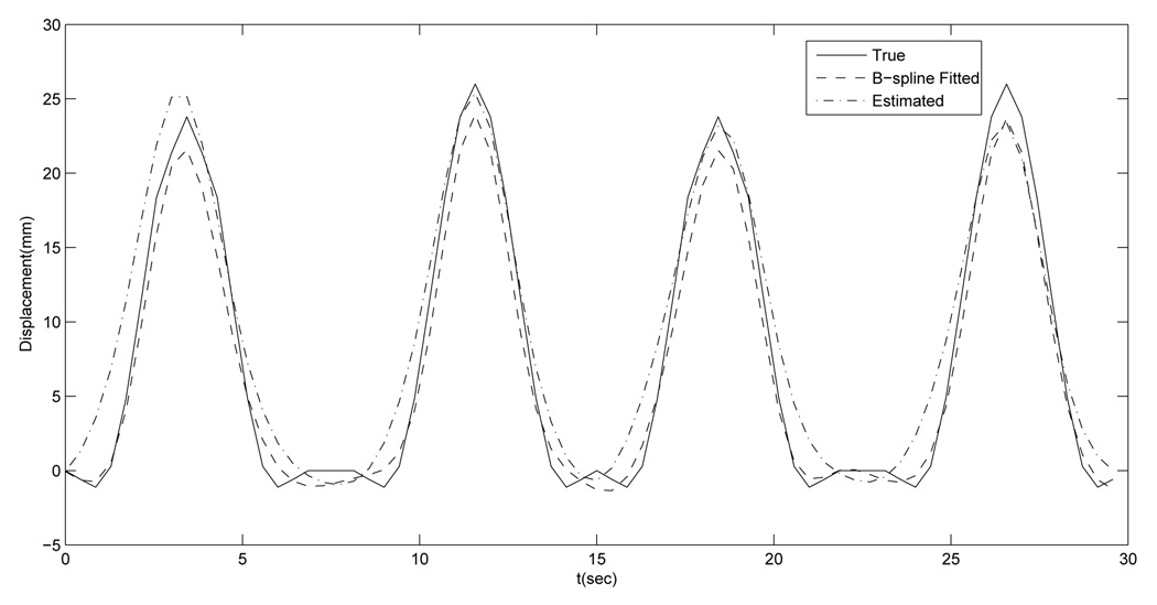
A second possible source of error is motion model mismatch, i.e., the respiratory motion could not be recovered fully by the B-spline motion model with the designed control grid. We did B-spline least square fitting of the synthetic motion using the same control grid to examine how much error would result from the model mismatch alone. Table III gives the statistics of the B-spline approximation errors. Overall the approximation errors were very small, but there were also some relatively large errors. We examined the location where the largest AP motion fitting error occurred to see how well the DOV estimation performed at that voxel. Fig. 9 compares the estimated and the fitted AP motion curves of that voxel. These two curves are close to each other, indicating that the estimated motion was close to the optimum under the selected motion model at this voxel, which did happen to be in a nonuniform region.

TABLE III.

B-spline least squares fitting error under ideal temporal knot placement.

	LR	AP	SI
Mean error (mm)	0.00	−0.01	0.00
STD deviation (mm)	0.15	0.25	0.57
MAX Abs error (mm)	3.81	4.02	9.48

FIG. 9.

AP motion curves of the voxel where the maximum B-spline fitting error along AP direction occurs: the true (solid line), the B-spline fitted (dashed line) and the estimated by DOV (dashed dot line).

2. Effects of the aperiodicity penalty

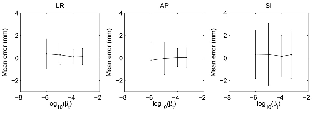
The aperiodicity penalty is important for DOV because of the limited gantry angles in one breathing cycle. A too small β_t may not sufficiently bring the motion information from the adjacent breathing cycles to compensate this limitation, while a too large β_t may subdue the role of the local motion information. This is a tradeoff. To study the impact of this term, we ran DOV using the penalized LS estimator with different β_t values and plotted the estimation accuracy in Fig. 10. As β_t increases from 10⁻⁶, the mean errors and the standard deviations in each direction tend to drop and then rise again after β_t is larger than 10⁻⁴.

FIG. 10.

The mean errors and standard deviations v.s. the aperiodicity penalty parameter β_t

3. The penalized LS and the correlation-based estimator

Table IV compares the estimation accuracies of the penalized LS and the correlation-based estimator. As can be seen from the table, the two estimators perform comparably when the intensity of the modelled projection views matches those of the measured views. Fig. 11 draws the accuracy plot of the 20 points using the correlation-based estimator. This plot also resembles the accuracy plot of the penalized LS estimator in Fig. 8.

TABLE IV.

The estimation accuracy of the LS estimator and the correlation-based estimator. The mean errors and the standard deviations were calculated over the whole volume through time

		LR	AP	SI
LS	Mean error (mm)	0.12	0.06	0.27
	STD deviation (mm)	0.74	0.90	2.16
cor	Mean error (mm)	0.11	0.06	0.20
	STD deviation (mm)	0.60	0.76	1.91

FIG. 11.

Accuracy plot of the randomly selected 20 points using the correlation-based estimator with ideal temporal knot placement. The Thick lines represents the true motion curves averaged over the 20 points. The thin lines represents the estimated motion curves averaged over the 20 points. Error bars on the thin lines represent the standard deviations of the deformation estimation errors.

IV. PHANTOM EXPERIMENT

A. Phantom

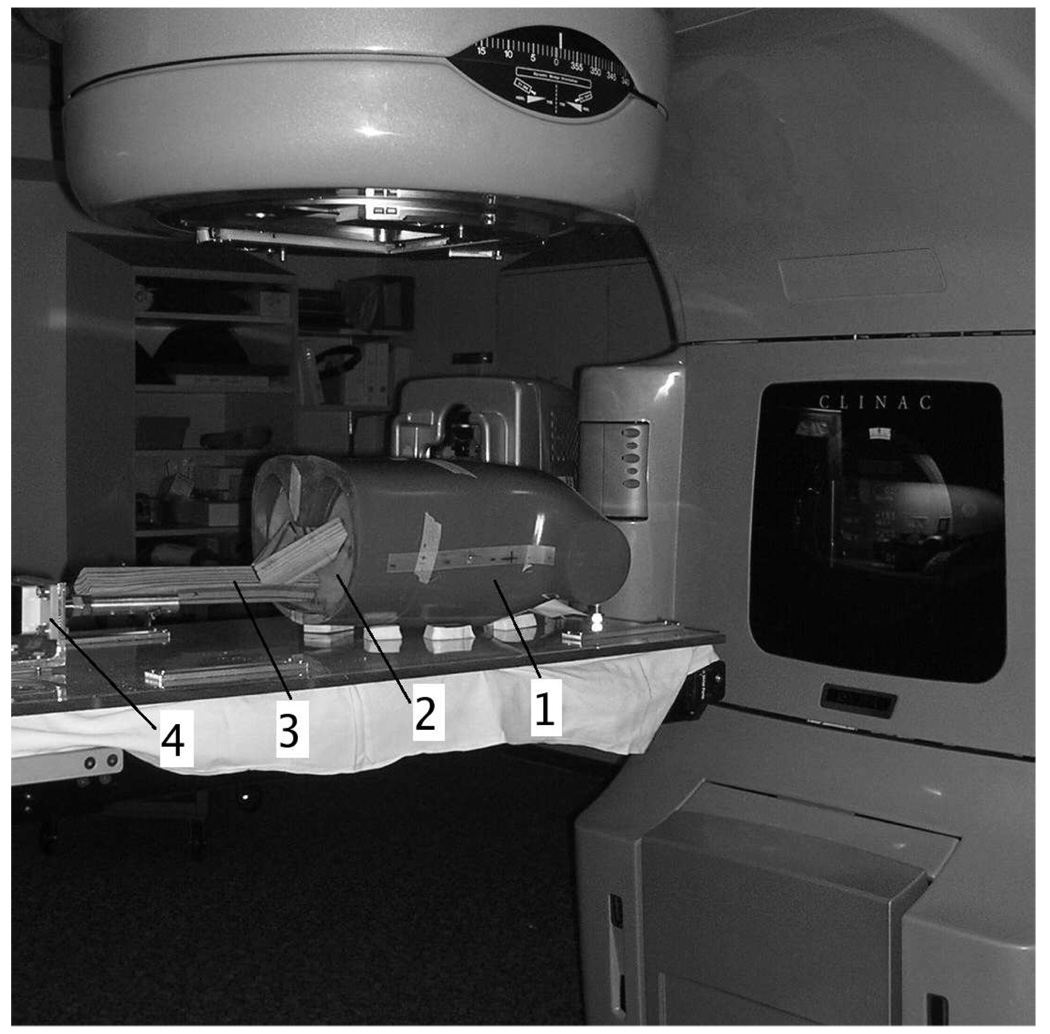
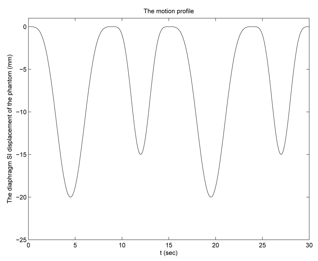
We used a partially deformable thorax phantom to test the performance of DOV, shown in Fig. 12. It is composed of a rigid frame and a compressible foam compartment inside, with some balls inserted. A rigid, flat plastic board is placed at the bottom of the phantom to simulate a diaphragm. This “diaphragm” is connected to a linear actuator through a piece of wood. Driven by the actuator, the “diaphragm” can move back and forth to compress and deform the material inside. The motion pattern of the “diaphragm” is controlled by the actuator. For this experiment, we used a motion profile with alternating amplitudes of 20 mm and 15 mm and alternating periods of 9 s and 6 s (Fig. 13).

FIG. 12.

A picture of the movable phantom: 1. the phantom; 2. the diaphragm; 3. the wood connector; 4. the actuator.

FIG. 13.

The motion profile created for the actuator.

B. Collecting data

We first scanned the phantom using a conventional CT. The voltage of the X-ray tube for this CT was set to 120kv. We scanned the phantom in three motion states, with the “diaphragm” positioned at 0cm, 1cm and 2cm toward the neck. We named the three static volumes to be CT0, CT1 and CT2 respectively. The reconstructed volumes have a size of 512 × 512 × 89 with the voxel size of 0.98 × 0.98 × 3 mm³. CT2 was used as the reference volume for DOV. The other two were used as a measure of truth to evaluate the estimation accuracy of DOV.

Then we moved the phantom to a slowly rotating cone-beam system and started the actuator and took a 360° scan of the moving phantom. Manual laser alignment was performed to set up the phantom right before starting the cone-beam scan. But instead of placing the phantom at the correct setup position, we deliberately moved the phantom off about 1 cm along the axial direction to test DOV with setup errors. After completing the cone-beam scan of the phantom, we removed the phantom and collected a full cone-beam scan of the table. The table scan was used to normalize the measured photon counts of the phantom scan. For the cone-beam scanner, the voltage of the X-ray tube was set to 125kv. The distance from the X-ray source to the detector was 1500.0mm and to the isocenter was 1000.0mm. The size of the 2D flat-panel detector was 397 × 298mm². The gantry rotated at 6° per second and 668 views were collected for a full rotation.

C. Preprocessing

We cropped the reference CT and downsampled it by 2 in the axial plane. After cropping and downsampling, the size of the reference CT was 192×180×89 and the voxel size was 2.0×2.0×3mm³. Fig. 14 shows three sides of the CT volume. The intensity of the measured projections from the CBCT scanner are linear to the photon counts. We needed to convert the counts to attenuation. The conversion was done by taking logarithm of the table scan divided by the phantom scan, i.e.,

$$\mathit{\text{attenuation}}=\text{ln}\frac{\mathit{\text{the table scan}}}{\mathit{\text{the phantom scan}}}$$ (15)

An advantage of using the table scan rather than an air scan as a normalization factor is that the table artifact may be greatly removed from the phantom scan. However, the table artifact can not be totally removed, (as can be seen in Fig. 15), because the scatter and beam-hardening effects were different in the table scan and phantom scan. For the purpose of DOV, we only used the views in the first 180° interval and downsampled them by 4 in the temporal axis, so there were about 80 views spanned over 180° used by DOV. The projection views were truncated since the 2D detector was not large enough to cover the whole width of phantom.

FIG. 14.

The phantom CT.

FIG. 15.

Cone-beam projection views at angles 181.7°, 95.7°, 29.0°

Before running DOV, we estimated the setup difference between the conventional CT and the cone-beam CT system. Without setup correction, the estimated motion by DOV would compensate for the setup errors which do not belong to the real organ motion caused by breathing. Usually a rigid setup difference is assumed. It can be described by six parameters {ϕ_x, ϕ_y, ϕ_z, t_x, t_y, t_z}: three rotation angles and three translations along each axis respectively. These parameters can be estimated by aligning the computed projection views of the reference volume to a few measured projection views. This method belong to the field of 2D-3D registration which is commonly used for setup correction in radiotherapy [21, 22]. Usually the projection views used in those registrations do not include organ motion. However, this is not the case for the collected projection views in DOV. To meet the consistency requirement, the setup difference estimation used several projection views approximately corresponding to the motion phase of the reference volume. The correspondence can be established based on the extracted breathing signal from the diaphragm transition. Correlation-based metric was used in the registration. The estimated setup difference was {0.0001rad, 0.0038rad, 0.0061rad, 0.89mm, − 0.02mm, 7.74mm}.

D. Results

Since the energies of the X-ray tubes were different for acquiring the static reference CT and the cone-beam projection views, the intensities of the modelled projection views of the reference CT did not exactly match those of the measured projection views. Furthermore, other artifacts exist in the measured views such as the scatter and beam hardening effects. Using the penalized LS estimator would involve an mapping of the 120kv reference CT to a 125kv CT. To avoid this complexity, we chose the correlation-based estimator.

The precise motion of the interior of the phantom was unknown. To evaluate the estimated motion accuracy, we established a “ground truth” using the following landmark method. We located five landmarks in the reference volume CT2 and found their displacements at two motion phases (0cm and 1cm of the “diaphragm” movement) by registering CT2 to CT0 and CT1. The landmarks we selected were the centers of five balls inserted in the phantom. (some balls can be seen in Fig. 14(b)). We assumed the registration results to be true and compared the estimated motion of the landmarks at the three phases to the truth. The motion phase associated to each cone-beam projection view can be decided by the motion profile (Fig. 13). From the motion profile, we identified that t = 3.2, 17.5s corresponded to 0cm position (CT0), t = 4.7, 9.3, 11.1, 15.7s corresponded to 1cm position (CT1) and t = 6.8, 7.2, 7.5, 12.9, 13.2, 13.6, 21.1, 21.5, 21.8s corresponded to 2cm position (CT2).

We calculated the mean errors and the standard deviations of the estimated deformations of the five landmarks at those 15 time points. The results were listed in Table V. In general, the errors were within around the resolution of one voxel. Only the systematic error in the AP direction was slightly larger than expected. Explanation of this slightly larger systematic AP error requires further investigation. We realize that the established “ground truth” may be slightly rough. In the near future, we expect to design a finer ground truth to test the DOV performance, for example, by acquiring more static CTs to find a more precise phantom motion.

TABLE V.

DOV estimation accuracy of the phantom experiment.

	LR	AP	SI
Mean error (mm)	0.4	1.1	0.2
STD deviation (mm)	2.5	2.2	1.7

E. Discussion

Although the estimation accuracy is expected to be improved furthe, the phantom experiment did illustrate the feasibility of the DOV principle, because this experiment reflected the realistic situations in the following three points of view. First, the movable phantom imitated a real human thorax. Second, a slowly rotating cone-beam CT scanner integrated in a radiotherapy simulator was used to collect the projection views, in which real imaging artifacts existed such as the truncated views, the presence of radiotherapy table, Compton scatter and beam-hardening effects. Third, setup differences between the conventional CT scanner and the cone-beam CT scanner were also considered.

However, the motion pattern of the phantom we created may be simplified compared to the true breathing motion, which would be much more irregular in both amplitude and period. This irregularity may bring uncertainty in selecting the aperiodicity penalty parameter β_t. In our phantom experiment, β_t was set to be 10⁻⁴, the value that yielded the best estimation in the simulation, because the motion patterns of the phantom and the simulation were similar. In a real patient study, a monitor may be used to instruct patients to breathe in a more regular way to reduce the difficulty in selecting β_t.

Although the phantom motion pattern was simple, the spatial deformations of the phantom included intensive “sliding” between the edge of the “diaphragm” and the interior side of the body frame. This kind of deformation is challenging to fit by the pure B-spline model. In real patients, this “sliding” phenomenon would be somewhat reduced. Therefore we may expect better estimation accuracy in a real patient case.

Due to a large angle of the X-ray cone and the use of a 2D detector, substantial scatter effects were present in the collected cone-beam projection views. In our current phantom experiment, scatter correction was skipped. This step will be implemented in the near future. We can either build a beam stop array, or experiment to find a suitable scatter convolution kernel. We believe that the DOV accuracy can be further improved with accurate scatter correction.

The estimated deformation errors for the phantom experiment were largely around the resolution of one voxel. Smaller errors can be expected using a reference volume with a higher resolution. In this experiment, we applied a multi-resolution technique and used the downsampled-by-2 reference volume at our finest-level optimization. We did not increase the resolution to that of the oringinally acquired CT volume to save computation time. We realize that the long computation time will limit the usage of the DOV method in clinic. The bottleneck of the computation is evaluating (3) and (2), the 3D deformed reference volumes and their projection views at each time points. Since most of the computation can be implemented separately view by view, the computation time can be reduced by parallel computing with a multi-processor CPU.

V. CONCLUSION

We propose DOV, a method to estimate respiratory motion from a sequence of slowly rotating X-ray cone-beam projection views. In this method, we adopt a B-spline motion model, deform a breathhold thorax CT volume according to the motion model, and find the parameters of the motion model by optimizing the similarity between the measured projection views and the modeled projection views of the deformed reference volume. There are a few advantages of this method over the other 4D CT imaging techniques. First, we do not assume any reproducibility between the internal motion and an external monitoring index, hence tissue discontinuity artifacts can be removed in the 4D CT images generated by DOV. Although we use periodicity regularization in our cost function to compensate for the limited angular range over one breathing cycle, the regularization is different from and much weaker than the reproducibility requirement. Second, the B-spline motion model gives a continous representation of the estimated motion once the motion parameters are solved. It is much more memory efficient to store only the motion parameters and a reference volume than to store a whole sequence of volumes. Third, motion is estimated from the on-board cone-beam projection data and can provide the latest update of the patient’s motion pattern.

Our simulation and phantom experiment yielded encouraging results. Performance may be further improved by using a more robust similarity metric such as Mutual information(MI) and by improving scatter correction. Better spatial knot placement may also be determined through the registration of two breathhold CT volumes. We also realize that real patient motion could not be totally charaterized by simulations or physical phantoms. Therefore, pending research will focus on further improving the estimation accuracy and applying this method to clinical cone-beam data from patients undergoing radiation therapy treatments.

References

- 1.Wong JW, Sharpe MB, Jaffray DA, Kini VR, Robertson JM, Stromberg JS, Martinez AA. The use of active breathing control (ABC) to reduce margin for breathing motion. Int. J. Radiat. Oncol. Biol. Phys. 1999 July;44(4):911–919. doi: 10.1016/s0360-3016(99)00056-5. [DOI] [PubMed] [Google Scholar]
- 2.Shih HA, Jiang SB, Aljarrah KM, Doppke KP, Choi NC. Internal target volume determined with expansion margins beyond composite gross tumor volume in three-dimensional conformal radiotherapy for lung cancer. Int. J. Radiat. Oncol. Biol. Phys. 2004 October;60(2):613–622. doi: 10.1016/j.ijrobp.2004.05.031. [DOI] [PubMed] [Google Scholar]
- 3.Starkschall G, Forster KM, Kitamura K, M D, Cardenas A, Tucker SL, Stevens CW. Correlation of gross tumor volume excursion with potential benefits of respiratory gating. Int. J. Radiat. Oncol. Biol. Phys. 2004;60(4):1291–1297. doi: 10.1016/j.ijrobp.2004.07.707. [DOI] [PubMed] [Google Scholar]
- 4.Vedam SS, Keall PJ, Kini VR, Mostafavi H, Shukla HP, Mohan R. Acquiring a four-dimensional computed tomography dataset using an external respiratory signal. Phys. Med. Biol. 2003 January;48(1):45–62. doi: 10.1088/0031-9155/48/1/304. [DOI] [PubMed] [Google Scholar]
- 5.Low DA, Nystrom M, Kalinin E, Parikh P, Dempsey JF, Bradley JD, Mutic S, Wahab SH, Islam T, Christensen G, Politte DG, Whiting BR. A method for the reconstruction of four-dimensional synchronized CT scans acquired during free breathing. Med. Phys. 2003 June;30(6):1254–1263. doi: 10.1118/1.1576230. [DOI] [PubMed] [Google Scholar]
- 6.Pan T, Lee T-Y, Rietzel E, Chen GTY. 4D-CT imaging of a volume influenced by respiratory motion on multi-slice CT. Med. Phys. 2004 February;31(2):333–340. doi: 10.1118/1.1639993. [DOI] [PubMed] [Google Scholar]
- 7.Sonke J-J, Zijp L, Remeijer P, Herk M. Respiratory correlated cone beam CT. Med. Phys. 2005 April;32(4):1176–1186. doi: 10.1118/1.1869074. [DOI] [PubMed] [Google Scholar]
- 8.Li T, Schreibmann E, Yang Y, Xing L. Motion correction for improved target localization with on-board cone-beam computed tomography. Phys. Med. Biol. 2006 January;51(2):253–268. doi: 10.1088/0031-9155/51/2/005. [DOI] [PubMed] [Google Scholar]
- 9.Zeng R, Fessler JA, Balter JM. Respiratory motion estimation from slowly rotating X-ray projections: Theory and simulation. Med. Phys. 2005 April;32(4):984–991. doi: 10.1118/1.1879132. [DOI] [PubMed] [Google Scholar]
- 10.Macovski A. Medical imaging systems. New Jersey: Prentice-Hall; 1983. [Google Scholar]
- 11.Erdoğan H, Fessler JA. Monotonic algorithms for transmission tomography. IEEE Trans. Med. Imag. 1999 September;18(9):801–814. doi: 10.1109/42.802758. [DOI] [PubMed] [Google Scholar]
- 12.Love LA, Kruger RA. Scatter estimation for a digital radiographic system using convolution filtering. Med. Phys. 1987 March;14(2):178–185. doi: 10.1118/1.596126. [DOI] [PubMed] [Google Scholar]
- 13.Ning R, Tang X, Conover D. X-ray scatter correction algorithm for cone beam CT imaging. Med. Phys. 2004 May;31(5):1195–1202. doi: 10.1118/1.1711475. [DOI] [PubMed] [Google Scholar]
- 14.Colijn AP, Beekman FJ. Accelerated simulation of cone beam X-ray scatter projections. IEEE Trans. Med. Imag. 2004 May;23(5):584–590. doi: 10.1109/tmi.2004.825600. [DOI] [PubMed] [Google Scholar]
- 15.Zijp L, Sonke J-J, Herk M. Extraction of the respiratory signal from sequential thorax cone-beam X-ray images. Proc. Intl. Congr. Comp. in Radiotherapy. 2004 [Google Scholar]
- 16.Press WH, Flannery BP, Teukolsky SA, Vetterling WT. Numerical recipes in C. New York: Cambridge Univ. Press; 1988. [Google Scholar]
- 17.Thevenaz P, Unser M. Optimization of mutual information for multiresolution image registration. IEEE Trans. Im. Proc. 2000 December;9(12):2083–2099. doi: 10.1109/83.887976. [DOI] [PubMed] [Google Scholar]
- 18.De Man B, Basu S. Distance-driven projection and backprojection in three dimensions. Phys. Med. Biol. 2004 June;49(11):2463–2475. doi: 10.1088/0031-9155/49/11/024. [DOI] [PubMed] [Google Scholar]
- 19.Whiting BR, Montagnino LJ, Politte DG. Modeling X-ray computed tomography sinograms. 2001 submitted to mp. [Google Scholar]
- 20.Lujan AE, Larsen EW, Balter JM, Ten Haken RK. A method for incorporating organ motion due to breathing into 3D dose calculations. Med. Phys. 1999 May;26(5):715–720. doi: 10.1118/1.598577. [DOI] [PubMed] [Google Scholar]
- 21.Kim J, Fessler JA, Lam KL, Balter JM, Ten Haken RK. A feasibility study of mutual information based set-up error estimator for radiotherapy. Med. Phys. 2001 December;28(12):2507–2517. doi: 10.1118/1.1420395. [DOI] [PubMed] [Google Scholar]
- 22.Weese J, Penney GP, Desmedt P, Buzug TM, Hill DLG, Hawkes DJ. Voxel-based 2-D/3-D registration of fluoroscopy images and CT scans for image-guided surgery. IEEE Tr. Information Technology in Biomedicine. 1997 December;1(4):284–293. doi: 10.1109/4233.681173. [DOI] [PubMed] [Google Scholar]