Multi-dimensional Liquid Chromatography in Proteomics

Abstract

Proteomics is the large-scale study of proteins, particularly their expression, structures and functions. This still-emerging combination of technologies aims to describe and characterize all expressed proteins in a biological system. Because of upper limits on mass detection of mass spectrometers, proteins are usually digested into peptides and the peptides are then separated, identified and quantified from this complex enzymatic digest. The problem in digesting proteins first and then analyzing the peptide cleavage fragments by mass spectrometry is that huge numbers of peptides are generated that overwhelm direct mass spectral analyses. The objective in the liquid chromatography approach to proteomics is to fractionate peptide mixtures to enable and maximize identification and quantification of the component peptides by mass spectrometry. This review will focus on existing multidimensional liquid chromatographic (MDLC) platforms developed for proteomics and their application in combination with other techniques such as stable isotope labeling. We also provide some perspectives on likely future developments.

1. Introduction

Proteins, the molecular product of genes, are vital to living organisms as they comprise the machinery required for operation of metabolic pathways. Protein expression depends on cellular and environmental conditions, and consequently proteins are expressed at different times and under different conditions. For nearly two decades, proteomics research has attempted to provide the identity and level of expression of large numbers of proteins and protein variants in different physiological states in a cell, bodily fluids, or tissues. The expectation is that this information will inform our understanding of biological function and also provide molecular signatures for particular health and disease states. In contrast to mRNA expression analysis, proteomics indicates actual, rather than potential, functional states of a cell or a tissue. Quantitative proteomic approaches will finally foster a better understanding of disease pathogenesis and push the development of better, earlier disease diagnostics and more effective, targeted therapeutics.

1.1. Challenges in proteomics

Proteomics was initially envisioned as a technique for global characterization of all components in a proteome simultaneously. Compared with the genome, the proteome is a more dynamic system with large subject-to-subject variations. Whereas an organism's genome is more or less constant with a fixed 20,000 ∼ 30,000 human protein coding-genes, for instance, the proteome differs from cell to cell and from time to time. This is because distinct genes are expressed in distinct cell types, so that even the composition of the proteome in a cell or tissue must be independently determined. Gene expression may not correlate with protein content [1]. mRNA gene products are not always translated into protein, and the extent to which protein is produced from a given mRNA depends on the gene and on the current physiological state of the cell.

Importantly, any particular protein may go through a wide variety of alterations that critically affect its function. It is becoming increasingly clear that beyond the tens of thousands of proteins, and the extent to which proteins are expressed by most cells, many are post-translationally modified at multiple sites. Phosphorylation, glycosylation, sulfation, nitration, glycation, acylation, prenylation, methylation, proteolytic cleavage, and various forms of oxidation are some of the roughly 200 forms of post-translational modification (PTM) that can be found in proteins [2]. Combined with alternative proteins arising from mRNA splicing variation, the number of modified and unmodified proteins found in biological systems is much larger than the number of genes in an organism [3].

Another challenge in proteomics is that not all proteins are expressed at equal or even similar levels in the proteome. For example, the 12 most abundant proteins constitute approximately 95% of total protein mass of human blood. These proteins include albumin, IgG, fibrinogen, transferrin, IgA, IgM, haptoglobin, alpha 2-macroglobulin, alpha 1-acid glycoprotein, alpha 1-antitrypsin and HDL (Apo A-I & Apo A-II). If these proteins are not removed from a biological sample, the peptides generated from these proteins for proteomic analysis will compete with peptides generated from less abundant proteins during the ionization process in mass spectrometry (MS) such that the peptides generated from the low abundant proteins may not be detected by MS. Unfortunately, the majority of proteins are in the low abundance class.

It is estimated that the concentration range for protein expression levels in human cells is seven to eight orders of magnitude, rising to at least eleven orders of magnitude in human plasma [4]. However, the dynamic range of a LC-MS is about 10⁴-10⁶. For effective analysis therefore, the proteome must be fractionated to enable detection and quantification of more protein components by mass spectrometry. Current analytical strategies enable characterization of several hundreds of plasma proteins within a biological sample [5-8]. These analytical strategies include two dimensional gel electrophoresis-based or multidimensional liquid chromatography-based platforms. MS is used in both of these platforms as the last analytical step for peptide detection and protein identification.

1.2. Gel electrophoresis (GE)

The identification of proteins from complex biological matrixes has traditionally been performed using two-dimensional gel electrophoresis (2-DGE). 2-DGE separates proteins by both their isoelectric point (pI) and molecular weight. In this ‘divide-and-conquer’ strategy, proteins are resolved into discrete spots that can then be selectively excised and sequenced [9,10]. The high resolution of 2-DGE allows the researcher to pick the proteins of interest while bypassing the more abundant or less interesting proteins. It is reported that nearly 3700 discrete proteins spots on 2-DGE have been displayed [11]. 2-DGE also enables the selective sequencing of differentially expressed proteins [12-14].

Although 2-DGE is a powerful technique for protein separation, it has a number of severe limitations [15,16]. The process is difficult to automate, labor intensive, slow, and prone to contamination with unresolved proteins. The more fundamental drawbacks are a limited dynamic range for detection and the exclusion of certain protein classes, such as integral membrane proteins. Poor reproducibility is also a big problem. However, for many researchers, 2-DGE remains the preferred method for differentiating protein isoforms and post-translational modifications.

1.3. Liquid chromatography coupled with mass spectrometry (LC-MS)

So-called ‘shotgun proteomics’ utilizing LC-MS has emerged as the technique of choice for large-scale protein studies due to its superior throughput and sensitivity. In a typical shotgun proteomics experiment, a complex protein sample is enzymatically digested into peptides that are separated by high pressure liquid chromatography (HPLC), introduced into a mass spectrometer for fragmentation and sequencing to identify and quantify the parent proteins. Because of its inherent selectivity and sensitivity, LC-MS has proven to be both fast and accurate and is now the bioanalytical tool of choice for proteomics in most laboratories [17].

However, LC-MS analysis of highly complex proteomic samples remains a challenging endeavor [18,19]. The proteomic analysis is usually performed at the peptide level after sample proteolysis with trypsin (or alternative enzymes). Protein information such as identification and quantification is deduced from the detected peptides. This approach is called bottom-up proteomics. Tryptic cleavage generates multiple peptides per protein so that proteomic samples typically consist of hundreds of thousands of peptides. To date, no separation method is capable of resolving so many components in a single analytical dimension prior to the MS analysis. Consequently, multiple peptides entering the mass spectrometer at any given time can overwhelm the instrument detector. This results in a reduced number of peptide identifications, and greatly increases the LC-MS analysis variability [20]. To minimize such problems in proteomics, many research efforts have focused on the development of a more sensitive multidimensional liquid chromatography (MDLC) with higher peptide separation power [21,22]. Figure 1 outlines the general experimental work flow in MDLC-MS based bottom-up proteomics.

Figure 1.

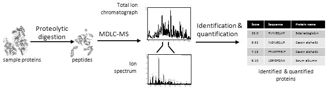
Typical bottom-up proteomics experimental workflow. Proteins are isolated from biological samples and enzymatically digested into peptides. Each protein generates many peptides (30-50 or more), which significantly increases the sample complexity. Peptides are separated using multidimensional liquid chromatography (MDLC) prior to mass spectrometry (MS) analyses. Various bioinformatics tools, such as database search algorithms, are employed for protein identification.

A major problem with bottom-up proteomics is that too many peptides are generated for direct mass spectral analysis so that it is currently not possible to achieve full protein sequence coverage. Another challenge in bottom-up proteomics is the protein inference problem. The same peptide sequence can be present in multiple distinct proteins or in protein isoforms. Such shared peptides can lead to ambiguities in determining the identities of proteins in the sample. For these reasons, an alternative approach, top-down proteomics, has attracted attention in the last few years [23-26]. In top-down proteomics, intact protein molecular ions are introduced into the mass spectrometer and subjected to gas-phase fragmentation. The top-down strategy has the potential to identify a larger fraction of protein sequences and the ability to locate and characterize PTMs. In addition, the time-consuming protein digestion required for bottom-up methods is eliminated. This not only increases the experimental efficiency, but also reduces the error rates for identification of proteins and for quantification.

However, current top-down proteomics approaches are practically limited to analysis of proteins with 500 or fewer amino acid residues (up to about 50 kDa) [27]. In addition, top-down proteomics protocols have not yet proven useful for large scale proteomics. Most MDLC systems are developed for bottom-up proteomics and this is currently the most common proteomics approach. This review will focus on MDLC systems designed for peptide separation.

2. Development of MDLC in Proteomics

As indicated, significant challenges in bottom-up proteomics are sample complexity and large concentration differences of proteins. Two main approaches have been developed to overcome these challenges. One is to develop analytical methods to separate abundant proteins from low abundance proteins, i.e., abundant protein removal (APR), to enhance the chance of detecting the latter. The other is to develop MDLC systems to either maximize the chance of MS to detect peptides present in a proteome tryptic digest by enhancing the peak capacity of the MDLC system, or to select specific fractions of peptides for analysis, often with affinity chromatography.

Abundant protein removal from complex biological samples may circumvent the large concentration differences of proteins in such samples. This is achieved largely by gel-based fractionation or immunoaffinity separation strategies [28-30]. The disadvantage of removing abundant proteins with immunoaffinity separation is that it is likely that the lower abundance proteins of interest may interact with the proteins being depleted from the sample, and thereby these will also be depleted [31].

HPLC enables full automation of sample injection, separation, detection, and fraction collection from complex biological samples. The flexibility in selecting from a variety of separation chemistries has improved the success rate for recovering classes of proteins that are difficult to handle in gel electrophoresis. An HPLC based MDLC platform can maximize the chances that the MS will detect peptides present in tryptic digest of a proteome by reducing the sample complexity prior to the MS analysis.

2.1. Principles of designing a MDLC system

In 1984, Giddings described the concept of multidimensional chromatographic separations [32]. One of the most common reasons for using MDLC in proteomics is to increase the peak capacity, i.e., the number of peaks that can be resolved at unit resolution. The mathematical definition of peak capacity in a one dimensional LC, p, for an isocratic separation (i.e., with a single and consistent mobile phase) is given as [33]

$$p=1+\frac{\sqrt{N}}{4}ln\frac{t_n}{t_A}$$

where N is the number of plates, and t_n and t_A are the times of the final peak and the void peak, respectively. It is shown that p depends upon the number of plates and upon the ratio of the retention time of the last component to that of a component that does not interact with the matrix. p can be increased by judicious choice of the length and partical size of the column and the velocity of the mobile phase.

In multidimensional separations, two or more independent separation methods are coupled in an effort to resolve complex mixtures. The resolving power of an MDLC system can be described by peak capacity P_MDLC, which is defined as the maximum number of peaks that can be resolved in a given time. In order to maximize P_MDLC, it is critical that the peptide retention mechanism in each LC dimension is orthogonal or uncorrelated, i.e., the properties affecting the separation in one dimension do not affect the separation in other distinct separation dimensions. For a completely orthogonal MDLC system, the resulting peak capacity reaches the theoretical limit given by the product of peak capacities in all dimensions, $P_{\mathit{\text{MDLC}}}^{max}=\prod p_i$, where p_i is the peak capacity in the ith LC dimension. Details of underlying theory and instrumentation employed for two dimensional liquid chromatography (2DLC) and liquid chromatography-capillary electrophoresis (LC-CE) separations are described by Evans and Jorgenson [34].

The challenge in effectively utilizing MDLC peak capacity is to find different types of LC columns that can separate peptides using uncorrelated or less correlated properties. A number of simulation studies have examined the effect of correlation on peak capacity in detail. Liu et al. developed a method that allows quantitative evaluation of orthogonality in 2D separations [35]. Solute retention parameters, such as retention times and capacity factors in both dimensions, were used to establish a correlation matrix, from which a peak spreading angle matrix was calculated with a geometric approach to factor analysis. The retention correlation calculated using solute retention vectors was used to measure the orthogonality between dimensions. It was demonstrated that most practical applications fall between the two extremes, with retention correlation values between 0 and 1. Therefore, the actual resolving power is somewhat less than that predicted from the multiplicative rule.

Gilar et al. pointed out that many MDLC systems do not have clearly demarcated zones described in Liu's work [35]. These authors proposed a binning method to identify the effective area employed over a nonuniform separation space for estimating the orthogonality, and consequently the potential peak capacity for peptides in a complex mixture [36]. This study concluded that no separation mode in 2DLC is likely to offer a complete orthogonality of separation. Rather than theoretical, the practical peak capacity of 2D separation systems should be used, taking into consideration also the number of collected fractions:

$$N_p=P_1{P}_2\frac{\sum \mathit{\text{bins}}}{P_{max}}$$

where N_p is the practical peak capacity, P₁ is the peak capacity of the first dimensional LC, P₂ is the peak capacity of the second dimensional LC, Σbins is the number of bins in a 2D plot containing data points, and P_max is the total peak capacity obtained as a sum of all bins. Using this approach, strong-cation exchange-reversed phase (SCX-RP), hydrophilic interaction chromatography (HILIC)-RP, and RP-RP 2D systems were found to provide suitable orthogonality. It is interesting that the RP-RP system (employing significantly different pH in both RP separation dimensions) had the highest practical peak capacity of the 2DLC systems investigated. In practice, peptide peaks that are well resolved on the first column may not be separated from each other on the second column due to different separation principles in the two columns. This is especially true when only a few fractions are collected from elution of the first column. Therefore, the actual peak capacity of a MDLC system is also related to the number of chromatographic fractions collected in each column.

The resolving power of a MDLC system and its efficiency are both important performance factors of a separation system for proteomics. The peak capacity value does not provide the time it takes to generate these peaks. One must also consider the rate of peak production to understand efficiency of the technique. It has been noted that peak capacities of 900 in 25 min are achievable by 2DLC; that is roughly one peak every 2 s [37]. Wang et al. developed gradient conditional peak capacity “Poppe plots” as a graphical means of assessing the compromise between conditional peak capacity and separation speed for packed bed columns [38]. These plots are especially useful for selecting the appropriate column formats (e.g. particle size and column length) in 2DLC for both the first dimension (i.e. best conditional peak capacity in a given time) and the second dimension (i.e. best conditional peak capacity production).

2.2. MDLC for analyzing tryptic digests of entire proteome

The development and use of MDLC in bottom-up proteomics has thrived over the past few years. MDLC combines two or more forms of LC to increase the peak capacity and selectivity, and thus the resolving power of separations to better fractionate peptides before they enter the mass spectrometer. In MS-based proteomics, high-resolution of peptides differing in such parameters as charge, polarity, hydrophobicity, etc., minimizes ion suppression and improves ionization efficiency. The process also simplifies the complexity of peptide ions entering the mass spectrometer to minimize under sampling. Higher MS peak capacity and better resolving power improve the acquisition of data and lead to a better representation of the proteins in the mixture.

Many multidimensional separation combinations have been reported. A variety of first dimensions, not all of them LC-based, have been used, including size-exclusion chromatography (SEC), strong cation exchange (SCX), strong anion exchange (SAX), polyacrylamide gel electrophoresis, and isoelectric focusing (IEF) techniques [39-41]. Several factors are important for the first dimension: it should have a large loading capacity, be configurable with the second dimension, and have solvent compatibility with subsequent dimensions. Some first-dimension methods are better suited for offline applications when they do not meet these criteria for compatibility with subsequent dimensions. The last separation step, typically interfaced directly to a mass spectrometer, is frequently reversed phase (RP), which can provide high resolution, effective desalting of samples, and mobile phase compatibility with electrospray ionization (ESI) and MS detection. The basis of the RP mode is hydrophobic interaction between peptides and the stationary phase. The most common stationary phase is C₁₈ covalently bound to a base silica material. Peptides are loaded onto an RP column under low-organic-solvent conditions, which permits online desalting and concentration at the same time. As the organic content in the mobile phase is gradually increased, peptides elute according to the strength of the hydrophobic interactions with the stationary support.

2.2.1. Ion exchange and reversed phase chromatography

Multidimensional protein identification technology (MUDPIT) was initially developed by Yates and his colleagues [42,43]. It uses a single biphasic microcapillary column packed first with C₁₈ RP particles and then with SCX particles to form a SCX-RP system for separation of a peptide mixture prior to analysis by mass spectrometry. Besides the differences in selectivity, the rationale for the choice of the MUDPIT separation approach is that there is good compatibility between the SCX mobile phase and the second RP separation dimension. The peptides/salt fractions from SCX can be directly introduced to the RP column; while peptides are retained on sorbent, salts are washed off the RP column.

In the MUDPIT approach, the acidified complex peptide mixture is applied to a SCX column, and a discrete fraction of the absorbed peptides is displaced onto a RP column using a salt step gradient. After washing away contaminating salts and buffers, peptides retained on the RP column are eluted from the RP column into the mass spectrometer using a gradient of increasing organic solvent concentration (typically acetonitrile). Finally, the RP column is reequilibrated in preparation for absorbing another fraction of peptides from the SCX column. An iterative process of increasing salt concentration is used to displace additional fractions of peptides from the SCX column onto the RP column. Each simplified fraction is eluted from the RP column into the mass spectrometer [42].

After the initial development of MUDPIT, several studies have been performed to improve the performance of the system. An online multidimensional LC method using an anion exchange and cation exchange mixed bed for the first separation dimension proved more orthogonal to the RP separation in two-dimensional separation, with a combination of increased retention for acidic peptides and moderately reduced retention of neutral to basic peptides by the added anion-exchange resin. This approach led to an approximately 100% increase in the number of identified peptides from an analysis of a tryptic digest of a yeast whole cell lysate [44]. Vollmer et al. applied a semi-continuous salt gradient in the first separation dimension to significantly increase the number of identified proteins from complex samples due to higher chromatographic resolution compared to stepwise elution [45]. Dai et al. used an integrated column, containing both SCX and RP sections for two-dimensional liquid chromatography [46]. The peptide mixture was fractionated with a pH step gradient, followed by reversed phase chromatography. Since no salt was used during separation, the integrated multidimensional liquid chromatography can be directly connected to mass spectrometry for peptide analysis. Winnik developed a 2D-Nano-LC/MS/MS method with continuous pH/salt gradient elution [47]. This improvement of MUDPIT is characterized by low carryover between neighboring SCX fractions and predictable SCX elution patterns, mainly dependent on the number and position of acidic and basic amino acid residues present in a peptide. Another improvement is a system that combines the SCX, SAX, and RP methods with which 14,105 unique peptides and 2,804 proteins have been identified from mouse liver [48].

2.2.2 Reversed phase - reversed phase LC (RP-RPLC)

The use of RP columns in both dimensions can be achieved either with stationary phases showing different selectivity operated with the same mobile phase [49,50], or with the same stationary phase but changing pH of the mobile phases in the two dimensions. Gilar et al. investigated two dimensional separation with reversed phase columns in both separation dimensions. The pH appears to have the most significant impact on the RP separation selectivity; the greatest orthogonality was achieved for a system with C₁₈ columns using pH 10 in the first and pH 2.6 in the second RP dimension [51]. Utilizing a RP-RP system has several advantages including high peak capacity in the first separation dimension. This permits the collection of multiple fractions with minimal content overlap. In addition, no peptide losses were observed in the first RP dimension and the mobile phases were salt free and compatible with MS detection.

An RP-RP platform based on high pressure switching between two high-resolution RP columns was implemented on an Agilent 1100 2-D liquid chromatography system, where an independent binary gradient was used for each dimension [52]. This combination achieves high analyte purity, effectively eliminates matrix effects, and maximizes MS sensitivity. Delmotte et al. developed a two-dimensional separation scheme employing high-pH reversed phase HPLC in the first and low-pH ion-pair reversed phase HPLC in the second dimension [53]. Compared to the classical strong cation exchange followed by ion-pair reversed phase approach, this system was characterized by a lower degree of orthogonality. This was, however, more than counterbalanced by higher separation efficiency, more homogeneous distribution of peptide elution, and easier experimental handling. It has also been reported that an offline coupling of a narrow-bore, polymer-based, reversed phase column using an acetonitrile gradient in an alkaline mobile phase in the first dimension with octadecylsilanized silica (ODS)-based nano-LC/MS in the second dimension identifies more peptides compared to a conventional SCX-RP system [54]. An online comprehensive RP-RP system with two parallel second dimension columns has been developed for analysis of tryptic digest of human serum [55].

2.2.3. Hydrophilic interaction chromatography (HILIC) and reversed phase LC

HILIC separation, first introduced by Alpert in 1990 [56], has increased in popularity over the last few years, promoted by the need to analyze polar compounds in increasingly complex mixtures. The separation mechanism of HILIC and the stationary phases used with HILIC have been previously reviewed [57,58]. Because of excellent mobile phase compatibility and complementary selectivity to RP chromatography, HILIC is ideally suited for highly orthogonal 2DLC separations of complex samples containing polar compounds, such as peptides and proteins. HILIC is potentially suitable for combination with RP, size-exclusion and ion-exchange chromatography.

An offline 2D-system with a sulfobetaine zwitterionic ZIC-HILIC column in the first dimension and RP chromatography in the second dimension was introduced for analysis of complex peptide mixtures [59]. The separation of peptides on the ZIC-HILIC column strongly depends on pH. At pH 3, this approach resembles SCX separations and shows high orthogonality with RP separations. At a higher pH (7–8), better chromatographic resolution is achieved, especially of prevalent +2 and +3 charged peptides in comparison to SCX separations. It is reported that an online HILIC-RP system could identify three times more peaks than the SCX-RP system in cerebral neuropeptide detection experiments, and there seemed to be no correlation between peaks detected and fraction number in the HILIC-RP method compared with most compounds eluting in the first two fractions using the SCX-RP method [60].

RP chromatography also shows complementary selectivity to HILIC on a TSK-gel^® amide column (carbamoylderivatized silica gel) in acetonitrile-rich aqueous-organic mobile phases. McNulty and Annan separated tryptic peptides on TSK-gel Amide-80 columns using a shallow inverse organic gradient. Analysis of tryptic digests from HeLa cells yielded numbers of protein identifications comparable to that obtained using SCX, and subsequent immobilized metal affinity chromatography (IMAC) enrichment of phosphopeptides from HILIC fractions showed better than 99% selectivity [61]. Another multidimensional chromatography technology combining IMAC, HILIC (TSK-gel Amide-80 columns), and RP-HPLC in sequence was developed for the purification and separation of phosphopeptides. Its application to the yeast Saccharomyces cerevisiae proteome following DNA damage led to the identification of 8,764 unique phosphopeptides from 2,278 phosphoproteins using tandem MS. This study demonstrates that HILIC provides a largely orthogonal separation of phosphopeptides when coupled with immobilized affinity chromatography (IMAC) and RP chromatography [62].

2.3. Affinity chromatography-based MDLC system (AC-MDLC)

The goal of proteomics is to detect and quantify each protein expressed in the proteome. However as we have previously noted, proteins are usually chopped into small peptides in proteomics because the MS cannot detect large molecules. Each protein may generate 20-50 peptides depending on the size of the protein and specificity of the enzyme cleavage. Measurement of multiple peptides from the same protein enhances the confidence of protein identification and quantification. However, it is not necessary to analyze every peptide digested from a protein. Detecting and measuring several peptides from one protein provides adequate information to trace back to the protein from which these peptides are generated [63]. Based on this principle, various affinity chromatography-based MDLC (AC-MDLC) systems have been developed for proteomics. Currently, there are two types of AC-MDLC systems. One is to selected low abundant peptides containing affinity selectable amino acid residues. The other is to select peptides or proteins containing certain post-translational modifications (PTMs): primarily phosphorylation and glycosylation.

2.3.1. Selection of peptides containing certain amino acid residues

In a proteome, amino acids such as leucine and serine are the most abundant at around 10% of all amino acids. At the other extreme, cysteine and histidine are relatively rare, comprising around 2% of all amino acids. Interestingly, cysteine- and histidine-containing peptides are about 10% and 17% of tryptic peptides in a proteome digest, respectively. Only about 5% of tryptic peptides contain both histidine and cysteine residues, and these are generated from about 80% of proteins [64]. These figures indicate that the majority of proteins in a proteome can be identified following enrichment of peptides based on the presence of low abundance amino acids.

Immobilized copper affinity chromatography (Cu(II)-IMAC) has been used in proteomics to simplify sample mixtures by selecting histidine-containing peptides from proteolytic digests [65-67]. An online capillary column immobilized metal affinity chromatography/electrospray ionization mass spectrometry set-up has also been reported for the selective analysis of histidine-containing peptides. The analytical cycle time in this system was reduced to less than 15 min, at an optimum flow rate of 7.5 μL/min, without sacrificing peptide selectivity [68].

Wang and Regnier developed a procedure in which cysteine-containing peptides from tryptic digests of complex protein mixtures were selected by covalent chromatography based on thiol–disulfide exchange. The cysteine-containing peptides were identified by mass spectrometry and quantified by differential isotope labeling [69]. The same group also reported a quantitative method that selects and quantifies peptides containing both cysteine and histidine residues from tryptic digests of cell lysates [66]. Cysteine-containing peptides can also be enriched by quantitatively derivatizing cysteine residues with a quaternary amine tag (QAT) [70]. Tags were introduced into disulfide bond-reduced proteins via derivatization of cysteine residues with (3-acrylamidopropyl) trimethylammonium chloride. After trypsin digestion, derivatized cysteine-containing peptides were enriched by SCX chromatography.

These and many other studies demonstrate the practicality of selection of peptides containing less abundant amino acids for proteomics. The resulting simplified peptide mixture continues to include representative peptides mapping to a very large fraction of all proteins in the proteome.

2.3.2. Selection of phosphoproteins or phosphopeptides

Quantitative analysis of protein phosphorylation provides important insights into molecular signaling mechanisms and a better understanding of many cellular processes. Various IMAC platforms have been developed for the analysis of phosphoproteins [71], in which negatively charged phosphate groups interact with positively charged metal ions (Fe³⁺, Ga³⁺, and Al³⁺). This interaction makes it possible to enrich phosphorylated peptides from complex peptide samples. A Ga(III)–IMAC has been used to select phosphorylated peptides from tryptic digests of milk [72,73]. Li et al. demonstrated the utility of iron oxide magnetic microspheres coated with gallium oxide for selective isolation and concentration of phosphopeptides prior to mass spectrometric analysis [74]. Rikard et al., compared four commercially available immobilized metal ion affinity chromatography (IMAC) methods for phosphopeptide enrichment using small volumes and concentrations of phosphopeptide mixtures with or without added bovine serum albumin (BSA) non-phosphorylated peptides [75]. The Gyros Gyrolab matrix assisted laser desorptive ionization (MALDI) IMAC1 compact disc (CD) was the most efficient method tested and could detect phosphopeptides down to low femtomole levels. Coupling stable isotope dimethyl labeling [76] with IMAC enrichment enables quantification of protein phosphorylation at MS-detected phosphorylation sites [77].

Titanium dioxide (TiO₂) chromatography has been demonstrated as an effective method for phosphopeptide enrichment [78,79]. Li et al. developed Fe₃O₄@TiO₂ microspheres with well-defined core-shell structure for highly specific purification of phosphopeptides from complex peptide mixtures to overcome the low specificity of conventional IMAC for phosphoproteome analysis [80]. This system identified 56 phosphopeptides (65 phosphorylation sites) in mouse liver lysate with a single RP-MS/MS analysis. Ahn et al. coupled TiO₂-mediated phosphopeptide enrichment and on-bead chemical labeling using a highly mass-sensitive tag, guanidinoethanethiol (GET), for phosphopeptide analysis [81]. The TiO₂ beads have high chemical stability, are physically robust and compatible with subsequent on-bead labeling processes. The introduction of the GET tag into the phosphopeptide backbone makes it possible for the GET-labeled peptides to be detected with increased mass intensity and to be efficiently sequenced in MALDI-TOF MS.

Current methods for phosphopeptide enrichment are sensitive and specific for peptide mixtures derived from pure proteins or simple protein mixtures. The selectivity and specificity of methods such as IMAC however, are limited when working with peptide mixtures derived from highly complex samples such as human plasma. Non-phosphorylated peptides contribute significantly to ion suppression of phosphopeptides, in addition to increasing sample complexity. Thingholm and Jensen suggested that lowering the pH value of the sample loading buffer significantly reduced nonspecific binding to the IMAC resin, thereby improving the selectivity of IMAC for phosphopeptides [82]. Peptide methylation can also improve the selectivity of IMAC for phosphopeptides and eliminates the acidic bias that may occur with unmethylated peptides [83]. In this approach, the IMAC procedure was significantly improved by desalting methylated peptides, followed by gradient elution of the peptides to a larger IMAC column.

2.3.3. Selection of glycoproteins or glycopeptides

Among the many types of post-translational modifications (PTMs) reported in eukaryotes, glycosylation is one of the most complex. Glycoproteins can have multiple glycosylation sites with numerous glycoforms at each site. Moreover, glycans at a particular glycosylation site can vary in both neutral and charged monosaccharide residues. Glycosylation plays fundamental roles in controlling various biological processes. Therefore, glycosylation analysis has become an important target for proteomic research and has great potential for clinical applications.

Even though glycoproteins can be analyzed using gel-based techniques [84-86], most glycoproteomics research is performed using lectin affinity approaches [87,88]. Due to the complexity of a glycoproteome, different sets of serial lectin affinity columns (SLAC) have been developed including a concanavalin A (Con A) column coupled to a sambucus nigra agglutinin (SNA) column [89], a Con A column followed by a wheat germ agglutinin (WGA) affinity column [90,91], a Con A column followed by wheat germ agglutinin (WGA) and jacalin (JAC) columns [92]. Qiu et al. have developed a nested separation system for the analysis of glycoproteins, where glycoproteins were selected with a Con A lectin column followed by trypsin digestion and sequential chromatographic selection of acidic peptides selected with a strong anion exchange (SAX) column, and histidine containing peptides selected with a copper loaded immobilized metal affinity chromatography (Cu-IMAC) column. Peptides selected by this serial process were further analyzed on RP-MS. This serial chromatography selection process reduced the complexity of proteolytic digests by more than an order of magnitude [93].

In quantitative glycoproteomics, detection of glycosylation changes could arise from concentration variations of each type of glycans or from alterations in glycan structure or glycosylation site. MALDI-TOF MS signal strength of glycopeptides has been found to accurately reflect the relative quantities of glycoforms, providing that certain technical issues are considered, i.e., nonbiased sample handling, matrix choice, and instrument settings [94]. The MS response correlates to the concentration of glycopeptides thereby enabling quantitative glycoproteomics. Many quantitative glycoproteomics studies have been reported [95-100].

The AC-MDLC approach recognizes from the beginning that existing separation technology is incapable of mapping every peptide generated from a proteome digest. AC-MDLC only targets a sub-group of peptides and therefore simplifies the complexity of the sample. On the other hand, AC-MDLC systems may focus on certain biological features of the protein, such as by selecting for certain PTMs. This approach therefore can increase the likelihood of generating biologically relevant information. However, AC-MDLC-based approaches face several challenges, not the least of which are selectivity and specificity of the affinity selectors. In addition, not all biologically important PTMs can be effectively affinity selected. In the case of glycosylation, the inability to easily differentiate between certain protein glycoforms complicates this approach, particularly for the study of diseases. Detection and quantification of every glycoform is not possible with current technologies.

2.4. Performance analysis of the existing MDLC platforms

MDLC can be implemented with the HPLC unit in either an online or offline mode. With offline operation, fractions eluted from the first column are collected by a fraction collector and then injected, either with or without concentrating the fraction, into a second column. The offline approach is simple and the mobile phases used in each column do not need to be compatible. However, the offline approach is labor intensive and time consuming, and the recovery of sample is often low. The online technique consists of the second-dimension being carried out simultaneously with the first-dimension. This system requires that the second analysis be completed during the time needed to collect the fraction, transfer and analyze it, and restore the column to the initial conditions of analysis. The online technique is advantaged by automation using electronically controlled valve systems to switch the column effluent directly from the first column into the second column. Automation improves reliability and sample throughput, shortens analysis time, and minimizes sample loss. The main limitation of the online mode is that the mobile phase system used in the two columns must be compatible in both miscibility and solvent strength.

Regardless of the mode employed, the separation achieved in the first column could be mitigated on the second column due to fraction collection. Two peptide peaks well resolved on the first column may not be separated from each other on the second column due to different separation principles in the two columns. This is especially true when only a few fractions are collected from elution of the first column, which will significantly reduce the resolving power of the MDLC system. Therefore, optimization of the MDLC system is a critical process in proteomics. The practical goal of an optimization process is either to achieve a given resolution in as short a time as possible or to reach the highest possible resolution in a given analysis time. A protocol for designing comprehensive two-dimensional liquid chromatography separation systems that establishes suitable column dimensions (length and diameters), particle sizes, flow rates, and second dimension injection volumes (i.e. loop sizes) has been described [101]. However, the recommendations made in this study cannot be readily applied in the field of proteomics due to the high flow rates, large column diameter and the fast separations performed in the second dimension. There is an optimum number of collected fractions per peak in the first dimension that provides a target peak capacity with minimum analysis time. This optimum fraction collection ratio depends on the characteristics of both the first and the second dimensions and on the target MDLC peak capacity [102]. When orthogonal columns cannot be used, the loss in peak capacity compared to a fully orthogonal system can be limited if the second dimension gradient operation is adapted to the degree of orthogonality. This can result either in an improved peak capacity or in decreasing total analysis time, depending on the final goal of the experiment [103].

With the rapid development of proteomics, multiple MDLC platforms have also been developed. Without extensive method optimization, it has been demonstrated that the online approach is preferable when very fast separations are needed. When larger peak capacities are needed, analysts must use slower methods with more powerful second separation columns, at the cost of a significant increase in the analysis time [104]. Comparative analyses report relatively minor differences in the number of proteins detected with various MDLC platforms: SCX-RP-MS/MS, high-pH SAX-RP-MS/MS and RP -RP-MS/MS (800-1200 proteins) [105]. Another comparative study showed that the online pH variance with a SCX-RP system is able to identify two times more proteins than an offline SCX-RP system [106]. However, it was also reported that the offline SCX-RP identified more proteins from human serum than the online SCX-RP [107]. Reports such as these underscore the importance of optimization of the experimental system.

The main purpose of developing MDLC systems for bottom-up proteomics is to enable more proteins to be identified and quantified by acquiring more extensive peptide information in tandem mass spectra. By way of example, Table 1 summarizes the performance of several MDLC systems for peptide and protein identification. The MDLC approach also leads to increased dynamic range of protein concentrations detected [42]. Although the dynamic range of each MDLC platform is highly dependent on experimental conditions and samples analyzed, based on our experience, we can roughly estimate the dynamic range coverage of each MDLC platform as follows: IMAC-phosphopeptide selection-RP > Lectin-glycopeptides selection-RP > IMAC-amino acid residue selection-RP > RP-RP ≥ HILIC-RP, SAX-RP, SCX-RP. However, only a small fraction of peptides generated from proteome digestion are affinity selected by an AC-MDLC system and further analyzed on MS. Many proteins identified in this approach may be represented by only one peptide. This affects the confidence for identification of the protein and may introduce a source of variation for quantitative analysis.

Table 1.

Sample MDLC proteomic studies.

Approach	Mass spectrometer	No. RP-MS analysis	Biological system	No. identified peptides	No. Identified proteins	Ref.
SCX-RP	LCQ	13	Yeast (S. cerevisiae)	5540*	1484*	42
	XCT Ultra	20	HeLa cells	5398	1283	61
	LTQ	9	Mouse liver	5779	2067	46
	Esquire HCT	44	C. glutamicum	2398	695	53
SCX-SAX-RP	LTQ	23	Mouse liver	14105	2804	48
RP-RP	Esquire HCT	31	C. glutamicum	2708	745	53
HILIC-RP	XCT Ultra	20	HeLa cells	5613	1244	61
IMAC-HILIC-RP	LTQ	20	Yeast (S. cerevisiae)	8764¥	2278¥	62

^*These are the combination of data derived from three protein fractions of cell lysate, where the tryptic digest of each protein fraction was analyzed on MUDPIT separately and the identification results from the three protein fractions were merged.

^¥These numbers refer to the number of identified phosphopeptides and phosphoprotens, respectively.

3. Application of MDLC-MS in Quantitative Proteomics

Two types of analytical platforms have been developed for quantitative proteomics [108-111], label-free and stable isotope labeling (Figure 2). Label-free quantification is a LC-MS-based method that aims to determine the differentially expressed proteins in two or more biological samples based on precursor ion signal intensity [112]. The stable isotope labeled approach introduces stable isotope signature mass tags to peptides/proteins that can be detected in the mass spectrometer to quantify each analyte and to determine the sample from which it originates [113,114]. MDLC separation coupled with mass spectrometry (MDLC-MS) is employed with both approaches to simplify peptide mixtures and to quantify and identify peptide analytes.

Figure 2.

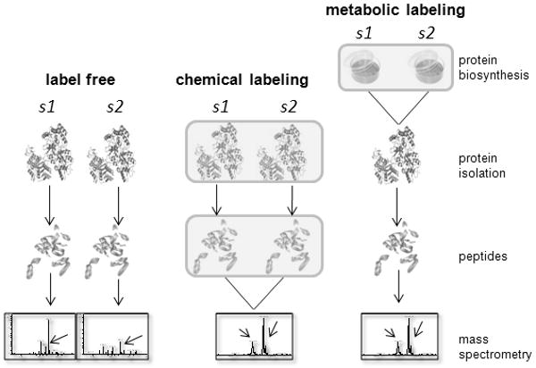
Current strategies for quantitative proteomics. In the label-free quantification approach, each sample (s1, etc.) is experimentally analyzed separately. The molecular information extracted from each sample is integrated during data analysis to obtain protein quantities (e.g., spectral counting or area under the curve calculation). Arrows in mass spectra denote differentially expressed peptides. With chemical labeling approaches, samples are labeled with various reagents either as proteins (typical for ICAT; upper box in middle panel) or as proteolytic peptides (as is typical with iTRAQ; lower box in middle panel), and mixed together prior to quantitative analysis by MS. Arrows in MS spectrum indicate an identical but differentially labeled peptide from s1 and s2. The different peak heights reflect differential levels of the parent protein. Metabolic labeling is possible with cultured cells that can incorporate labeled amino acids into proteins during growth in culture (box in right panel). Metabolically labeled samples are mixed together prior to protein isolation and further processed and analyzed by MDLC MS; quantification is again achieved via comparison of isotopically labeled peptides (as for chemical labeling approaches).

3.1. Label-free proteomics

The label-free methods have the advantage of allowing data for each sample to be acquired independently from all other samples with the expectation that samples can be compared in silico to measure changes in protein expression between conditions. This method contains three fundamental steps: sample preparation including protein extraction, reduction, alkylation and digestion; sample separation on MDLC and MS analysis; and bioinformatics including protein identification, quantification and statistical analysis.

Currently there are two widely used but fundamentally different label-free protein quantification strategies. The first of these is spectral counting in which the number of fragment spectra identifying peptides from a given protein are compared to assess relative protein abundance [115]. The second widely used label-free protein quantification strategy employs peptide chromatographic peak intensity (area-under-the-curve or AUC) measurements. In this method, chromatographic peaks of peptide precursor ions belonging to a specific protein are compared. Overall, spectral counting has proved to be a more sensitive method for detecting proteins that undergo changes in abundance, whereas peak area intensity measurements yield more accurate estimates of protein ratios [116]. Several studies have demonstrated that both spectral counting and extracted ion chromatograms (XICs) of selected peptide ions correlate well with protein abundances in complex biological samples [117-119].

The label-free strategy is simple and cost-effective with high reproducibility and linearity at both peptide and protein levels [120,121]. In general, nearly 90% of the peptide ion ratios deviated less than 20% from the average in duplicate runs in the label-free quantification approach. The removal of abundant proteins from the samples led to an improvement in reproducibility and linearity for protein quantification [120]. Given the fact that the label-free methods provide ease in experimental design well beyond pair-wise comparison, these approaches are well suited for proteomic expression profiling of large numbers of samples such as will be required for clinical analyses.

Label-free approaches coupled with MDLC system have been widely used in proteomics for global proteomic profiling [122-125]. Of note in this workflow, the final RP separation, always the last step prior to MS analysis, is a particularly time consuming process and this is amplified when large numbers of samples are analyzed. As this workflow is a sequential process, the performance of the system should be consistent throughout the entire experiment. Consequently the analyst must either spike in to each biological sample a set of internal peptide or protein standards, and/or repeatedly analyze the same biological sample to monitor the reproducibility of the analytical platform for large sample sets [126].

3.2. Stable isotope labeling based proteomics

There has been an explosion of activity in stable isotope quantification of proteins during the past few years. A wide variety of methods are available for both relative and absolute quantification of proteins. These powerful methods are designed to quantify large numbers of proteins simultaneously and the chemistry involved is relatively simple. Quantitative proteomics stable isotope labeling approaches are classified as metabolic and chemical stable isotope labeling. The metabolic labeling method attaches isotopic tags to proteins during biosynthesis [127], while the chemical stable isotope labeling approach adds isotopic tags to proteins or peptides after they have been extracted from the biological material [114]. Due to the complexity of the proteome, stable isotope labeling methods are always coupled with MDLC system for proteome quantification [68,69,76,98-100].

3.2.1. Metabolic stable isotope labeling

Most of the emphasis thus far on the metabolic stable isotope labeling has been on incorporation of a metabolic label used to identify one sample or class of samples via pair-wise comparison. For example, with two populations of cultured cells, one is fed with growth medium containing normal media while the growth medium of the second cell population contains heavy isotopes such as ¹⁸O or ¹⁵N. This cell population incorporates the heavy elements into all of their proteins. Therefore, all of the peptides that result from this culture are heavier than their normal counterparts. The two cell populations are combined and analyzed together by mass spectrometry. Pairs of chemically identical peptides with different stable-isotope composition (and therefore different masses) can be differentiated in a mass spectrometer. The ratio of peak intensities for such peptide pairs accurately reflects the abundance ratio for the proteins from which these peptides are derived. ¹⁸O- or ¹⁵N-based metabolic labeling techniques have been used in many quantitative proteomics projects [128-131]. It should be recognized however, that stable isotope incorporation rates in metabolic labeling experiments do not reach 100% [129], thereby confounding analyses.

In the stable isotope labeling by amino acids in cell culture (SILAC) technique, cells are fed with heavy isotope coded amino acids [133-135]. The amino acids used for stable isotope studies are those that are less likely to contribute isotopically labeled atoms to general metabolic pools. This requirement guarantees that the majority, if not all, stable isotope labeled amino acids will be incorporated into proteins for accurate quantification. It is also preferred that the stable isotope labeled amino acids are of high abundance in the proteome. Most studies have used leucine, followed by lysine, arginine, and to a lesser extent serine, glycine, histidine, methionine, valine, and tyrosine [136-139]. Even though most of the SILCA experiments have employed only one form of heavy-labeled amino acid [140], Mann and his colleagues developed a three-plex SILAC method. In this case, the proteomes were metabolically encoded with three stable isotopic forms of arginine to study the global dynamics of phosphotyrosine-based signaling events in early growth factor stimulation [141]. A five-plex SILAC method using four different heavy stable isotopic forms of arginine has also been developed to study the nuclear proteome and the secretome during the course of adipocyte differentiation [142].

Metabolic stable isotope labeling occurs during biosythesis. This approach avoids, or at least minimizes, technical variation that may be introduced during sample preprocessing and MDLC-MS analysis. Unfortunately, the stable isotope label in the precursor amino acids may undergo differential metabolism and thereby go undetected. In addition, this technique is currently deployed only in cell culture systems. It will be challenging to apply for human clinical studies.

3.2.2. Chemical stable isotope labeling

Isotope-coded affinity tags (ICATs) provide a versatile method for quantitative proteomics based on chemical labeling of the proteome [143]. The ICAT reagent consists of three elements: an affinity tag (biotin) used to isolate ICAT-labeled peptides; a linker that can incorporate stable isotopes; and a reactive group with specificity toward thiol groups (cysteines). The reagent exists in two forms, heavy (contains eight deuteriums) and light (contains no deuteriums). The ICAT method includes three sequential steps. It first derivatizes the side chains of cysteinyl residues in a reduced protein sample with the isotopically light form of the ICAT reagent. The equivalent groups in the second sample are also derivatized with the isotopically heavy reagent. The two samples are then combined and enzymatically cleaved to generate peptide fragments. The peptides containing cysteinyl residues are tagged. The tagged peptides are isolated by avidin affinity chromatography and separated and analyzed by LC-MS/MS. Both the quantity and sequence identity of the proteins from which the tagged peptides originated are determined by automated multistage MS. Peptides are quantified by measuring in the full MS mode the relative signal intensities for pairs of peptide ions of identical sequence tagged with the isotopically light or heavy forms of the reagent, respectively. These ions differ by the mass differential encoded within the ICAT reagents.

Although ICAT has been widely used for proteome quantification, the popularity of this approach has waned because of concerns about the isotopic effect caused by the placement of multiple deuterium atoms relative to hydrophilic functional groups in the coding reagent [144]. The resolution of deuterated and nondeuterated forms of the ICAT reagent is 0.45, which means that in a peak of 1-min width (W1/2), the peak maxima will vary by ∼30 s, leading to potential measurement errors of -83 - +500% at the leading and tailing edges of a peak [145]. It has also been reported that the reproducibility of SILAC labeling is better than that achieved with the ICAT approach [146].

Global internal standard technology (GIST) was first reported in 2000 [147]. The GIST protocol involves tryptic digestion of proteins from control and experimental samples followed by differential isotopic labeling of the resulting tryptic peptides, mixing the differentially labeled control and experimental sample digests, fractionation of the peptide mixture by reversed phase chromatography, and isotope ratio analysis by mass spectrometry [114,148]. This technology has also been employed for relative quantification of proteins with in-gel stable isotope labeling (ISIL) at the protein level prior to mixing and enzymatic digestion [149,150]. Resulting peptide pairs are quantified using RP-MS and peptide sequences are identified with RP-MS/MS. In ISIL, the GIST reagent labels only lysine residues and thereby simplifies the mixture to be evaluated (i.e., only lysine containing peptides are evaluated).

In the trypsin-catalyzed ¹⁸O-based labeling technique, a hydroxyl group from water is introduced into the carboxyl group formed during amide bond hydrolysis such that all peptides are labeled except the peptide originating from the carboxy-terminus of the protein. When hydrolysis of control and experimental samples is carried out in H₂¹⁶O and H₂¹⁸O, respectively, the peptides are differentially coded according to sample origin [151]. White and his colleagues demonstrated that measuring the relative abundance of ¹⁸O labeled peptides at the product ion (MS/MS) level after fragmentation provides excellent accuracy, sensitivity and signal-to-noise, while combining quantification with global shotgun protein identification [152].

The isobaric tag for relative and absolute quantification (iTRAQ) method employs covalent labeling of the amino-terminus and side chain amines of peptides with isotope coded covalent tags of varying mass that may be used to label all peptides (in theory) from different samples [153]. There are two commonly used reagent sets providing for 4-plex and 8-plex analyses. Differentially labeled samples are pooled and usually fractionated by liquid chromatography before analysis by tandem mass spectrometry (MS/MS). A database search is then performed using the fragmentation data to identify the labeled peptides and hence the corresponding proteins. Quantification is achieved by comparison of the peak areas and resultant peak ratios for either four MS/MS reporter ions of the 4-plex reagent, which range from 114 to 117 Da, or eight MS/MS reporter ions of the 8-plex reagent, which range from 113-119 and 121 Da.

iTRAQ was originally developed for peptide level labeling. Wiese et al. applied iTRAQ to derivatize primary amino groups in intact proteins for quantitative proteomic analysis [154]. iTRAQ technology in conjunction with MDLC separation has been used in many quantitative proteomics studies [155-163]. Bouchal and his colleagues incorporated iTRAQ, SCX-RP and MS/MS (iTRAQ-2DLC-MS/MS) methods for the comparative analysis of representative low-grade breast primary tumor tissues, metastatic tumors, and lymph node metastases relative to the nonmetastatic tumor type [155]. After homogenizing tissue samples, the protein aliquot was digested and labeled with iTRAQ reagent. The resulting labeled peptide samples (iTRAQ labels 115, 116, and 117) were pooled before chromatographic fractionation. The multiplexed iTRAQ labeled sample was fractionated offline using a SCX column to reduce the number of peptides per sample to be analyzed with the reverse phase LC-MS/MS system and to remove excessive unreacted iTRAQ reagent and other nonpeptide materials. C₁₈ spin columns were used to remove salts resulting from the SCX chromatography while preserving the peptide content. Each of the desalted peptide samples was passed through a PVDF syringe filter to remove particulate matter that may otherwise interfere with nano liquid chromatography systems. The filtered SCX fractions were subjected to a C₁₈ reversed phase separation and MS/MS analysis on a QSTAR XL system. In this experiment, the total number of peptide spectra identified were 23,520 of which 6,035 were distinct peptides resulting in the simultaneous identification and quantification of 605 nonredundant proteins. In all cases, the S/N ratio for all reporter ions was on the order of 50:1 or better. The iTRAQ peptide labeling efficiency was 94.8%. A quantitative comparison revealed 3/3 proteins with significantly increased/decreased level in metastatic primary tumor and 13/6 proteins with increased/decreased level in lymph node metastasis compared to nonmetastatic primary tumor (p < 0.01).

Coupling iTRAQ with MDLC systems leads to accurate protein quantification and increased dynamic range coverage of a proteome. The iTRAQ technique provides precise quantitative analysis while the MDLC system enables analysis of more proteins. It is common that about 200-300 proteins can be evaluated in human plasma sample in a single RP-MS/MS experiment. However, up to 1,000 proteins could be analyzed in an iTRAQ MDLC-MS platform. For example, Keshanounl and his colleagues used an iTRAQ-2DLC-MS/MS platform to identify 1,000 unique proteins from 2,679 peptide sequences deduced from 11,777 MS/MS spectra in a study of TGF-β induced- epithelial-mesenchymal transition (EMT) in human lung cancer cells [157]. They discovered 51 differentially expressed proteins during EMT; 29 proteins were up-regulated and 22 proteins were down-regulated.

The iTRAQ approach has several advantages over other chemical labeling methods (i.e., ICAT, GIST ¹⁶O/¹⁸O). It uses a chemical tagging reagent allowing simultaneous analyses of up to eight samples thereby increasing the analysis throughput while reducing experimental error. Additionally, the resulting y- and b- peptide product ions are indistinguishable, producing identical MS/MS sequencing ions for all eight versions of the same derivatized tryptic peptide. This leads to an improved signal-to-noise mass spectral response for the peptide precursor (MS) and product (MS/MS) ions, which greatly increase confidence of peptide identifications. Another advantage to the iTRAQ approach is that the relative quantification is achieved via the differences in abundances of the reporter ions without affecting the product ion response used for peptide sequencing. The result is an intrinsic improvement in the S/N ratio. However, since differential expression can only be determined in MS/MS mode, all peptides must be subjected to MS/MS which is time consuming, and the inability to generate high quality MS/MS spectra for low abundance peptide peaks is a drawback. In addition, dynamic cross-talk between interfering factors appears to affect data evaluation, and this interference is largely scenario-specific, apparently depending on sample complexity [164].

Table 2 summarizes some of existing stable isotope labeling strategies. Stable isotope labeling is a powerful method for accurately determining changes in the levels of proteins and PTMs. However, isotope labeling experiments suffer from limited dynamic range resulting in changes in signal ratios of less than about 20:1 using most common mass spectrometers. On the other hand, label-free approaches to relative quantification in proteomics, such as spectral counting, have gained popularity since no additional chemistries are needed. Moreover, it has been shown that a label-free method could expand the dynamic range, allowing for abundance differences up to approximately 60:1 in a screen for proteins that bind to phosphotyrosine residues [165].

Table 2.

Summary quantitative proteomics labeling techniques

Labeling Method		Stable isotope	Multi-plex analysis	Labeling target	Mass difference (Da)*	Relative cost	Ref.
Chemical labeling	ICAT	2H	2	Cys	8n	High	142
	GIST	2H or 13C	2	N-terminus & Lys	3(n+1) or 4(n+1)	Low	63, 146, 147
	18O	18O	2	C-terminus	2n	Medium	151, 152
	iTRAQ	13C, 18O, & 15N	4 or 8	N-terminus & Lys	114-117¥ 113-119 & 121£	High	153 - 162
Metabolic labeling	15N	15N	2	Labeled amino acids	variable	Medium
	SILAC	13C, 2H, and/or 15N	2, 3 or 5	Labeled amino acids	variable	Medium	132, 139-141

^*n = the number of labeled sites.

^¥reporter ions for 4-plex iTRAQ reagent.

^£reporter ions for 8-plex iTRAQ reagent.

Several studies have compared performance of label-free and stable isotope labeling platforms. Ryu et al. confirmed that label-free methods, based on direct measurement of the area under a single ion current trace, performed as well as the standard ICAT method [166]. Good agreement has been reported between iTRAQ labeling, gel-based approaches, and a label-free approach [167]. However, the lack of reproducible sampling for proteins with low spectral counts may cause a poor correlation between stable isotope labeling and spectral counting [168].

4. Perspectives of Future Development of MDLC for Proteomics

The ultimate goal of proteomics is to fully characterize every protein expressed in a proteome. Understanding the structure and function of each protein and its relation to other expressed molecules (including proteins, DNA, metabolites, and molecular complexes) is a key to fuller understanding of biological processes. Protein identification and quantification are the first two major steps towards full characterization of a proteome. For any proteomics experiment, confidence in identification and quantification, reproducibility, sample size, sample preparation, and cost are all important factors that need to be taken into account.

RP-MS is almost always the last step of analysis in a MDLC-MS based proteomics platform. There are several advantages to this setup. For instance, RP chromatography is a highly sensitive LC separation method that can provide a peak capacity of up to ∼200. In addition, the elution buffer from RP chromatography is compatible with the electrospray ionization (ESI) in MS. However, a single RP separation may take up to 2 hours. In case of MUDPIT, up to 30 hours of instrument time may be required to process one biological sample (i.e., with 15 fractions collected from SCX). In a modern biological research project, multiple samples are required for analysis due to large biological variations. Assuming a protein biomarker discovery experiment employs 20 disease and 20 control samples therefore, 50 days of instrument time are required to accomplish a MUDPIT analysis - excluding times consumed in sample preprocessing and data analysis. Extended instrument analysis time not only affects throughput, but also significantly increases experimental costs. It is also difficult to keep the MS instruments operating in an optimal and consistent fashion for such long experimental periods.

The most common strategies for making second dimension runs faster are to use monolithic columns and higher pressure or high-temperature HPLC [169-171]. Another approach is to optimize the gradient in RP based on the distribution of tryptic peptides. This can be done, for instance, by utilizing different gradient slopes throughout the RP separation. Reproducibility of MDLC systems is another concern in proteomics. It has been reported that relative standard deviation values of the peak areas ranges between 5 and 36% [172]. One way to circumvent this problem is to couple MDLC with the stable isotope labeling approach [130]. However, this approach raises the challenge of applying expensive stable isotope chemical labeling methods to multiple biological samples.

In current MDLC systems, peptides eluted off the first column are collected first (either online or offline) and then loaded onto the second column for further separation. Peptides will commonly partition into adjacent elution fractions collected from the first column. This does not significantly affect protein identification unless the peptide partitioned in each fraction does not generate a single high quality MS/MS spectrum. However, how to use the intensity information of the partitioning peaks to quantify the corresponding peptides is not well studied. In practice, the information of such peptides is often discarded. In another approach this information is simply summed to provide a peak intensity representing the abundance the partitioning peptide. A more rigorous approach is needed to address such issues.

Proteomics is still hampered by the large concentration distribution of proteins that greatly decreases the peak capacity. Immunoaffinity techniques have been applied to selectively remove high abundance proteins from samples prior to analysis. Immunodepletion of the highly abundant proteins has been shown to enable greater detection of some low abundance proteins. Similarly, the pH gradient RP-RP system is an optimized MDLC system with respect to peak capacity. However, peak capacity is only one of the many factors to consider with a proteomics platform; throughput and experimental costs are also important. Fully understanding peptide behavior in different chromatographic modes and further development of bioinformatics tools will enhance the development of optimal MDLC systems for proteomics.

Although most of the current MDLC systems were developed for peptide separation, Opiteck and his colleagues have developed a comprehensive online cation exchange chromatography followed by reversed phase chromatography system for analysis of protein mixtures. The two LC systems are coupled by an eight-port valve equipped with two storage loops, all under computer control [173]. A 2DLC system using size-exclusion liquid chromatography (SEC) followed by RP to separate the mixture of proteins resulting from the lysis of Escherichia coli cells was also developed by the same group [174]. With the rapid development of top-down proteomics, development of MDLC systems for protein separation may attract more attention in near future.

MDLC systems will continue to be extensively employed for proteomics. Refinement of these systems is likely to play a role in successful proteomics studies for the foreseeable future.

References

- 1.Rogers S, Girolami M, Kolch W, Waters KM, Liu T, Thrall B, Wiley HS. Bioinformatics. 2008;24:2894–2900. doi: 10.1093/bioinformatics/btn553. [DOI] [PMC free article] [PubMed] [Google Scholar]
- 2.UNIMOD. http://www.unimod.org.
- 3.Anderson NL, Polanski M, Pieper R, Gatlin T, Tirumalai RS, Conrads TP, Veenstra TD, Adkins JN, Pounds JG, Fagan R, Lobley A. Mol Cell Proteomics. 2004;3:311–326. doi: 10.1074/mcp.M300127-MCP200. [DOI] [PubMed] [Google Scholar]
- 4.Anderson NL, Anderson NG. Mol Cell Proteomics. 2002;1:845–867. doi: 10.1074/mcp.r200007-mcp200. [DOI] [PubMed] [Google Scholar]
- 5.Adkins JN, Varnum SM, Auberry KJ, Moore RJ, Angell NH, Smith RD, Springer DL, Pounds JG. Mol Cell Proteomics. 2002;1:947–955. doi: 10.1074/mcp.m200066-mcp200. [DOI] [PubMed] [Google Scholar]
- 6.Pieper R, Su Q, Gatlin CL, Huan S, Anderson NL, Steiner S. Proteomics. 2003;3:422–432. doi: 10.1002/pmic.200390057. [DOI] [PubMed] [Google Scholar]
- 7.Shen Y, Jacobs JM, Camp DG, II, Fang R, Moore RJ, Smith RD, Xiao W, Davis RW, Tompkins RG. Anal Chem. 2004;76:1134–1144. doi: 10.1021/ac034869m. [DOI] [PubMed] [Google Scholar]
- 8.Valentine SJ, Plasencia MD, Liu X, Krishnan M, Naylor S, Udseth HR, Smith RD, Clemmer DE. J Proteome Res. 2006;5:2977–2984. doi: 10.1021/pr060232i. [DOI] [PubMed] [Google Scholar]
- 9.Klose J, Kobalz U. Electrophoresis. 1995;16:1034–1059. doi: 10.1002/elps.11501601175. [DOI] [PubMed] [Google Scholar]
- 10.Schevchenko A, Wilm M, Vorm O, Mann M. Anal Chem. 1996;68:850–858. doi: 10.1021/ac950914h. [DOI] [PubMed] [Google Scholar]
- 11.Pieper R, Gatlin CL, Makusky AJ, Russo PS, Schatz CR, Miller SS, Su Q, McGrath AM, Estock MA, Parmar PP, Zhao M, Huang S, Zhou J, Wang F, Esquer-Blasco R, Anderson NL, Taylor J, Steiner S. Proteomics. 2003;3:1345–1364. doi: 10.1002/pmic.200300449. [DOI] [PubMed] [Google Scholar]
- 12.Brechlin P, Jahn O, Steinacker P, Cepek L, Kratzin H, Lehnert S, Jesse S, Mollenhauer B, Kretzschmar HA, Wiltfang J, Otto M. Proteomics. 2008;8:4357–4366. doi: 10.1002/pmic.200800375. [DOI] [PubMed] [Google Scholar]
- 13.Seferovic MD, Krughkov V, Pinto D, Han VKM, Gupta MB. J Chromatogr B. 2008;865:147–152. doi: 10.1016/j.jchromb.2008.01.052. [DOI] [PubMed] [Google Scholar]
- 14.Richard E, Monteoliva L, Juarez S, Perez B, Desviat LR, Ugarte M, Albar JP. J Proteome Res. 2006;5:1602–1610. doi: 10.1021/pr050481r. [DOI] [PubMed] [Google Scholar]
- 15.Gorg A, Obermaier C, Boguth G, Harder A, Scheibe B, Wildgruber R, Weiss W. Electrophoresis. 2001;21:1037–1053. doi: 10.1002/(SICI)1522-2683(20000401)21:6<1037::AID-ELPS1037>3.0.CO;2-V. [DOI] [PubMed] [Google Scholar]
- 16.Weist S, Eravci M, Broedel O, Fuxius S, Eravci S, Baumgartner A. Proteomics. 2008;8:3389–3396. doi: 10.1002/pmic.200800236. [DOI] [PubMed] [Google Scholar]
- 17.Xu XY, Lan J, Korfmacher WA. Anal Chem. 2005;77:389A–394A. [PubMed] [Google Scholar]
- 18.Wehr T. LCGC North America. 2002;20:954–962. [Google Scholar]
- 19.Peng J, Elias JE, Thoreen CC, Licklider LJ, Gygi SP. J Proteome Res. 2003;2:43–50. doi: 10.1021/pr025556v. [DOI] [PubMed] [Google Scholar]
- 20.Cargile BJ, Bundy JL, Stephenson JL., Jr J Proteome Res. 2004;3:1082–1085. doi: 10.1021/pr049946o. [DOI] [PubMed] [Google Scholar]
- 21.Tomas R, Kleparnik K, Foret F. J Sep Sci. 2008;31:1964–1979. doi: 10.1002/jssc.200800113. [DOI] [PubMed] [Google Scholar]
- 22.Motoyama A, Yates JR., III Anal Chem. 2008;80:7187–7193. doi: 10.1021/ac8013669. [DOI] [PubMed] [Google Scholar]
- 23.Collier TS, Hawkridge AM, Georgianna RR, Payne GA, Muddiman DC. Anal Chem. 2008;80:4994–5001. doi: 10.1021/ac800254z. [DOI] [PMC free article] [PubMed] [Google Scholar]
- 24.Liu J, Huang T, McLuckey SA. Anal Chem. 2009;81:1433–1441. doi: 10.1021/ac802204j. [DOI] [PMC free article] [PubMed] [Google Scholar]
- 25.Ferguson JT, Wenger CD, Metcalf WW, Kelleher NL. J Am Soc Mass Spectr. 2009;20:1743–1750. doi: 10.1016/j.jasms.2009.05.014. [DOI] [PMC free article] [PubMed] [Google Scholar]
- 26.Liu J, Huang T, McLuckey SA. Anal Chem. 2009;81:2159–2167. doi: 10.1021/ac802316g. [DOI] [PMC free article] [PubMed] [Google Scholar]
- 27.McLafferty FW, Breuker K, Jin M, Han X, Infusini G, Jiang H, Kong X, Begley TP. FEBS. 2007;274:6256–6268. doi: 10.1111/j.1742-4658.2007.06147.x. [DOI] [PubMed] [Google Scholar]
- 28.Cho SY, Lee E, Lee JS, Kim H, Park JM, Kwon M, Park Y, Lee H, Kang M, Kim JY, Yoo JS, Park SJ, Cho JW, Kim H, Paik Y. Proteomics. 2005;5:3386–3396. doi: 10.1002/pmic.200401310. [DOI] [PubMed] [Google Scholar]
- 29.Govorukhina N, Horvatovich P, Bischoff R. Methods Mol Biol. 2008;484:67–77. doi: 10.1007/978-1-59745-398-1_5. [DOI] [PubMed] [Google Scholar]
- 30.Qian W, Kaleta DT, Petritis BO, Jiang H, Liu T, Zhang X, Mottaz HM, Varnum SM, Camp DG, II, Huang L, Fang X, Zhang W, Smith RD. Mol Cell Proteomics. 2008;7:1963–1973. doi: 10.1074/mcp.M800008-MCP200. [DOI] [PMC free article] [PubMed] [Google Scholar]
- 31.Granger J, Siddiqui J, Copeland S, Remick D. Proteomics. 2005;5:4713–4718. doi: 10.1002/pmic.200401331. [DOI] [PubMed] [Google Scholar]
- 32.Giddings JC. Anal Chem. 1984;56:1258A–1270A. doi: 10.1021/ac00276a003. [DOI] [PubMed] [Google Scholar]
- 33.Grushka E. Anal Chem. 1970;42:1142–1147. [Google Scholar]
- 34.Evans CR, Jorgenson JW. Anal Bioanal Chem. 2004;378:1952–1961. doi: 10.1007/s00216-004-2516-2. [DOI] [PubMed] [Google Scholar]
- 35.Liu Z, Patterson DG, Lee ML. Anal Chem. 1995;67:3840–3845. [Google Scholar]
- 36.Gilar M, Olivova P, Daly AE, Gebler JC. Anal Chem. 2005;77:6426–6434. doi: 10.1021/ac050923i. [DOI] [PubMed] [Google Scholar]
- 37.Stoll DR, Cohen JD, Carr PW. J Chromatogr A. 2006;1122:123–137. doi: 10.1016/j.chroma.2006.04.058. [DOI] [PubMed] [Google Scholar]
- 38.Wang X, Stoll DR, Carr PW, Schoenmakers PJ. J Chromatogr A. 2006;1125:177–181. doi: 10.1016/j.chroma.2006.05.048. [DOI] [PubMed] [Google Scholar]
- 39.Zhang J, Xu X, Gao M, Yang P, Zhang X. Proteomics. 2007;7:500–512. doi: 10.1002/pmic.200500880. [DOI] [PubMed] [Google Scholar]
- 40.Hynek R, Svensson B, Jensen ON, Barkholt V, Finnie C. J Proteome Res. 2006;5:3105–3113. doi: 10.1021/pr0602850. [DOI] [PubMed] [Google Scholar]
- 41.Moritz RL, Clippingdale AB, Kapp EA, Eddes JS, Ji H, Gilbert S, Connolly LM, Simpson RJ. Proteomics. 2005;5:3402–3413. doi: 10.1002/pmic.200500096. [DOI] [PubMed] [Google Scholar]
- 42.Link AJ, Eng J, Schieltz DM, Carmack E, Mize GJ, Morris DR, Garvik BM, Yates JR., III Nat Biotechnol. 1999;17:676–682. doi: 10.1038/10890. [DOI] [PubMed] [Google Scholar]
- 43.Wolters DA, Washburn MP, Yates JR., III Anal Chem. 2001;73:5683–5690. doi: 10.1021/ac010617e. [DOI] [PubMed] [Google Scholar]
- 44.Motoyama A, Xu T, Ruse CI, Wohlschlegel JA, Yates JR., III Anal Chem. 2007;79:3623–3634. doi: 10.1021/ac062292d. [DOI] [PMC free article] [PubMed] [Google Scholar]
- 45.Vollmer M, Horth P, Nagele E. Anal Chem. 2004;76:5180–5185. doi: 10.1021/ac040022u. [DOI] [PubMed] [Google Scholar]
- 46.Dai J, Shieh CH, Sheng Q, Zhou H, Zeng R. Anal Chem. 2005;77:5793–5799. doi: 10.1021/ac050251w. [DOI] [PubMed] [Google Scholar]
- 47.Winnik WM. Anal Chem. 2005;77:4991–4998. doi: 10.1021/ac0503714. [DOI] [PubMed] [Google Scholar]
- 48.Dai J, Jin W, Sheng Q, Shieh C, Wu J, Zeng R. J Proteome Res. 2007;6:250–262. doi: 10.1021/pr0604155. [DOI] [PubMed] [Google Scholar]
- 49.Gray MJ, Dennis GR, Slonecker PJ, Shalliker RA. J Chromatogr A. 2003;1015:89–98. doi: 10.1016/s0021-9673(03)01284-6. [DOI] [PubMed] [Google Scholar]
- 50.Liu Y, Guo Z, Xue X, Xu Q, Zhang F, Liang X. J Chromatogr A. 2008;1206:153–159. doi: 10.1016/j.chroma.2008.08.013. [DOI] [PubMed] [Google Scholar]
- 51.Gilar M, Olivova P, Daly AE, Gebler JC. J Sep Sci. 2005;28:1694–1703. doi: 10.1002/jssc.200500116. [DOI] [PubMed] [Google Scholar]
- 52.Rogatsky E, Stein DT. J Sep Sci. 2006;29:539–546. doi: 10.1002/jssc.200500474. [DOI] [PubMed] [Google Scholar]
- 53.Delmotte N, Lasaosa M, Tholey A, Heinzle E, Huber CG. J Proteome Res. 2007;6:4363–4373. doi: 10.1021/pr070424t. [DOI] [PubMed] [Google Scholar]
- 54.Nakamura T, Kuromitsu J, Oda Y. J Proteome Res. 2008;7:1007–1011. doi: 10.1021/pr7005878. [DOI] [PubMed] [Google Scholar]
- 55.Fancois I, Cabooter D, Sandra K, Lynen F, Desmet G, Sandra P. J Sep Sci. 2009;32:1137–1144. doi: 10.1002/jssc.200800578. [DOI] [PubMed] [Google Scholar]
- 56.Alpert AJ. J Chromatogr. 1990;499:177–196. doi: 10.1016/s0021-9673(00)96972-3. [DOI] [PubMed] [Google Scholar]
- 57.Hemström P, Irgum K. J Sep Sci. 2006;29:1784–1821. doi: 10.1002/jssc.200600199. [DOI] [PubMed] [Google Scholar]
- 58.Jandera P. J Sep Sci. 2008;31:1421–1437. doi: 10.1002/jssc.200800051. [DOI] [PubMed] [Google Scholar]
- 59.Boersema PJ, Divecha N, Heck AJR, Mohammed S. J Proteome Res. 2007;6:937–946. doi: 10.1021/pr060589m. [DOI] [PubMed] [Google Scholar]
- 60.Mihailova A, Malerød H, Wilson SR, Karaszewski B, Hauser R, Lundanes E, Greibrokk T. J Sep Sci. 2008;31:459–467. doi: 10.1002/jssc.200700257. [DOI] [PubMed] [Google Scholar]
- 61.McNulty DE, Annan RS. Mol Cell Proteomics. 2008;7:971–980. doi: 10.1074/mcp.M700543-MCP200. [DOI] [PubMed] [Google Scholar]
- 62.Albuquerque CP, Smolka MB, Payne SH, Bafna V, Eng J, Zhou H. Mol Cell Proteomics. 2008;7:1389–1396. doi: 10.1074/mcp.M700468-MCP200. [DOI] [PMC free article] [PubMed] [Google Scholar]
- 63.Regnier FE, Riggs L, Zhang R, Xiong L, Liu P, Chakraborty A, Seeley E, Sioma C, Thompson RA. J Mass Spectrom. 2002;37:133–145. doi: 10.1002/jms.290. [DOI] [PubMed] [Google Scholar]
- 64.Wang S, Zhang X, Regnier FE. J Chrom A. 2002;949:153–162. doi: 10.1016/s0021-9673(01)01509-6. [DOI] [PubMed] [Google Scholar]
- 65.Ren D, Penner NA, Slentz BE, Mirzaei H, Regnier FE. J Proteome Res. 2003;2:321–329. doi: 10.1021/pr034006+. [DOI] [PubMed] [Google Scholar]
- 66.Ren D, Penner NA, Slentz BE, Inerowicz HD, Rybalko M, Regnier FE. J Chromatogr A. 2004;1031:87–92. doi: 10.1016/j.chroma.2003.10.041. [DOI] [PubMed] [Google Scholar]
- 67.Ren D, Penner NA, Slentz BE, Regnier FE. J Proteome Res. 2004;3:37–45. doi: 10.1021/pr034049q. [DOI] [PubMed] [Google Scholar]
- 68.Kaur-Atwal G, Weston DJ, Green PS, Crosland S, Bonner PLR, Creaser CS. J Chromatogr B. 2007;857:240–245. doi: 10.1016/j.jchromb.2007.07.025. [DOI] [PubMed] [Google Scholar]
- 69.Wang S, Regnier FE. J Chromatogr A. 2001;924:345–357. doi: 10.1016/s0021-9673(01)00961-x. [DOI] [PubMed] [Google Scholar]
- 70.Ren D, Julka S, Inerowicz HD, Regnier FE. Anal Chem. 2004;76:4522–4530. doi: 10.1021/ac0354645. [DOI] [PubMed] [Google Scholar]
- 71.Kaur-Atwal G, Weston DJ, Bonner PLR, Crosland S, Green PS, Creaser CS. Curr Anal Chem. 2008;4:127–135. [Google Scholar]
- 72.Riggs L, Sioma C, Regnier FE. J Chromatogr A. 2001;924:359–368. doi: 10.1016/s0021-9673(01)00900-1. [DOI] [PubMed] [Google Scholar]
- 73.Riggs L, Seeley EH, Regnier FE. J Chromatogr B. 2005;817:89–96. doi: 10.1016/j.jchromb.2004.04.037. [DOI] [PubMed] [Google Scholar]
- 74.Li Y, Lin H, Deng C, Yang P, Zhang X. Proteomics. 2008;8:238–249. doi: 10.1002/pmic.200700454. [DOI] [PubMed] [Google Scholar]
- 75.Rikard K, Ulrike S, Maria G, Ulrika L, Gunnar E, Bo E, Magnus G. J Biomol Tech. 2005;16:91–103. [Google Scholar]
- 76.Boersema PJ, Raijmakers R, Lemeer S, Mohammed S, Heck AJR. Nat Protoc. 2009;4:484–494. doi: 10.1038/nprot.2009.21. [DOI] [PubMed] [Google Scholar]
- 77.Huang S, Tsai M, Wu C, Hsu J, Ho S, Chen S. Proteomics. 2006;6:1722–1734. doi: 10.1002/pmic.200500507. [DOI] [PubMed] [Google Scholar]
- 78.Thingholm TE, Larsen MR, Ingrell CR, Kassem M, Jensen ON. J Proteome Res. 2008;7:3304–3313. doi: 10.1021/pr800099y. [DOI] [PubMed] [Google Scholar]
- 79.Prak S, Hem S, Boudet J, Viennois G, Sommerer N, Rossignol M, Maurel C, Santoni V. Mol Cell Proteomics. 2008;7:1019–1030. doi: 10.1074/mcp.M700566-MCP200. [DOI] [PubMed] [Google Scholar]
- 80.Li Y, Xu X, Qi D, Deng C, Yang P, Zhang X. J Proteome Res. 2008;6:2526–2538. doi: 10.1021/pr700582z. [DOI] [PubMed] [Google Scholar]
- 81.Ahn YH, Ji ES, Lee JY, Cho K, Yoo JS. Rapid Commun Mas Spectrom. 2007;21:3987–3994. doi: 10.1002/rcm.3278. [DOI] [PubMed] [Google Scholar]
- 82.Thingholm TE, Jensen ON. Methods Mol Biol. 2009;527:47–56. doi: 10.1007/978-1-60327-834-8_4. [DOI] [PubMed] [Google Scholar]
- 83.Brill LM, Salomon AR, Ficarro SB, Mukherji M, Stettler-Gill M, Peters EC. Anal Chem. 2004;76:2763–2772. doi: 10.1021/ac035352d. [DOI] [PubMed] [Google Scholar]
- 84.Comunale MA, Mehta A. Methods Mol Biol. 2009;520:59–74. doi: 10.1007/978-1-60327-811-9_5. [DOI] [PubMed] [Google Scholar]
- 85.Toda T, Nakamura M, Yamada M, Nishine T, Torii T, Ikenaka K, Hashimoto R, Mori M. J Electrophoresis. 2009;53:1–6. [Google Scholar]
- 86.Li B, An HJ, Kirmiz C, Lebrilla CB, Lam KS, Miyamoto S. J Proteome Res. 2008;7:3776–3788. doi: 10.1021/pr800297u. [DOI] [PubMed] [Google Scholar]
- 87.Geng M, Ji J, Regnier FE. J Chromatogr A. 2000;870:295–313. doi: 10.1016/s0021-9673(99)00951-6. [DOI] [PubMed] [Google Scholar]
- 88.Durham M, Regnier FE. J Chromatogr A. 2006;1132:165–173. doi: 10.1016/j.chroma.2006.07.070. [DOI] [PubMed] [Google Scholar]
- 89.Qiu R, Regnier FE. Anal Chem. 2005;77:2802–2809. doi: 10.1021/ac048751x. [DOI] [PubMed] [Google Scholar]
- 90.Wang Y, Ao X, Vuong H, Konanur M, Miller FR, Goodison S, Lubman DM. J Proteome Res. 2008;7:4313–4325. doi: 10.1021/pr8002547. [DOI] [PMC free article] [PubMed] [Google Scholar]
- 91.Xu Z, Zhou X, Lu H, Wu N, Zhao H, Zhang L, Zhang W, Liang YL, Wang L, Liu Y, Yang P, Zha X. Proteomics. 2007;7:2358–2370. doi: 10.1002/pmic.200600041. [DOI] [PubMed] [Google Scholar]
- 92.Kullolli M, Hancock WS, Hincapie M. J Sep Sci. 2008;31:2733–2739. doi: 10.1002/jssc.200800233. [DOI] [PubMed] [Google Scholar]
- 93.Qiu R, Zhang X, Regnier FE. J Chromatogr B. 2007;845:143–150. doi: 10.1016/j.jchromb.2006.08.007. [DOI] [PubMed] [Google Scholar]
- 94.Thaysen-Andersen M, Mysling S, Hoejrup P. Anal Chem. 2009;81:3933–3943. doi: 10.1021/ac900231w. [DOI] [PubMed] [Google Scholar]
- 95.Rebecchi KR, Wenke JL, Go EP, Desaire H. J Am Soc Mass Spectrom. 2009;20:1048–1059. doi: 10.1016/j.jasms.2009.01.013. [DOI] [PubMed] [Google Scholar]
- 96.Hao P, Ren Y, Xie Y. J Chromatogr B. 2009;877:1657–1666. doi: 10.1016/j.jchromb.2009.04.015. [DOI] [PubMed] [Google Scholar]
- 97.Bereman MS, Young DD, Deiters A, Muddiman DC. J Proteome Res. 2009;8:3764–3770. doi: 10.1021/pr9002323. [DOI] [PMC free article] [PubMed] [Google Scholar]
- 98.Zhou L, Beuerman RW, Chew AP, Koh SK, Cafaro TA, Urrets-Zavalia EA, Urrets-Zavalia JA, Li SFY, Serra HM. J Proteome Res. 2009;8:1992–2003. doi: 10.1021/pr800962q. [DOI] [PubMed] [Google Scholar]
- 99.Ueda K, Katagiri T, Shimada T, Irie S, Sato T, Nakamura Y, Daigo Y. J Proteome Res. 2007;6:3475–3483. doi: 10.1021/pr070103h. [DOI] [PubMed] [Google Scholar]
- 100.Qiu R, Regnier FE. Anal Chem. 2005;77:7225–7231. doi: 10.1021/ac050554q. [DOI] [PubMed] [Google Scholar]
- 101.Schoenmakersa PJ, Vivó-Truyols G, Decrop WMC. J Chromatogr A. 2006;1120:282–290. doi: 10.1016/j.chroma.2005.11.039. [DOI] [PubMed] [Google Scholar]
- 102.Horváth K, Fairchilda J, Guiochon G. J Chromatogr A. 2009;1216:2511–2518. doi: 10.1016/j.chroma.2009.01.064. [DOI] [PubMed] [Google Scholar]
- 103.Bedani F, Kok WT, Janssen H. Anal Chim Acta. 2009 June 23; doi: 10.1016/j.aca.2009.06.042. in press, available online. [DOI] [PubMed] [Google Scholar]
- 104.Fairchild JN, Horváth K, Guiochon G. J Chromatogr A. 2009;1216:1363–1371. doi: 10.1016/j.chroma.2008.12.073. [DOI] [PubMed] [Google Scholar]
- 105.Hattan SJ, Marchese J, Khainovski N, Martin S, Juhasz P. J Proteome Res. 2005;4:1931–1941. doi: 10.1021/pr050099e. [DOI] [PubMed] [Google Scholar]
- 106.Dowell JA, Frost DC, Zhang J, Li L. Anal Chem. 2008;80:6715–6723. doi: 10.1021/ac8007994. [DOI] [PMC free article] [PubMed] [Google Scholar]
- 107.Li X, Gong Y, Wang Y, Wu S, Cai Y, He P, Lu Z, Ying W, Zhang Y, Jiao L, He H, Zhang Z, He F, Zhao X, Qian X. Proteomics. 2005;5:3423–3441. doi: 10.1002/pmic.200401226. [DOI] [PubMed] [Google Scholar]
- 108.Blackstock WP, Weir MP. Trends Biotechnol. 1999;17:121–127. doi: 10.1016/s0167-7799(98)01245-1. [DOI] [PubMed] [Google Scholar]
- 109.Gygi SP, Rist B, Aebersold R. Curr Opin Biotechnol. 2000;11:396–401. doi: 10.1016/s0958-1669(00)00116-6. [DOI] [PubMed] [Google Scholar]
- 110.Ong SE, Foster LJ, Mann M. Methods. 2003;29:124–30. doi: 10.1016/s1046-2023(02)00303-1. [DOI] [PubMed] [Google Scholar]
- 111.Tao WA, Aebersold R. Curr Opin Biotechnol. 2003;14:110–118. doi: 10.1016/s0958-1669(02)00018-6. [DOI] [PubMed] [Google Scholar]
- 112.Wang M, You J, Bemis KG, Tegeler TJ, Brown DPG. Briefings in Functional Genomics and Proteomics. 2008;7:329–339. doi: 10.1093/bfgp/eln031. [DOI] [PubMed] [Google Scholar]
- 113.Pan S, Aebersold R. Methods Mol Biol. 2007;367:209–218. doi: 10.1385/1-59745-275-0:209. [DOI] [PubMed] [Google Scholar]
- 114.Julka S, Regnier FE. J Proteome Res. 2004;3:350–363. doi: 10.1021/pr0340734. [DOI] [PubMed] [Google Scholar]
- 115.Liu H, Sadygov RG, Yates JR., III Anal Chem. 2004;76:4193–4201. doi: 10.1021/ac0498563. [DOI] [PubMed] [Google Scholar]
- 116.Old WM, Meyer-Arendt K, Aneline-Wolf L, Pierce KG, Mendoza A, Sevinsky JR, Resing KA, Ahn NG. Mol Cell Proteomics. 2005;4:1487–1502. doi: 10.1074/mcp.M500084-MCP200. [DOI] [PubMed] [Google Scholar]
- 117.Ono M, Shitashige M, Honda K, Isobe T, Kuwabara H, Matsuzuki H, Hirohashi S, Yamada T. Mol Cell Proteomics. 2006;5:1338–1347. doi: 10.1074/mcp.T500039-MCP200. [DOI] [PubMed] [Google Scholar]
- 118.Wang W, Zhou H, Lin H, Roy HS, Shaler TA, Hill LR, Norton S, Kumar P, Anderle M, Becker CH. Anal Chem. 2003;75:4818–4826. doi: 10.1021/ac026468x. [DOI] [PubMed] [Google Scholar]
- 119.Wiener MC, Sachs JR, Deyanova EG, Yates NA. Anal Chem. 2004;76:6085–6096. doi: 10.1021/ac0493875. [DOI] [PubMed] [Google Scholar]
- 120.Wang G, Wu WW, Zeng W, Chou C, Shen R. J Proteome Res. 2006;5:1214–1223. doi: 10.1021/pr050406g. [DOI] [PubMed] [Google Scholar]
- 121.Bantscheff M, Schirle M. Anal Bioanal Chem. 2007;389:1017–1031. doi: 10.1007/s00216-007-1486-6. [DOI] [PubMed] [Google Scholar]
- 122.Levin Y, Schwarz E, Wang L, Leweke MF, Bahn S. J Sep Sci. 2007;30:2198–2203. doi: 10.1002/jssc.200700189. [DOI] [PubMed] [Google Scholar]
- 123.Le Bihan T, Goh T, Stewart II, Salter AM, Bukhman YV, Dharsee M, Ewing R, Wisniewski JR. J Proteome Res. 2006;5:2701–2710. doi: 10.1021/pr060190y. [DOI] [PubMed] [Google Scholar]
- 124.Letarte S, Brusniak M, Campbell D, Eddes J, Kemp CJ, Lau H, Mueller L, Schmidt A, Shannon P, Kelly-Spratt KS, Vitek O, Zhang H, Aebersold R, Watts JD. Clinical Proteomics. 2008;4:105–116. doi: 10.1007/s12014-008-9018-8. [DOI] [PMC free article] [PubMed] [Google Scholar]
- 125.Hao P, Ren Y, Xie Y. J Chromatogr B. 2009;877:1657–1666. doi: 10.1016/j.jchromb.2009.04.015. [DOI] [PubMed] [Google Scholar]
- 126.Levin Y, Schwarz E, Wang L, Leweke FM, Bahn S. J Sep Sci. 2007;30:2198–2203. doi: 10.1002/jssc.200700189. [DOI] [PubMed] [Google Scholar]
- 127.Beynon RJ, Pratt JM. Mol Cell Proteomics. 2005;4:857–872. doi: 10.1074/mcp.R400010-MCP200. [DOI] [PubMed] [Google Scholar]
- 128.Assiddiq BF, Williamson JC, Snijders APL, Cook K, Dickman MJ. Proteomics. 2007;7:3826–3834. doi: 10.1002/pmic.200700367. [DOI] [PubMed] [Google Scholar]
- 129.Gouw JW, Tops BBJ, Mortensen P, Heck AJR, Krijgsveld J. Anal Chem. 2008;80:7796–7803. doi: 10.1021/ac801249v. [DOI] [PubMed] [Google Scholar]
- 130.McClatchy DB, Liao L, Park SK, Venable JD, Yates JR., III Genome Res. 2007;17:1378–1388. doi: 10.1101/gr.6375007. [DOI] [PMC free article] [PubMed] [Google Scholar]
- 131.Wu CC, MacCoss MJ, Howell KE, Matthews DE, Yates JR., III Anal Chem. 2004;76:4951–4959. doi: 10.1021/ac049208j. [DOI] [PubMed] [Google Scholar]
- 132.Zhang Y, Webhofer C, Reckow S, Filiou MD, Maccarrone G, Turck CW. Proteomics. 2009;9:4265–4270. doi: 10.1002/pmic.200900108. [DOI] [PubMed] [Google Scholar]
- 133.Ong S, Blagoev B, Kratchmarova I, Kristensen DB, Steen H, Pandey A, Mann M. Mol Cell Proteomics. 2002;1:376–386. doi: 10.1074/mcp.m200025-mcp200. [DOI] [PubMed] [Google Scholar]
- 134.Ong S, Mann M. Nat Protoc. 2006;1:2650–2660. doi: 10.1038/nprot.2006.427. [DOI] [PubMed] [Google Scholar]
- 135.Mann M. Nat Rev Mol Cell Biol. 2006;7:952–958. doi: 10.1038/nrm2067. [DOI] [PubMed] [Google Scholar]
- 136.Blagoev B, Ong SE, Nielsen M, Foster LJ, Mann M. Nat Biotechnol. 2003;21:315–318. doi: 10.1038/nbt790. [DOI] [PubMed] [Google Scholar]
- 137.Prokhorova TA, Rigbolt KTG, Johansen PT, Henningsen J, Kratchmarova I, Kassem M, Blagoev B. Mol Cell Proteomics. 2009;8:959–970. doi: 10.1074/mcp.M800287-MCP200. [DOI] [PMC free article] [PubMed] [Google Scholar]
- 138.Zhang G, Neubert TA. Methods Mol Biol. 2009;527:79–92. doi: 10.1007/978-1-60327-834-8_7. [DOI] [PMC free article] [PubMed] [Google Scholar]
- 139.Amanchy R, Kalume DE, Iwahori A, Zhong J, Pandey A. J Proteome Res. 2005;4:1661–1671. doi: 10.1021/pr050134h. [DOI] [PubMed] [Google Scholar]
- 140.Everley PA, Krijgsveld J, Zetter BR, Gygi SP. Mol Cell Proteomics. 2004;3:729–735. doi: 10.1074/mcp.M400021-MCP200. [DOI] [PubMed] [Google Scholar]
- 141.Blagoev B, Ong S, Kratchmarova I, Mann M. Nat Biotechnol. 2004;9:1139–1145. doi: 10.1038/nbt1005. [DOI] [PubMed] [Google Scholar]
- 142.Molina H, Yang Y, Ruch T, Kim J, Mortensen P, Otto T, Nalli A, Tang Q, Lane DM, Chaerkady R, Pandey A. J Proteome Res. 2009;8:48–58. doi: 10.1021/pr800650r. [DOI] [PMC free article] [PubMed] [Google Scholar]
- 143.Gygi SP, Rist B, Gerber SA, Turecek F, Gelb MH, Aebersold R. Nat Biotechnol. 1999;17:994–999. doi: 10.1038/13690. [DOI] [PubMed] [Google Scholar]
- 144.Zhang R, Sioma CS, Thompson RA, Xiong L, Regnier FE. Anal Chem. 2002;74:3662–3669. doi: 10.1021/ac025614w. [DOI] [PubMed] [Google Scholar]
- 145.Zhang R, Sioma CS, Wang S, Regnier FE. Anal Chem. 2001;73:5142–5149. doi: 10.1021/ac010583a. [DOI] [PubMed] [Google Scholar]
- 146.Kim YJ, Zhan P, Feild B, Ruben SM, He T. Anal Chem. 2007;79:5651–5658. doi: 10.1021/ac070200u. [DOI] [PubMed] [Google Scholar]
- 147.Ji JY, Chakraborty A, Geng M, Zhang X, Amini A, Bina M, Regnier FE. J Chromatogr B. 2000;745:197–210. doi: 10.1016/s0378-4347(00)00192-4. [DOI] [PubMed] [Google Scholar]
- 148.Chakraborty A, Regnier FE. J Chromatogr A. 2002;16:1741–1754. doi: 10.1016/s0021-9673(02)00047-x. [DOI] [PubMed] [Google Scholar]
- 149.Asara JM, Zhang X, Zheng B, Christofk HH, Wu N, Cantley LC. Nat Protoc. 2006;1:46–51. doi: 10.1038/nprot.2006.7. [DOI] [PubMed] [Google Scholar]
- 150.Asara JM, Zhang X, Zheng B, Christofk HH, Wu N, Cantley LC. J Proteome Res. 2006;5:155–163. doi: 10.1021/pr050334t. [DOI] [PubMed] [Google Scholar]
- 151.Qian W, Liu T, Petyuk VA, Gritsenko MA, Petritis BO, Polpitiya AD, Kaushal A, Xiao W, Finnerty CC, Jeschke MG, Jaitly N, Monroe ME, Moore RJ, Moldawer LL, Davis RW, Tompkins RG, Herndon DN, Camp DG, Smith RD, Baker HV, Balis U, Bankey P, Billiar TR, Brownstein B, II, Calvano SE, Chaudry IH, Cobb JP, Cuschieri J, De AK, Elson C, Freeman B, Gamelli RL, Gibran NS, Harbrecht BG, Hayden DL, Hennessy L, Horton JW, Johnson J, Klein MB, Lederer JA, Lowrey SF, Maier RV, Mannick JA, Mason PH, McDonald-Smith GP, Miller-Graziano CL, Mindrinos MN, Minei JP, Moore EE, Nathens AB, O'Keefe GE, Rahme LG, Remick DG, Jr, Schoenfeld DA, Shapiro MB, Silver GM, Storey J, Tibshirani R, Toner M, Warren HS, West MA. J Proteome Res. 2009;8:290–299. doi: 10.1021/pr800467r. [DOI] [PMC free article] [PubMed] [Google Scholar]
- 152.White CA, Oey N, Emili A. J Proteome Res. 2009;8:3653–3665. doi: 10.1021/pr8009098. [DOI] [PubMed] [Google Scholar]
- 153.Ross PL, Huang YN, Marchese JN, Williamson B, Parker K, Hattan S, Khainovski N, Pillai S, Dey S, Daniels S, Purkayastha S, Juhasz P, Martin S, Bartlet-Jones M, He F, Jacobson A, Pappin DJ. Mol Cell Proteomics. 2004;3:1154–1169. doi: 10.1074/mcp.M400129-MCP200. [DOI] [PubMed] [Google Scholar]
- 154.Wiese S, Reidegeld KA, Meyer HE, Warscheid B. Proteomics. 2007;7:340–350. doi: 10.1002/pmic.200600422. [DOI] [PubMed] [Google Scholar]
- 155.Bouchal P, Roumeliotis T, Hrstka R, Nenutil R, Vojtesek B, Garbis SP. J Proteome Res. 2009;8:362–373. doi: 10.1021/pr800622b. [DOI] [PubMed] [Google Scholar]
- 156.Garbis SD, Tyritzis SI, Roumeliotis T, Zerefos P, Giannopoulou EG, Vlahou A, Kossida S, Diaz J, Vourekas S, Tamvakopoulos C, Pavlakis K, Sanoudou D, Constantinides CA. J Proteome Res. 2008;7:3146–3158. doi: 10.1021/pr800060r. [DOI] [PubMed] [Google Scholar]
- 157.Keshamouni VG, Michailidis G, Grasso CS, Anthwal S, Strahler JR, Walker A, Arenberg DA, Reddy RC, Akulapalli S, Thannickal VJ, Standiford TJ, Andrews PC, Omenn GS. J Proteome Res. 2006;5:1143–1154. doi: 10.1021/pr050455t. [DOI] [PubMed] [Google Scholar]
- 158.Zhou L, Beuerman RW, Chew AP, Koh SK, Cafaro TA, Urrets-Zavalia EA, Urrets-Zavalia JA, Li SFY, Serra HM. J Proteome Res. 2009;8:1992–2003. doi: 10.1021/pr800962q. [DOI] [PubMed] [Google Scholar]
- 159.Zhang J, Niu D, Sui J, Ching CB, Chen WN. Proteomics. 2009;9:2836–2845. doi: 10.1002/pmic.200800911. [DOI] [PubMed] [Google Scholar]
- 160.Guerreiro N, Gomez-Mancilla B, Williamson B, Minkoff M, Guertin S. Clinical Proteomics. 2009;5:114–124. [Google Scholar]
- 161.Zhang H, Lv L, Liu H, Cui L, Chen G, Bi P, Li Z. Proteomics: Clinical Applications. 2009;3:862–871. doi: 10.1002/prca.200800029. [DOI] [PubMed] [Google Scholar]
- 162.Niu D, Sui J, Zhang J, Feng H, Chen WN. Proteomics. 2009;9:3856–3868. doi: 10.1002/pmic.200900071. [DOI] [PubMed] [Google Scholar]
- 163.Zhou L, Beuerman RW, Chan CM, Zhao SZ, Li XR, Yang H, Tong L, Liu S, Stern ME, Tan D. J Proteome Res. 2004;3:410–416. doi: 10.1021/pr034065n. [DOI] [PubMed] [Google Scholar]
- 164.Ow SY, Salim M, Noirel J, Evans C, Rehman I, Wright PC, Phillip CJ. Proteome Res. 2009 doi: 10.1021/pr900634c. In press. [DOI] [PubMed] [Google Scholar]
- 165.Asara JM, Christofk HR, Freimark LM, Cantley LC. Proteomics. 2008;8:994–999. doi: 10.1002/pmic.200700426. [DOI] [PubMed] [Google Scholar]
- 166.Ryu S, Gallis B, Goo YA, Shaffer SA, Radulovic D, Goodlett DR. Cancer Informatics. 2008;6:243–255. doi: 10.4137/cin.s385. [DOI] [PMC free article] [PubMed] [Google Scholar]
- 167.Patel VJ, Thalassinos K, Slade SE, Connolly JB, Crombie A, Murrell CJ, Scrivens JH. J Proteome Res. 2009;8:3752–3759. doi: 10.1021/pr900080y. [DOI] [PubMed] [Google Scholar]
- 168.Usaite R, Wohlschlegel J, Venable JD, Park SK, Nielsen J, Olsson L, Yates JR., III J Proteome Res. 2008;7:266–275. doi: 10.1021/pr700580m. [DOI] [PMC free article] [PubMed] [Google Scholar]
- 169.Stoll DR, Carr PW. J Am Chem Soc. 2005;127:5034–5035. doi: 10.1021/ja050145b. [DOI] [PubMed] [Google Scholar]
- 170.Kimura H, Tanigawa T, Morisaka H, Ikegami T, Hosoya K, Ishizuka N, Minakuchi H, Nakanishi K, Ueda M, Cabrera K, Tanaka N. J Sep Sci. 2004;27:897. doi: 10.1002/jssc.200401842. [DOI] [PubMed] [Google Scholar]
- 171.Stolla DR, Lia X, Wanga X, Carra PW, Porter SEG, Rutan SC, Fast J. J Chromatogr A. 2007;1168:3–43. doi: 10.1016/j.chroma.2007.08.054. [DOI] [PMC free article] [PubMed] [Google Scholar]
- 172.Wanger K, Miliotis T, Marko-Varga G, Bischoff R, Unger KK. Anal Chem. 2002;74:809–820. doi: 10.1021/ac010627f. [DOI] [PubMed] [Google Scholar]
- 173.Opiteck GJ, Lewis KC, Jorgenson JW, Anderegg RJ. Anal Chem. 1997;69:1518–1524. doi: 10.1021/ac961155l. [DOI] [PubMed] [Google Scholar]
- 174.Opiteck GJ, Ramirez SM, Jorgenson JW, Moseley MA., III Anal Biochem. 1998;258:349–361. doi: 10.1006/abio.1998.2588. [DOI] [PubMed] [Google Scholar]