Penalized mixtures of factor analyzers with application to clustering high-dimensional microarray data

Abstract

Motivation: Model-based clustering has been widely used, e.g. in microarray data analysis. Since for high-dimensional data variable selection is necessary, several penalized model-based clustering methods have been proposed tørealize simultaneous variable selection and clustering. However, the existing methods all assume that the variables are independent with the use of diagonal covariance matrices.

Results: To model non-independence of variables (e.g. correlated gene expressions) while alleviating the problem with the large number of unknown parameters associated with a general non-diagonal covariance matrix, we generalize the mixture of factor analyzers to that with penalization, which, among others, can effectively realize variable selection. We use simulated data and real microarray data to illustrate the utility and advantages of the proposed method over several existing ones.

Contact: weip@biostat.umn.edu

Supplementary information: Supplementary data are available at Bioinformatics online.

1 INTRODUCTION

Clustering is a popular tool for exploratory data analysis in many fields, including for high-dimensional microarray data. For example, Eisen et al. (1998) found that, for both the budding yeast and human, genes with similar functions were likely to be grouped together based on their expression profiles, suggesting that clustering genes with their expression profiles might help predict gene functions. Golub et al. (1999) clustered human leukemia samples with their expression profiles and discovered distinct groups corresponding to subtypes of leukemia. Thalamuthu et al. (2006) compared various clustering methods and found that model-based clustering (Fraley and Raftery, 2002) performed well for microarray gene expression data. On the other hand, for high-dimensional and low sample-sized data, several authors (Pan and Shen, 2007; Wang and Zhu, 2008; Xie et al., 2008a, b) have shown that variable selection is necessary for uncovering underlying clustering structures, and that penalized model-based clustering is effective in realizing variable selection and clustering simultaneously. However, in their penalized model-based clustering approaches, all variables are assumed to be independent with diagonal covariance matrices being used in a mixture of normals. In practice, some variables, e.g. genes, may be related to each other, leading to non-negligible correlations among them, violating the independence assumption with the use of diagonal covariance matrices.

Here we aim to generalize existing penalized model-based clustering approaches to the case with non-diagonal covariance matrices. For high dimensional and low sample sized data, if a general and unrestricted covariance matrix is used, there will be a large number of unknown parameters (i.e. its off-diagonal elements) to be estimated. In addition, there will be some computational issues in implementing the constraint that the resulting covariance matrix estimate is positive definite (Huang et al., 2006; Yuan and Lin, 2007). As an intermediate between a diagonal and a general covariance matrix, we model a covariance matrix using some latent variables as done in the mixture of factor analyzers (MFAs) (McLachlan and Peel, 2000). Hinton et al. (1997) proposed the MFA as a natural extension of a single factor analysis model, by adopting a finite mixture of single factor analysis models. Ghahramani and Hinton (1997) provided an exact EM algorithm for MFA. In clustering tissue samples with microarray gene expression data, McLachlan et al. (2002, 2003) first selected a subset of the genes by univariate screening, and then used a MFAs to effectively reduce the dimension of the feature space; see McLachlan et al. (2007), Baek and McLachlan (2008), Baek et al. (2009) for more recent applications and extensions. Here we extend penalized model-based clustering with diagonal covariance matrices to penalized mixtures of factor analyzers (PMFA) to capture a more general covariance structure for high-dimensional data. Variable selection and model fitting can be realized simultaneously in PMFA as proposed below.

In the next section, we first review the MFA and its EM algorithm as proposed by Ghahramani and Hinton (1997), and then propose a PMFA and derive its EM algorithm. This is followed in Section 3 by numerical results to illustrate the utility and advantages of our proposed PMFA over the MFA and the penalized mixture of normals with a diagonal covariance matrix (PMND) (Pan and Shen, 2007). We end with a short discussion in Section 4.

2 METHODS

2.1 Mixture of factor analyzers and its EM algorithm

Factor analysis can be used to explain the correlations between variables and for dimension reduction for multivariate observations. In a single-component factor analysis, a K-dimensional observation x_j, j = 1,…, n is modeled using a q-dimensional vector of real-valued factors U_j (latent or unobservable variables), where q is generally much smaller than K (Everitt, 1984). Each observation x_j is modeled as

where B is an unknown K × q factor loading matrix. The factors U_j are assumed to be N(0, I_q) distributed, and independent of the K-dimensional random variable e_j from N(0, D), where I_q, D = diag(σ₁²,…, σ_K²) are a q × q identity matrix and a K × K diagonal matrix, respectively. According to this model, x_j therefore follows a normal distribution with mean μ and covariance matrix BB′ + D. Note that BB′ + D is in general non-diagonal.

In the context of mixture modeling, Hinton et al. (1997) and Ghahramani and Hinton (1997) provided a local dimension reduction by assuming that the distribution of x_j can be modeled as

(1)

for j = 1, 2,…, n, with prior probability π_i, i = 1,…, g, where B_i is a K × q factor loading matrix. The factors U_ij and random variable e_ij are assumed to be independently distributed as N(0, I_q) and N(0, D), respectively, and U_ij is independent of e_ij.

The observations x_j's are assumed to be iid from a mixture distribution with g components: ∑_i=1^gπ_iH_i(x_j; θ_i), where θ_i is a vector representing all unknown parameters in the distribution for component i, while π_i is the prior probability for component i. Denote

where f_i(x_j|U_ij; θ_i) and g(U_ij; θ_i) are the density functions of normal distributions N(μ_i + B_iU_ij, D) and N(0, I_q), respectively. According to model (1), H_i(x_j; θ_i) can be obtained by marginalizing h_i(x_j, U_ij; θ_i) over U_ij, yielding H_i(x_j; θ_i) as the density function for normal distribution N(μ_i, B_iB_i′ + D).

The log-likelihood is

where Θ = {(θ_i, π_i): i = 1,…, g} represents all unknown parameters. The maximum likelihood estimate (MLE) is obtained by maximizing log L(Θ). A commonly used algorithm is the E-M (Dempster et al., 1977). Denote by z_ij the indicator of whether x_j is from component i. Because we do not know beforehand which component an observation comes from, z_ij's are regarded as missing data. If latent variables z_ij's and U_ij's could be observed, then the complete-data log-likelihood is

(2)

Let X = {x_j : j = 1,…, n} represent the observed data. Given the current estimate at iteration r, the E-step of the EM calculates

(3)

where is the estimated posterior probability of x_j's coming from component i:

(4)

and

up to some additive constant, and tr() is the trace operator. The M-step maximizes Q to update Θ.

The E-step involves the calculation of E(U_ij|X, θ_i) and E(U_ijU_ij′|X, θ_i), which can be derived from the fact that random vector (x_j′, U_ij′)′ has a multivariate normal distribution with mean and covariance matrix

respectively. By applying the standard results of multivariate normal distribution, the conditional expectations can be obtained as following:

where γ_i = (B_iB_i′ + D)⁻¹B_i.

The detailed EM derivation of MFA can be found in Ghahramani and Hinton (1997). In the following, we just list the updates of Θ: for the prior probability of an observation from the i-th component H_i,

(5)

for the factor loading matrix B_i,

(6)

for the diagonal variance matrix D,

(7)

where Diag(A) extracts the diagonal elements of any matrix A to form a diagonal matrix, and for the mean parameter μ_i of the i-th component,

(8)

The above E- and M-steps are iterated; at the convergence, we obtain the MLE .

2.2 PMFAs and its EM algorithm

Before clustering analysis, it is assumed throughout that the data have been standardized to have sample mean 0 and sample variance 1 across the n observations for each variable. As discussed by Pan and Shen (2007), with high-dimensional data, the presence of many noise variables may severely mask clustering structures, suggesting the necessity of conducting variable selection. Their study has shown that, when clustering high-dimensional data, variable selection and model fitting can be realized simultaneously by adding an L₁ penalty of mean parameters to the (complete data) log-likelihood under a common diagonal covariance matrix for each cluster. Denote the center (or mean) of cluster i as μ_i = (μ_i1,…, μ_iK)′. With a common diagonal covariance matrix, variable k is irrelevant to clustering if and only if all the cluster centers are the same across the g clusters: μ_1k = μ_2k = ··· = μ_gk; by the data standardization of the grand sample mean at 0 for each variable, we then have μ_1k = μ_2k = ··· = μ_gk = 0. Thus, we can use an L₁ penalty on the mean parameters μ_ik's to shrink some of them to be 0 to realize variable selection. Note that, by standardizing each variable to have variance 1, we can treat these variables in a similar scale and thus penalize their mean parameters together by an L₁ penalty. Similarly, we can realize variable selection in a MFAs by selecting a proper penalty function. In addition to that all μ_ik, i = 1,…, g are 0, all b_ik. = (b_ik1,…, b_ikq), i = 1,…, g are required to be 0 to guarantee the irrelevance of variable k to all clusters. Note that our proposed approach can eliminate irrelevant variables, but not redundant variables; if the latter is desired, one can take a supervised learning approach with the discovered clusters as classes and the selected variables as candidate predictors. Alternatively, Raftery and Dean (2006) proposed a Bayesian approach to eliminate both irrelevant and redundant variables, but it is computationally too demanding for high-dimensional data.

We use L₁ penalty function p₁(μ) = ∑_i∑_k|μ_ik| for mean parameters and p₂(B) = ∑_i∑_k‖b_ik.‖₂ for factor loading B_i's, where B is the set of all B_i's, and . Hence the penalty is

(9)

The L₁ norm p₁(μ), as in Pan and Shen (2007), is used to shrink a small estimate of μ_ik to be exactly 0, while p₂(B), serving as a grouped variable penalty as in Yuan and Lin (2006) and Xie et al. (2008a), is used to shrink an estimate of factor loading vector b_ik. that is close to 0 to be exactly 0. Therefore, if a variable k, having common mean 0 and common variance σ_k² across clusters, is independent of all other variables with b_ik. = 0 for any i, this variable is effectively treated as irrelevant; this can be verified in (4), where an irrelevant variable does not contribute to the posterior probability τ_ij, thus irrelevant to all clusters. Note that other penalty functions of the mean and factor loading parameters could be used as in Xie et al. (2008a) and Wang and Zhu (2008).

The penalized log-likelihood is

(10)

In order to compute the maximum penalized likelihood estimate (MPLE) from (10), we derived the following EM algorithm. First, the penalized complete-data log-likelihood is

(11)

Accordingly, at iteration r, the E-step of the EM calculates

(12)

while the M-step maximizes Q_P to update Θ to , resulting in the same updating formulas for τ_ij, π_i and D as given in (4), (5) and (7), respectively. Similar to that in Xie et al. (2008a, b), we show in Supplementary Materials the following sufficient and necessary conditions for to be a global maximizer of Q_P:

(13)

where has the form of the MLE of μ_ik (without penalty) as given in (8), and x₊ = (|x| + x)/2.

For the factor loading matrix B_i, we have the following theorem (with a proof in Supplementary Materials):

Theorem 1. —

The sufficient and necessary conditions for to be a global maximizer of Q_P are: (i) if ,

(14)

where , and (ii) if ,

(15)

If we focus on b_ik., (14) becomes: if ,

(16)

Naturally formulas (16) and (15) suggest the following updating algorithm for :

1. if (15) is satisfied, then ;

2. if (15) is not satisfied, then the Newton-Raphson algorithm is used to obtain a non-zero from (16);

3. steps 1 and 2 are repeated for k = 1, 2,…, K.

The above iterative process is continued; at the convergence, we obtain the MPLE .

To compare the MPLE of loading vector b_ik. with its MLE, we consider an iteration with other parameters fixed: from (6) we have MLE

and from (16) we have MPLE

for . Note that ∑_jτ_ijE(U_ijU_ij′|X) is positive definite, and . Hence, if , is shrunken from MLE towards 0; can be exactly 0 if, for example, λ₂ is sufficiently large as shown in (15).

2.3 Model selection

Commonly used model selection methods, such as cross-validation, can be used to select tuning parameters (g, q, λ₁, λ₂). To save computing time, we propose using the predictive log-likelihood based on an independent tuning dataset as our model selection criterion. For any given (g, q, λ₁, λ₂), the predictive log-likelihood for the tuning data can be obtained by plugging-in the tuning data into , where is the MPLE (or MLE for MFA) estimated from the training data. We propose using a grid search to estimate the optimal as the one with the maximum predictive log-likelihood for the tuning data.

For any given (g, q, λ₁, λ₂), because of the possible existence of many local maxima for the mixture model, we have to run an EM algorithm multiple times with random starts. For our numerical examples, we randomly started the K-means and used the K-means' results for initial mean μ and variance D, and factor loading matrices B's generated from U[0, 1] as input to the EM. From the multiple runs, we selected the one giving the maximum penalized log-likelihood (10) as the final result for the given (g, q, λ₁, λ₂).

3 RESULTS

3.1 Simulated data

We are interested in the performance of the proposed PMFA, the standard MFA as proposed by Ghahramani and Hinton (1997) and outlined in Equations (4–8), and L₁-PMND (Pan and Shen, 2007) in clustering high-dimensional data. We considered several simulation set-ups, each with 50 independent datasets. Each dataset had n observations, and each observation had K variables. For each simulated dataset, there were two clusters, with the first n₁ observations forming one cluster and the rest the other. Among all K variables, the first K₁ were informative variables, which were generated according to model (1), with μ₁ = 0 for the first cluster and μ₂ ≠ 0 for the second, each observation having q = 2 loading factors (B_i for cluster i = 1 or 2), and latent variables U's and error terms e's generated from N(0, 1) independently; the remaining K − K₁ variables were noises, which were generated from N(0, 1) independently across both clusters. The elements of the first 20 rows (corresponding to informative variables) of B₁ and that of B₂ were iid from and , respectively, while the remaining ones (i.e. for the noise variables) were all 0. The simulation set-ups corresponded to different combinations of the values of n, n₁, K, K₁, μ₂ and c. For each training dataset, an independent tuning dataset with n_tu = 100 was generated for model selection. The predictive log-likelihood based on the tuning data was used to estimate the optimal with fixed q = 2 for PMFA, ĝ for MFA and for PMND, respectively.

3.1.1 Case I

First we investigated the performance of the standard MFA without variable selection in clustering high-dimensional data. Three set-ups were generated with fixed n = 100, n₁ = 60, K₁ = 20, μ₂ = 6.0 and c = 2, but with differing K, the total number of variables: K = 60, 80 and 100, respectively.

Table 1 lists the the number of datasets identified with ĝ clusters for the three set-ups; the Rand (1971) index and adjusted Rand index (Hubert and Arabie, 1985) are used to indicate the quality of clustering results as compared with the truth. With 20 informative variables, as the number of noise variables (K − K₁) increased from 40 to 80, the performance of MFA deteriorated. When the number of noise variables was 40, MFA worked quite well with the Rand and adjusted Rand indices as high as 0.97 and 0.94, respectively. However, with 80 noise variables, the indices decreased dramatically to 0.60 and 0.18, respectively. This confirms the need for variable selection for high-dimensional data.

Table 1.

Case I: performance of MFA for three simulation set-ups with g = 2 clusters and K variables, of which K₁ = 20 variables were informative

Cluster (ĝ)	K = 60	K = 80	K = 100
	N	N	N
1	2	7	41
2	48	43	9
3	0	0	0
RI/aRI	0.97/0.94	0.92/0.83	0.60/0.18

Among n = 100 observations, n₁ = 60 were in one cluster. N represents the numbers of datasets identified with ĝ clusters; RI and aRI represent the averages of the Rand index and adjusted Rand index, respectively.

3.1.2 Case II

Now we compare the performance of the proposed PMFA with that of the standard MFA and PMND, illustrating the effectiveness of penalization for variable selection and the need of using non-diagonal covariance matrices. Five simulation set-ups were explored with fixed n = 50, n₁ = 30, K = 100 and K₁ = 20, but differing μ₂ and c as follows: 1) Set-up 0: μ₂ = 0 and c = 0; 2) Set-up 1: μ₂ = 4.5 and c = 1; 3) Set-up 2: μ₂ = 4.5 and c = 2; 4) Set-up 3: μ₂ = 6.0 and c = 1; 5) Set-up 4: μ₂ = 6.0 and c = 2. Set-up 0 was the null case with only one cluster underlying the simulated data and none of the variables was informative; Set-ups 1–4 had two clusters underlying the data and only the first 20 variables were informative.

Table 2 gives the simulation results. MFA obtained ĝ = 1 for all datasets in all set-ups, failing to uncover clustering structures for set-ups 1–4 because of no variable selection and the effects of noise variables. As expected, both PMFA and PMND correctly identified the one cluster and all noise variables in set-up 0. For set-ups 1–4, we notice that the larger the mean difference between the two clusters, or the stronger (to some extent) the correlations among variables, the more likely for the PMFA to correctly identify the two clusters. Although the simulated dataset had two true clusters, PMND tended to identify far more clusters than the truth when there were very strong correlations among variables. In addition, PMND kept much more noise variables in the final model than PMFA. For example in set-up 4, PMFA kept <8 noise variables for those datasets identified to have two or three clusters, while PMND kept 80−51.44≈29 noise variables.

Table 2.

Case II: performance of PMFA and PMND for five simulation set-ups

Method		Set-up 0			Set-up 1			Set-up 2			Set-up 3			Set-up 4
		μ2 = 0, c = 0			μ2 = 4.5, c = 1			μ2 = 4.5, c = 2			μ2 = 6.0, c = 1			μ2 = 6.0, c = 2
	ĝ	N	z1	z2	N	z1	z2	N	z1	z2	N	z1	z2	N	z1	z2
	1	50	20	80	37	0	34.4	33	0	38.1	15	0	44.1	10	0	60.0
	2	–	–	–	8	0	76.8	5	0	78.8	14	0	70.9	18	0	72.0
PMFA	3	–	–	–	5	0	73.0	11	0	70.9	21	0	70.9	22	0	73.6
	4	–	–	–	–	–	–	–	–	–	–	–	–	–	–	–
	5	–	–	–	–	–	–	–	–	–	–	–	–	–	–	–
	1	50	20	80	–	–	–	–	–	–	–	–	–	–	–	–
	2	–	–	–	–	–	–	–	–	–	–	–	–	–	–	–
PMND	3	–	–	–	–	–	–	–	–	–	–	–	–	–	–	–
	4	–	–	–	5	0	59.8	–	–	–	5	0	52.8	–	–	–
	5	–	–	–	45	0	46.2	50	0	36.1	45	0	45.4	50	0	51.44

Among K = 100 variables, K₁ = 20 were informative; among n = 50 observations, n₁ = 30 were in one cluster. N represents the number of datasets identified with ĝ clusters; z₁ and z₂ represent the average number of deleted informative and noise variables, respectively, among datasets identified with ĝ clusters.

Table 3 listed the Rand indices and adjusted Rand indices for the clusters identified by PMFA and PMND for the simulated datasets. For PMND, as c increased from 1 to 2, the adjusted Rand index decreased from 0.50 to 0.46 for μ₂ = 4.5 and from 0.57 to 0.46 for μ₂ = 6.0. It was reasonable since the larger the c, the larger the correlations among informative variables and thus the independence assumption (with the use of a diagonal covariance matrix) in the PMND method was more severely violated. In contrast, for PMFA, the adjusted Rand index had a different trend: as c increased from 1 to 2, the adjusted Rand index increased from 0.06 to 0.21 for μ₂ = 4.5 and from 0.64 to 0.76 for μ₂ = 6.0. It seems that the larger the correlations among variables, the more likely the PMFA correctly discovered underlying clustering structures, while the performance of PMND went down. In summary, the results for set-ups 1–4 demonstrated that for datasets with correlated informative variables, PMFA performed better than PMND in identifying true clustering structures.

Table 3.

Case II: The averages of the Rand indices and adjusted Rand indices of PMFAs and PMND for simulated datasets

Method	Set-up 1		Set-up 2		Set-up 3		Set-up 4
	μ2 = 4.5		μ2 = 4.5		μ2 = 6.0		μ2 = 6.0
	c = 1		c = 2		c = 1		c = 2
	RI	aRI	RI	aRI	RI	aRI	RI	aRI
PMFA	0.54	0.06	0.61	0.21	0.82	0.64	0.88	0.76
PMND	0.75	0.50	0.73	0.46	0.79	0.57	0.73	0.46

3.1.3 Case III

To investigate the effect of the sample size, we used a larger n = 100 with n₁ = 60; all other aspects were the same as in Case II. Table 4 gives the results for the five set-ups. The Rand indices and adjusted Rand indices are also provided in Table 5. The results demonstrated that PMFA worked better than PMND in identifying clustering structures with correlated variables, and that PMFA performed much better than MFA. In particular, as for Cases I & II, with the presence of many noise variables, MFA most often selected only one cluster. On the other hand, as for Case II, PMND tended to select a larger number of clusters than the truth, which can be explained by the use of a diagonal covariance matrix by PMND. Because of the independence assumption implied by the diagonal covariance matrix in PMND, the orientation (i.e. major axis) of a cluster ellipsoid identified by PMND paralleled with a coordinate axis, whereas that for the true clusters did not. Hence, two or more axis-parallel ellipsoids were needed in PMND to approximate a non-axis-parallel ellipsoid. Figure 1 shows the results from a representative dataset for set-up 4. Compared with Table 2, clearly both PMFA and PMND had improved performance with a larger sample size.

Table 4.

Case III: performance of PMFA, MFA and PMND for five simulation set-ups

Method		Set-up 0			Set-up 1			Set-up 2			Set-up 3			Set-up 4
		μ2 = 0, c = 0			μ2 = 4.5, c = 1			μ2 = 4.5, c = 2			μ2 = 6.0, c = 1			μ2 = 6.0, c = 2
	ĝ	N	z1	z2	N	z1	z2	N	z1	z2	N	z1	z2	N	z1	z2
	1	50	20	80	4	0	34.8	–	–	–	–	–	–	–	–	–
	2	–	–	–	20	0	46.8	37	0	52.9	29	0	51.8	26	0	53.1
PMFA	3	–	–	–	26	0	57.9	13	0	58.5	21	0	59.5	24	0	67.7
	4	–	–	–	–	–	–	–	–	–	–	–	–	–	–	–
	5	–	–	–	–	–	–	–	–	–	–	–	–	–	–	–
	1	50	0	0	49	0	0	49	0	0	45	0	0	41	0	0
	2	–	–	–	1	0	0	1	0	0	5	0	0	9	0	0
MFA	3	–	–	–	–	–	–	–	–	–	–	–	–	–	–	–
	4	–	–	–	–	–	–	–	–	–	–	–	–	–	–	–
	5	–	–	–	–	–	–	–	–	–	–	–	–	–	–	–
	1	50	20	80	–	–	–	–	–	–	–	–	–	–	–	–
	2	–	–	–	–	–	–	–	–	–	–	–	–	–	–	–
PMND	3	–	–	–	–	–	–	–	–	–	–	–	–	–	–	–
	4	–	–	–	–	–	–	–	–	–	–	–	–	–	–	–
	5	–	–	–	50	0	35.3	50	0	30.4	50	0	28.8	50	0	53.4

Among K = 100 variables, K₁ = 20 were informative; among n = 100 observations, n₁ = 60 were in one cluster. N represents the number of datasets identified with ĝ clusters; z₁ and z₂ represent the average number of deleted informative and noise variables, respectively, among datasets identified with ĝ clusters.

Table 5.

Case III: The averages of the Rand indices and adjusted Rand indices of PMFAs, MFA and PMND for simulated datasets

Method	Set-up 1		Set-up 2		Set-up 3		Set-up 4
	μ2 = 4.5		μ2 = 4.5		μ2 = 6.0		μ2 = 6.0
	c = 1		c = 2		c = 1		c = 2
	RI	aRI	RI	aRI	RI	aRI	RI	aRI
PMFA	0.94	0.87	0.97	0.94	0.99	0.99	0.99	0.98
MFA	0.53	0.02	0.52	0.02	0.56	0.10	0.60	0.18
PMND	0.75	0.51	0.74	0.48	0.72	0.45	0.71	0.44

Fig. 1.

Clusters identified by PMFA (right panels) and PMND (left panels) from a dataset in simulation set-up 4. Three informative variables (X3, X6 and X16) were plotted. The five types of the symbols represent the cluster-memberships in the five clusters identified by PMND in left panels, while the two types of the symbols represent the true cluster memberships in right panels.

We also applied the penalized normal mixture model with cluster-specific diagonal covariance matrices to Set-up 3 (Xie et al., 2008b). As for PMND, it over-selected the number of clusters, but to a lesser degree: it selected ĝ = 4 for 40 datasets with z₁ = 0 and z₂ = 23.0, while choosing ĝ = 5 for the remaining 10 datasets with z₁ = 0 and z₂ = 35.5. The method not only retained more noise variables but also performed less well with a smaller average Rand index RI = 0.75 and adjusted Rand index aRI = 0.52.

We also considered selecting both g and q, rather than fixed q = 2 as done before, in PMFA in two simulation set-ups. For the first one similar to set-up 2, among 50 simulated datasets, for nearly a half we correctly selected ĝ = 2 (Table 6). A possible reason for incorrectly selecting q was that other incorrect q > 0 values also led to good clustering results with high (adjusted) Rand index values. In a new set-up with more dispersed elements of the loading matrices B₁ and B₂ (simulated from two normals with SD = 0.6, instead of SD = 0.42 in Set-up 2 of Case III while other aspects remained the same), implying larger effects of q, we could select ĝ = 2 correctly for all 50 datasets.

Table 6.

Simulation results with PMFA selecting q (and g) in two set-ups

q	Set-up 2, Case III					New set-up
	#(, ĝ = g)			with (ĝ, q)		#(, ĝ = g)			with (ĝ, q)
	g = 1	2	3	RI	aRI	g = 1	2	3	RI	aRI
0	0	0	0	0.690	0.389	0	0	0	0.774	0.552
1	0	17	9	0.979	0.958	0	0	0	0.973	0.945
2	0	18	5	0.983	0.965	0	31	19	0.994	0.989
3	0	0	1	0.970	0.939	0	0	0	0.984	0.967

RI and aRI were calculated with selected ĝ and fixed q.

3.2 Real data

We applied the methods to a gene expression dataset of lung cancer patients (Beer et al., 2002). The original authors identified a set of genes that could predict survival in early stage lung adenocarcinoma and thus discovered a high-risk patient group who might benefit from adjuvant therapy. The data contained gene expression profiles for 86 primary lung adenocarcinomas, including 67 stage I and 19 stage III tumors.

To minimize the potential influence of the genes with little or no expression on any clustering algorithm, we did a preliminary gene screening by excluding any gene if the 75th percentile of its observed expression levels was <100. Then we included only the top 300 genes with the largest sample variances across the 86 samples.

We randomly divided the 86 samples into three parts for training, tuning and testing with sizes 29, 29 and 28 samples, respectively. The training dataset was used to fit the model, and the tuning dataset was used to select the tuning parameters. Finally, the selected model was applied to the test dataset to determine the cluster memberships of the test samples. For simplicity, we fixed q = 2 for MFA and PMFA.

Clustering the data with all the 300 genes simultaneously, MFA selected only one cluster. Alternatively, we applied a two-step procedure: as in McLachlan et al. (2002), we first conducted a univariate gene screening before applying the MFA to the selected genes. Specifically, we applied a univariate model-based clustering on each of the 300 genes as implemented in R package Mclust (Fraley and Raftery, 2007): we fitted a series of normal mixture models with one to nine normal components, and selected the best model based on BIC; if a model with more than one component was selected for a gene, then the gene was retained. When applied to the training data alone, the screening yielded 190 genes; if applied to a combined training and tuning dataset, it selected 211 genes. We applied the MFA with the selected 190 or 211 genes to the training data, resulting in only one cluster in either case.

We applied the normal mixture model-based clustering, as implemented in R package Mclust, to the training data with all the 300 genes simultaneously. Mclust only fits mixture models with various types of diagonal covariance matrices if the data dimension is larger than the sample size, as was the case here. It selected a final model with two clusters with the two diagonal covariance matrices with varying volume but equal shape (i.e. ‘VEI’ in Mclust notation). The final selected model was applied to the test data to yield two clusters; comparing the survival curves for the two clusters, a log-rank test gave a chi-squared statistic of 2.4 with one degree of freedom, resulting in a P-value of 0.124.

In comparison, PMFA identified two clusters with 24 and 4 samples, respectively, while PMND chose three clusters. PMFA retained 258 genes, while PMND kept 276 genes, among which 240 genes appeared in the final models of both PMFA and PMND. For PMFA, the first cluster contained four patients, two of whom died early while the other two were censored, and the remaining 24 patients consisted of cluster 2. For PMND, cluster 1 contained five patients plus the same four patients as those in cluster 1 of PMFA, the other two clusters contained 9 and 10 patients, respectively. With the patient survival data, we plotted in Figure 2 the Kaplan–Meier survival estimates of the patients in the clusters for PMFA and PMND respectively. The log-rank test was used to investigate the survival difference between/among the clusters. For PMFA, the test yielded a chi-squared statistic of 4.4 with one degree of freedom, resulting in a statistically significant P-value of 0.037. For PMND, the chi-squared test statistic was 5.5 with two degrees of freedom, leading to a P-value of 0.063, which is only marginally significant. This indicated that, compared with MFA and PMND, by accounting for possible correlations among the genes, PMFA might be more helpful to uncover the groups of cancer patients with distinct risks of mortality.

Fig. 2.

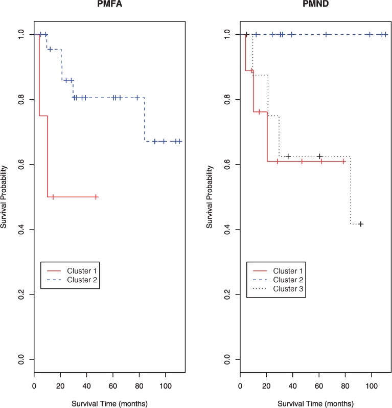
Survival curves for the clusters identified by PMFA and PMND for the lung cancer data.

Note that a preliminary variable screening can be helpful even for a method with the capability of variable selection: in addition to saving computing time with a simple univariate variable screening, it can improve predictive performance, as theoretically shown by Fan and Lv (2008). For example, when the top 450, rather than 300, genes were used in PMFA, there was a less significant survival difference between the two clusters detected from the test data: the log-rank test gave a P-value of only 0.145.

4 DISCUSSION

We have proposed a new model-based clustering method, a PMFAs, to model non-diagonal cluster-specific covariance matrices. PMFA generalizes the usual MFAs via regularization, which can effectively realize variable selection in clustering high-dimensional data, in addition to regularizing parameter estimates and its associated benefits. Simulation studies and a microarray gene expression data application have demonstrated the utility of the proposed method and its superior performance over MFA and penalized model-based clustering with a common diagonal covariance matrix. Although the current implementation of the EM algorithm for PMFA is straightforward, it is computationally demanding, especially with the choice of the tuning parameters by a grid search. More efficient algorithms and model selection criteria will be helpful. Other possible extensions of PMFA include the following. First, although we only considered the L₁ penalization of mean parameters, other penalties, such as a grouped penalty (Wang and Zhu, 2008; Xie et al., 2008a) as for the loading matrix parameters considered here, can be applied. Second, it is natural to consider using general covariance matrices in the mixture model. In Zhou et al. (2009), we embed an unconstrained covariance matrix estimation procedure in the EM algorithm. Although the use of an unconstrained covariance matrix is more flexible than the PMFA approach, it may lose efficiency if some latent variable-induced covariance assumption holds as in the PMFA approach; numerical comparisons are needed.

REFERENCES

- Baek J, McLachlan GJ. Mixtures of factor analyzers with common factor loadings for the clustering and visualisation of high-dimensional data. Isaac Newton Institute for Mathematical Sciences; 2008. Preprints. [Google Scholar]
- Baek J, et al. Mixtures of factor analyzers with common factor loadings: applications to the clustering and visualisation of high-dimensional data. To appear in IEEE Transactions on Pattern Analysis and Machine Intelligence. 2009 doi: 10.1109/TPAMI.2009.149. Available at: http://www.maths.uq.edu.au/∼gjm/bmf_pami09.pdf/ [DOI] [PubMed] [Google Scholar]
- Beer DG, et al. Gene-expression profiles predict survival of patients with lung adenocarcinoma. Nat. Med. 2002;8:816–824. doi: 10.1038/nm733. [DOI] [PubMed] [Google Scholar]
- Dempster AP, et al. Maximum likelihood from incomplete data via the EM algorithm (with discussion) J. R. Stat. Soc. Series B. 1977;39:1–38. [Google Scholar]
- Eisen M, et al. Cluster analysis and display of genome-wide expression patterns. Proc. Natl Acad. Sci. USA. 1998;95:14863–14868. doi: 10.1073/pnas.95.25.14863. [DOI] [PMC free article] [PubMed] [Google Scholar]
- Everitt BS. An Introduction to Latent Variable Models. London: Chapman and Hall; 1984. [Google Scholar]
- Fan J, Lv J. Sure independence screening for ultrahigh dimensional feature space (with discussion) J. R. Stat. Soc. Series B. 2008;70:849–911. doi: 10.1111/j.1467-9868.2008.00674.x. [DOI] [PMC free article] [PubMed] [Google Scholar]
- Fraley C, Raftery AE. Model-based clustering, discriminant analysis, and density estimation. J. Am. Stat. Assoc. 2002;97:611–631. [Google Scholar]
- Fraley C, Raftery AE. Model-based methods of classification: using the mclust software in chemometrics. J. Stat. Software. 2007;18 paper i06. Available at http://www.jstatsoft.org/v18/i06/ [Google Scholar]
- Ghahramani Z, Hinton GE. Technical Report CRG-TR-96-1. Toronto, Canada: Department of Computer Science, University of Toronto; 1997. The EM algorithm for mixtures of factor analyzers. M5S 1A4, 1997. [Google Scholar]
- Golub T, et al. Molecular classification of cancer: class discovery and class prediction by gene expression monitoring. Science. 1999;286:531–537. doi: 10.1126/science.286.5439.531. [DOI] [PubMed] [Google Scholar]
- Hinton GE, et al. Modeling the manifolds of images of handwritten digits. IEEE Trans. Neural Networks. 1997;8:65–74. doi: 10.1109/72.554192. [DOI] [PubMed] [Google Scholar]
- Huang JZ, et al. Covariance selection and estimation via penalised normal likelihood. Biometrika. 2006;93:85–98. [Google Scholar]
- Hubert L, Arabie P. Comparing partitions. J. Classif. 1985;2:193–218. [Google Scholar]
- McLachlan GJ, Peel D. Mixtures of factor analyzers. In: Langley P, editor. Proceedings of the Seventeenth International Conference on Machine Learning. San Francisco: Morgan Kaufmann; 2000. pp. 599–606. [Google Scholar]
- McLachlan GJ, et al. A mixture model-based approach to the clustering of microarray expression data. Bioinformatics. 2002;18:413–422. doi: 10.1093/bioinformatics/18.3.413. [DOI] [PubMed] [Google Scholar]
- McLachlan GJ, Peel D. Finite Mixture Model. New York: John Wiley & Sons, Inc.; 2002. [Google Scholar]
- McLachlan GJ, et al. Modeling high-dimensional data by mixtures of factor analyzers. Comput. Stat. Data Analysis. 2003;41:379–388. [Google Scholar]
- McLachlan GJ, et al. Extension of the mixture of factor analyzers model to incorporate the multivariate t-distribution. Comput. Stat. Data Analysis. 2007;51:5327–5338. [Google Scholar]
- Pan W, Shen X. Penalized model-based clustering with application to variable selection. J. Mach. Learn. Res. 2007;8:1145–1164. [Google Scholar]
- Raftery AE, Dean N. Variable selection for model-based clustering. J. Am. Stat. Assoc. 2006;101:168–178. [Google Scholar]
- Rand WM. Objective criteria for the evaluation of clustering methods. J. Am. Stat. Assoc. 1971;66:846–850. [Google Scholar]
- Thalamuthu A, et al. Evaluation and comparison of gene clustering methods in microarray analysis. Bioinformatics. 2006;22:2405–2412. doi: 10.1093/bioinformatics/btl406. [DOI] [PubMed] [Google Scholar]
- Wang S, Zhu J. Variable selection for model-based high-dimensional clustering and its application to microarray data. Biometrics. 2008;64:440–448. doi: 10.1111/j.1541-0420.2007.00922.x. [DOI] [PubMed] [Google Scholar]
- Xie B, et al. Variable selection in penalized model-based clustering via regularization on grouped parameters. Biometrics. 2008a;64:921–930. doi: 10.1111/j.1541-0420.2007.00955.x. [DOI] [PubMed] [Google Scholar]
- Xie B, et al. Penalized model-based clustering with cluster-specific diagonal covariances and grouped variables. Electron. J. Stat. 2008b;2:168–212. doi: 10.1214/08-EJS194. [DOI] [PMC free article] [PubMed] [Google Scholar]
- Yuan M, Lin Y. Model selection and estimation in regression with grouped variables. J. R. Stat. Soc. Series B. 2006;68:49–67. [Google Scholar]
- Yuan M, Lin Y. Model selection and estimation in the Gaussian graphical model. Biometrika. 2007;94:19–35. [Google Scholar]
- Zhou H, et al. Penalized model-based clustering with unconstrained covariance matrices. Electronic J. Stat. 2009;3:1473–1496. doi: 10.1214/09-EJS487. [DOI] [PMC free article] [PubMed] [Google Scholar]
Associated Data
This section collects any data citations, data availability statements, or supplementary materials included in this article.