

Abstract
The medial temporal lobe (MTL) is critical for declarative memory formation. Several theories of MTL function propose functional distinctions between the different structures of the MTL, namely the hippocampus and the surrounding cortical areas. Furthermore, computational models and electrophysiological studies in animals suggest distinctions between the subregions of the hippocampus itself. Standard fMRI resolution is not sufficiently fine to resolve activity on the scale of hippocampal subregions. Several approaches to scanning the MTL at high resolutions have been made, however there are limitations to these approaches, namely difficulty in conducting group‐level analyses. We demonstrate here techniques for scanning the MTL at high resolution and analyzing the high‐resolution fMRI data at the group level. To address the issue of cross‐participant alignment, we employ the ROI‐LDDMM alignment technique, which is demonstrated to result in smaller alignment errors when compared with several other common normalization techniques. Finally, we demonstrate that the pattern of activation obtained in the high‐resolution functional data is similar to that obtained at lower resolution, although the spatial extent is smaller and the percent signal change is greater. This difference in the pattern of activation may be due to less partial volume sampling in the high‐resolution data, resulting in more accentuated regions of activation. Hum Brain Mapp 2006. © 2006 Wiley‐Liss, Inc.
Keywords: high‐resolution fMRI, medial temporal lobe, hippocampus, memory
INTRODUCTION
The medial temporal lobe (MTL) is known to be critically involved in declarative memory [Scoville and Milner, 1957; Squire et al., 2004]. Several different classes of theories of MTL function have posited functional distinctions between the various MTL structures. For example, the hippocampal region, including the dentate gyrus (DG), CA fields (CA1, CA3) and subiculum (SUB), is posited to support relational [Eichenbaum et al., 1994], recollective [Yonelinas, 2002] or associative [Aggleton and Brown, 1999; Brown and Aggleton, 2001] processing, while the adjacent MTL cortical areas (entorhinal, perirhinal, and parahippocampal cortices) are thought to support single‐item [Aggleton and Brown, 1999; Brown and Aggleton, 2001] or familiarity [Yonelinas, 2002] processes. Furthermore, computational models of the hippocampus posit further functional specialization within the hippocampus itself [Marr, 1971; McClelland et al., 1995; O'Reilly and Rudy, 2001; Rolls et al., 2002]. For example, Marr [1971] described the CA3 as an autoassociative network capable of pattern completion, a process whereby a previously stored pattern of activity can be re‐instantiated given noisy or degraded cues. Subsequent models have ascribed pattern separation (a process whereby overlapping or similar patterns of activity are orthogonalized in a sparse representation) to the DG.
While electrophysiological [Lee et al., 2004a, b; Leutgeb et al., 2004] and animal lesion [Kesner et al., 2000] data support the predictions of the models of hippocampal function, there are relatively few data from noninvasive neuroimaging techniques in humans bearing on the models' predictions. One difficulty is the spatial resolution of standard fMRI is too coarse to resolve activity within sub‐regions of the hippocampus. Several approaches at scanning the MTL at high resolution have been made.
In one, high‐resolution functional data have been collected and anatomical‐defined regions of interest (ROIs) have been used to collapse all data from an anatomical region (e.g. CA1) into a single functional timecourse [Preston et al., 2005]. The primary advantage of this technique is also its primary disadvantage. By collapsing all voxels within a region, signal‐to‐noise is increased if the region is largely homogeneous in function. If multiple functions (multiple patterns of activity) are present, this approach suffers. In a second approach, cortical unfolding techniques have been applied to the spiral structure of the hippocampus and adjacent cortex [Zeineh et al., 2000, 2003]. This converts the three‐dimensional structures into two‐dimensional “flat maps.” Accurate cross‐participant alignment is substantially easier in a flat 2D space than in a 3D space. However, when used in the hippocampus, this technique places heavy demands on the unfolding process. In attempting to unfold the hippocampus' tight spiral structure, any small misalignment between structural and functional data or any voxels that straddle two adjacent regions can lead to mislocalization of activity or a splitting of a single region of activity into two. Thus activity in a single voxel may be attributed to both DG and CA1, for example.
We describe here a novel approach to collecting and analyzing high‐resolution fMRI data. While the specific structures under investigation are the MTL structures underlying declarative memory, the techniques described are equally well‐suited to investigation of other brain regions and processes. For purposes of comparison, and to validate the high‐resolution scanning technique, we use a behavioral paradigm here that has been demonstrated to activate the MTL in a reliable fashion [Flanery and Stark, submitted; Law et al., 2005].
METHOD
Participants
Twenty right‐handed participants (8 female) gave written informed consent before participating. Mean age was 25.1 (range 20–46). One participant's data was excluded from the functional analysis due to excessive motion between scans. Participants were recruited from the Johns Hopkins community and were paid for their participation.
Behavioral Method
The behavioral task was that used by Law et al. [Law et al., 2005] and Flanery and Stark [submitted]. This is a task that has been demonstrated to elicit robust activation of the MTL, and therefore served as a benchmark task in evaluating the scanning and analysis methods. The stimuli were randomly generated kaleidoscope images [Miyashita et al., 1991]. For 132 trials per scan run, participants were first shown a stimulus with four square outlines superimposed on it. Participants were given four response buttons and instructed that each stimulus was paired with one of the buttons, corresponding to the four boxes on the screen. Participants were instructed to guess which response goes with each stimulus and were told that they would receive feedback regarding their guess. Thus, participants learned through trial and error the correct paired associate to each of the stimuli. During each trial, the initial stimulus presentation lasted 500 ms, followed by a 700 ms wait period. Participants were cued to make a response following the wait period during the response period, which lasted 700 ms. Participants were given feedback for 800 ms (“yes” if their response was the correct button associated with that stimulus, “no” if they were incorrect, and “?” if they failed to make a response in the response window). Twenty‐four to forty‐eight hours prior to scanning, participants were trained on the task using a set of four “reference” stimuli that remained constant throughout the task. During scanning, participants were required to learn from four to eight new test stimuli at a time in addition to the four reference stimuli. As performance on individual test stimuli improved, they were replaced, thus keeping the overall level of performance relatively constant across the scan session. In addition to test and reference trials, 32 null trials were also randomly interspersed in each run [Dale, 1999]. The overall structure of null trials was the same as test or reference trials, however instead of a kaleidoscopic image as a stimulus, participants were shown a fixed, random visual static pattern. One of the response boxes was randomly assigned as the target on each trial and was set at a slightly greater opacity than the other three boxes. The difference between the opacity of the target and the other boxes was set to be one of the more difficult levels as determined by [Law et al., 2005, experiment 2].
fMRI Imaging Parameters
MRI data were collected on a Phillips 3T scanner (Best, The Netherlands) equipped with a SENSE (sensitivity encoding) head coil at the F. M. Kirby Research Center for Functional Brain Imaging at the Kennedy Krieger Institute (Baltimore, MD). A parallel imaging technique, SENSE, was used to acquire the data that significantly reduced acquisition time and distortion attributable to magnetic susceptibility [Pruessmann et al., 1999]. Functional echoplanar images were collected using a high‐speed echoplanar single‐shot pulse sequence with an acquisition matrix size of 64 × 64, an echo time of 30 ms, a flip angle of 70°, a SENSE factor of 2, and an in‐plane acquisition resolution of 1.5 × 1.5 mm2. This voxel size (1.5 × 1.5 × 1.5 mm3) was chosen based on the results of Hyde et al. [Hyde et al., 2001] who showed that this voxel size demonstrated the greatest functional signal‐to‐noise ratio when compared with other cubic voxel sizes. It is worth noting that this reduction in slice thickness will also have the benefit of reducing spatial distortion [Buxton, 2001]. In each run, a total of 264 volumes were acquired with a TR of 1.5 s. Each volume consisted of 19 oblique axial slices aligned to the long axis of the hippocampus and centered to include the hippocampus and the parahippocampal gyrus. Data acquisition began after the fourth image to allow for stabilization of the MR signal.
For anatomical localization and cross‐participant alignment, a series of structural scans were acquired. The first was a standard whole‐brain, three‐dimensional magnetization‐prepared rapid gradient echo (MP‐RAGE) pulse sequence (150 oblique axial slices, 1 × 1 × 1 mm3 voxels). In addition, between three and five high‐resolution (60 oblique axial slices, 0.75 × 0.75 × 0.75 mm3 voxels) MP‐RAGE scans were acquired, which were later averaged and aligned with the standard MP‐RAGE. The high‐resolution MP‐RAGE scans afforded a more detailed picture of the subregions of the hippocampus and were used in defining these subregions in the cross participant alignment analysis (see next section).
fMRI Data Analysis
Data analysis was carried out using the Analysis of Functional Neuroimages (AFNI) software [Cox, 1996]. Functional data and high‐resolution structural data were coregistered in three dimensions to the standard whole‐brain anatomical data (Figure 2). Functional data were also coregistered through time to reduce any effects of head motion. Time periods in which a significant motion event (>3 degrees of rotation or 2 mm of translation in any direction) occurred, plus and minus 1 TR, were eliminated from the analysis. Following the analyses of Law et al. [2005] and Flanery and Stark [submitted], we sorted test trials according to memory strength, as determined by their behavioral performance. Briefly, we used a logistic regression algorithm developed by Brown and colleagues [Smith and Brown, 2003; Smith et al., 2004] to convert the binary performance on each trial to an estimate of memory strength. The algorithm uses the behavioral performance to estimate the probability that the next trial will be correct. Thus, based on this probability, each trial was sorted into one of five memory strength bins.
Figure 2.

Functional to structural coregistration. A: An oblique axial slice from a high‐resolution MP‐RAGE (0.75 × 0.75 × 0.75 mm3 voxels). The slice is aligned with the primary axis of the hippocampus, outlined here in red. B: The same outline overlaid on the functional EPI data for the same subject.
Behavioral vectors were then developed which coded for memory strengths 1–5, reference trials, and first presentations (the first time in the experiment a given stimulus was seen). These vectors were used in an analysis using a deconvolution approach based on multiple linear regression (3dDeconvolve; http://afni.nimh.nih.gov/pub/dist/doc/manuals/3dDeconvolve.pdf). The resultant fit coefficients (β coefficients) represent activity versus baseline for a given time point and trial type in a voxel. The sum of the fit coefficients over the expected hemodynamic response (∼3–12 s after trial onset) was taken as the estimate of the model of the response to each trial type (relative to the null‐task baseline), which was converted to percent signal change.
Cross Participant Alignment
The cross participant alignment used an example of the region of interest alignment (ROI‐AL) approach developed by our laboratory [Stark and Okado, 2003]. This approach uses an objective function that maximizes the overlap of 3D segmented ROI labels (i.e., hippocampus atop hippocampus, perirhinal cortex atop perirhinal cortex, etc). In particular, the technique used here extends the version of ROI‐AL that employs large deformation diffeomorphic metric mapping (ROI‐LDDMM) [Miller et al., 2005] to map between an individual parpticipant's 3D ROI segmentation and a 3D template segmentation of the MTL. LDDMM creates a 3D vector field that smoothly transforms images between coordinate systems so that connected sets remain connected, disjoint sets remain disjoint, and submanifold structures are preserved. This preservation is particularly important for averaging functional data where the bijective property of the maps ensures that artifacts because of superposition of functional data from neighboring regions are avoided.
The alignment of the structural and functional data proceeded in several steps. First, all participants' anatomical and functional scans were normalized to the Talairach atlas [Talairach and Tournoux, 1988] using AFNI. This was done to provide a rough initial alignment and remove large spatial shifts between subjects, thus improving the potential performance of ROI‐LDDMM. Anatomical regions of interest were fully segmented in 3D on the Talairach transformed standard (1 mm3) MP‐RAGE images for the temporal polar, entorhinal, and perirhinal cotices according the landmarks described by Insausti et al.[1998]. The parahippocampal cortex was defined bilaterally as the portion of the parahippocampal gyrus caudal to the perirhinal cortex and rostral to the splenium of the corpus callosum, as in our previous research [Kirwan and Stark, 2004; Law et al., 2005; Stark and Okado, 2003].
Extending our previous techniques, the subfields of the hippocampus were also defined bilaterally. The subfield of the hippocampus were defined as the DG/CA3 (dentate gyrus and CA3 field), CA1, and SUB (subiculum) [Csernansky et al., 2005; Wang et al., 2003] following the atlas of Duvernoy [1998] using the high‐resolution (0.75 mm3) MP‐RAGE (see Fig. 1B). Duvernoy [1998] describes eight coronal slices along the anterior–posterior axis of the hippocampus. Representative slices in each hippocampus that best (closest) resembled the slices described were chosen and segmented according to the atlas description. The segmentation then proceeded from these slices in both directions slice by slice to ensure a smooth transition between the slices.
Figure 1.
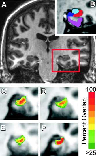
MTL segmentation. A: A coronal section from a standard (1 mm3) MP‐RAGE. The red box indicates the area enlarged in B–F. B: The same coronal slice with the anatomical regions CA1 (red), CA3/DG (light blue), Subiculum (dark blue), and parahippocampal cortex (purple) overlayed. Not shown are entorhinal, perirhinal, and temporopolar cortex. Average alignment of 20 subjects' CA1 region after alignment with C: FSL, D: SPM, E: Talairach, and F: ROI‐LDDMM. Red areas indicate 100% overlap, while green indicates <25% overlap between subjects.
A model for the ROI‐LDDMM transformation calculations was then constructed by first choosing a single participant (number 2) to serve as the initial model for the transformation calculation for all the other participants. Once each participant's set of ROIs had been warped to the subject model, a central tendency was determined by taking the mode of all 20 participants' transformed ROI labels. This central tendency (the modal model) then served as the model for subsequent ROI‐LDDMM transformations as each individual subject's MTL ROIs was warped with ROI‐LDDMM onto the model.
Percent signal change maps were first transformed to Talairach space keeping the same (1.5 mm3) resolution. The maps were then blurred with a 3‐mm full‐width at half maximum (FWHM) Gaussian kernel that respected the anatomical boundaries defined for each participant's MTL. In order to minimize the loss of spatial resolution due to blurring but at the same time account for any residual inter‐subject functional variability, we chose a small (3 mm) kernel and constrained the blur such that the statistical maps were blurred within the anatomically defined ROIs. This approach results in a small loss of spatial resolution within an individual ROI, but by cutting off the blur at the anatomical boundaries defined within the MTL, the localization of activations between regions of the MTL does not suffer from this loss. Finally, the transformation matrix calculated for each subject in the ROI‐LDDMM process was applied to the statistical maps.
To validate the alignment technique and for comparison, the ROIs were aligned using several other methods, including FLIRT [Jenkinson et al., 2002] in the FSL analysis package (http://www.fmrib.ox.ac.uk/fsl/index.html), SPM2 (http://www.fil.ion.ucl.ac.uk/spm/), and ROI‐LDDMM using the same 10 ROI model (bilateral temporal polar, perirhinal, entorhinal, parahippocampal cortices and the hippocampus without subfield segmentation) as Miller et al. [2005]. For each alignment technique, the datasets were first normalized to Talairach space using AFNI. For FSL and SPM alignment, the segmented ROIs were transferred from AFNI to ANALYZE format and normalized using nearest neighbor interpolation. All other normalization parameters were left at the default values for the respective programs. The resulting aligned ROIs from each alignment technique were then blurred using Gaussian kernel with σ = 0.5 mm. This was done in order to reduce the error originating from misalignment on the edges of the ROIs, effectively assigning a greater weight to the interior of the ROIs when calculating the error metric.
The error metric was calculated using MATLAB (The MathWorks, Natik, MA) by taking the absolute difference between a given transformed data set and a target dataset and then normalizing by dividing by the volume of the unblurred target. This was calculated for each of the respective alignment techniques. In order to produce an unbiased estimate of this error, each subject in turn served as the target against which all other subjects were compared. The mean of these scores was taken as the error metric for each of the alignment techniques.
Low‐Resolution Data
To validate the present method of high‐resolution fMRI scanning, we compared our results with those obtained by Law et al. [2005] and Flanery and Stark [submitted] using the same behavioral paradigm and an equal number of participants (19). Participants and data analysis methods are as described in Law et al. [2005], with the exception that fMRI data were converted to percent signal change from the common baseline task in order to facilitate direct comparison between the two experimental conditions.
RESULTS
Behavioral Performance
Behavioral performance was similar to that observed by Law et al. [2005]. Across participants, the mean number of new stimuli learned per scan run was 6.20 (SEM 0.38; range 3–8.8).
Cross‐Participant Alignment
Table I presents the mean alignment error for each of the anatomically defined ROIs after alignment with each of the alignment techniques. A two‐way ANOVA revealed significant main effects of ROI and alignment method, as well as a significant ROI by alignment method interaction (all P < 0.001). Figure 3 presents the mean alignment error for the hippocampus averaged across all subjects for each of the registration techniques with each subject serving as target compared with all the other subjects. A one‐way ANOVA revealed a significant effect of alignment technique [F (4,76) = 195.24, P < 0.00001]. Post hoc t‐tests revealed that alignment with LDDMM to the fully defined model (including hippocampal subregions) resulted in significantly lower errors than the other techniques [all t(19) > 9, P < 0.001]. Error following normalization with FSL and SPM2 were similar to each other (t < 1) and error following the AFNI Talairach transformation was somewhat greater than FSL or SPM2 (all P < 0.002).
Table I.
Mean error score (SEM) by medial temporal lobe anatomical region of interest for each alignment technique
| Anatomical ROI | Alignment technique | |||||
|---|---|---|---|---|---|---|
| Talairach | FSL | SPM | LDDMM1 | LDDMM2 | ||
| CA1 | R | 1.31 (0.09) | 1.19 (0.08) | 1.21 (0.08) | 0.66 (0.04) | 0.50 (0.03) |
| L | 1.31 (0.10) | 1.24 (0.09) | 1.25 (0.09) | 0.67 (0.04) | 0.51 (0.03) | |
| CA3 | R | 1.44 (0.11) | 1.32 (0.19) | 1.29 (0.09) | 0.71 (0.05) | 0.59 (0.04) |
| L | 1.48 (0.12) | 1.41 (0.10) | 1.45 (0.11) | 0.74 (0.05) | 0.64 (0.04) | |
| Subiculum | R | 1.47 (0.11) | 1.36 (0.10) | 1.40 (0.10) | 0.79 (0.06) | 0.75 (0.05) |
| L | 1.50 (0.11) | 1.48 (0.11) | 1.51 (0.11) | 0.82 (0.06) | 0.87 (0.05) | |
| Temporalpolar Ctx. | R | 1.16 (0.09) | 1.18 (0.10) | 1.09 (0.08) | 0.53 (0.05) | 0.34 (0.02) |
| L | 1.24 (0.09) | 1.27 (0.09) | 1.17 (0.08) | 0.55 (0.05) | 0.35 (0.02) | |
| Perirhinal Ctx. | R | 1.36 (0.11) | 1.25 (0.09) | 1.25 (0.10) | 0.70 (0.05) | 0.76 (0.05) |
| L | 1.28 (0.10) | 1.17 (0.08) | 1.17 (0.08) | 0.67 (0.05) | 0.78 (0.05) | |
| Entorhinal Ctx. | R | 1.33 (0.09) | 1.36 (0.09) | 1.27 (0.09) | 0.72 (0.05) | 0.65 (0.04) |
| L | 1.31 (0.08) | 1.32 (0.09) | 1.25 (0.08) | 0.72 (0.05) | 0.61 (0.04) | |
| Parahippocampal Ctx. | R | 1.18 (0.09) | 1.06 (0.08) | 1.03 (0.08) | 0.69 (0.05) | 0.75 (0.07) |
| L | 1.34 (0.14) | 1.21 (0.12) | 1.25 (0.12) | 0.70 (0.05) | 0.78 (0.07) | |
Figure 3.
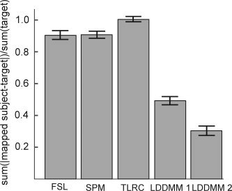
Cross‐participant hippocampal alignment error. Error rates for each of the alignment techniques were defined as the absolute difference between each mapped subject and every other subject as a target subject, normalized by the target subject volume (see text). LDDMM 1 indicates ROI‐LDDMM alignment to a model that lacked segmentation of the hippocampal subregions. The model in LDDMM 2 included the subregional segmentation.
Functional Data Replication
Using the same behavioral paradigm as in the present study, Law et al. [2005] and Flanery and Stark [submitted] found that activity in the MTL increased in a linear fashion from memory strength 1 through memory strength 5 and the reference condition. The greatest activity difference between conditions was between memory strengths 1 and 5. We therefore performed t‐tests contrasting memory strengths 1 and 5 for the low‐ and high‐resolution data. For both datasets, we created functionally defined regions of interest (ROIs) by setting a voxel‐wise threshold of P = 0.03 for the t‐test and a spatial extent threshold resulting in an overall probability of P = 0.05 as determined by Monte Carlo simulations (AFNI's AlphaSim program) for the MTL volume (29,578 mm3 and 29,484 mm3 for the low and high‐resolution data respectively). Finally, the ROIs were masked to exclude non‐MTL voxels by blurring the model MTL used for the LDDMM alignment for the respective datasets with a 3‐mm FWHM Gaussian blur. Thus, what are reported below as significant regions of activation have a P‐value of less than 0.05.
In the low‐resolution dataset, this analysis yields two large ROIs encompassing the entire rostral‐caudal extent of the hippocampus bilaterally (Fig. 4A). Consistent with the findings of [Hyde et al., 2001], the activations in the high‐resolution dataset are much smaller than in the low‐resolution data (e.g., 243 mm3 vs. 906 mm3 in the right hippocampus). In the high‐resolution MTL data, there are two significant regions of activation in the left hippocampus, and a third in the anterior right hippocampus (Fig. 3A). To localize the regions of activation within the MTL, the percent overlap between the functionally‐defined ROIs and the modal model was calculated. The anterior left hippocampal ROI was 32 voxels, 6.25% of which overlapped with CA3. The rest fell just outside the area defined as MTL. In the posterior left hippocampal activation, 40.91% fell within CA3, while 59.09% fell in CA1. On the right, the hippocampal activation fell within CA3 (51.4%), CA1 (11.11%), and subiculum (2.78%). The remaining 34.72% fell outside regions defined as MTL in the model. In both hemispheres, the activity detected in the low and high‐resolution datasets overlap considerably.
Figure 4.
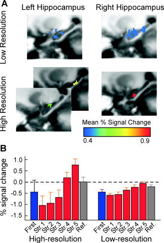
A: Significant regions of functional activation in the low‐ and high‐resolution datasets. Region of interest color corresponds to the mean percent signal change. B: Example pattern of activation in the left hippocampus (anterior region in the high‐resolution dataset). Memory strengths 1–5 (i.e. Str1–5) were estimated from the binary performance on each trial (see text). High and low‐resolution functional data show a similar pattern of activation with greater percent signal change seen in the smaller voxels.
We predicted based on the results of Hyde et al. [2001] that the percent signal change would be greater at high resolution than at low resolution. To test this hypothesis, we indexed signal change related to learning by contrasting activity between memory strengths 1 and 5 for the similar regions in the high versus low resolution data sets (Fig. 3B). The mean percent signal change in the left hippocampal ROI was significantly greater in the high‐resolution dataset in both the anterior ROI [mean = 1.80, t(36) = 3.17, P < 0.01] and the posterior ROI [mean = 1.37, t(36) = 2.51, P < 0.05] separately compared with the low resolution ROI in the left hippocampus (mean = 0.53). In the right hippocampus, the mean percent signal change was again greater in the high‐resolution dataset compared with the low‐resolution data, with a mean of 1.48 and 0.55 in the high‐ and low‐resolution datasets, respectively [t(36) = 3.69, P < 0.001]. Thus the high‐resolution data replicates the low‐resolution data in terms of the overall pattern of activation, however the activations observed were more specific and showed a greater percent signal change.
DISCUSSION
Theories of MTL function in declarative memory commonly posit a functional distinction between the hippocampus and the adjacent cortical areas. Furthermore, electrophysiological data and computational models of the hippocampus suggest functional distinctions within subregions of the hippocampus. However, there are several challenges to using fMRI to resolve activity within the different structures of the MTL, and especially within subregions of the hippocampus. The first challenge is that the standard fMRI resolution is too coarse to localize activity at the level required. A second challenge is that cross‐participant alignment of the functional data must be precise in order to take advantage of a group‐level analysis. This experiment used a combination of approaches to address these issues.
First, we demonstrated that the ROI‐LDDMM alignment technique is reliably more precise at aligning the hippocampus in a group of subjects than other commonly used normalization techniques. When testing hypotheses about specific brain regions, such as the MTL, it is advantageous to restrict investigation and analysis to that brain region. We employ this approach by only collecting fMRI data from the MTL and basing the alignment on anatomical definitions of the MTL structures themselves (the ROI‐AL approach, instantiated here as ROI‐LDDMM). Presumably, other automated normalization procedures, such as those employed by FSL and SPM2, would also benefit from restricting their venue to a local area (such as the MTL). This is a possible avenue for further research, but while such an approach will likely improve these basic techniques, they will likely not achieve the accuracy achieved here with this alone. One strength of the ROI‐AL approach is to restrict the alignment to a smaller volume, but a second is to use an error metric during alignment that is based on the overlap of 3D segmentations of regions. Typical approaches use the difference in greyscale intensity across images and can easily align one participant's entorhinal cortex (grey matter) atop another participant's perirhinal cortex (nearby grey matter). Finally, the LDDMM alignment algorithm provides greater flexibility in alignment and higher accuracy than other algorithms commonly used in neuroimaging research [Beg et al., 2005]. This increase in accuracy also increases the confidence with which a given activation may be localized to specific structures, such as the subregions of the hippocampus both by the overall reduction in alignment error and by the explicit use of 3D anatomical segmentations of the specific structures. This latter point allows one to interrogate a voxel's location and anatomical label (e.g. right CA1 or left perirhinal cortex) both in the template (representing some central tendency across individual brains) and in each individual's brain segmentation.
We also demonstrated that the high‐resolution functional data replicates the memory strength effects observed at lower resolution. Furthermore, the pattern of activation observed in the high‐resolution data had a similar spatial distribution (bilateral hippocampus), but covered a much smaller area. This may be due to less partial sampling of activated regions in the high‐resolution data. This is supported by the fact that we observed significantly greater percent signal change in the high‐resolution ROIs. In conclusion, it appears that we can successfully perform high‐resolution fMRI in the MTL.
In conclusion, we present here a combination of high‐resolution fMRI and cross‐participant alignment techniques that allow us to resolve fine‐scale activity within the MTL using a group‐level analysis. Although the current approach does not allow us to measure activity in other brain regions outside the MTL, the techniques employed here are generalizable and not restricted to use with just the MTL. These same techniques can be applied to any structure or collection of structures that can be anatomically segmented.
Acknowledgements
The authors thank J.R. Law and M.A. Flanery for their gracious help in data collection and analysis. M.I. Miller's work was supported by National Institute of Mental Health Grant 5 R01 EB00975‐01 and National Institute of Health Grant 1 P41 RR15241‐01A1.
REFERENCES
- Aggleton JP, Brown MW ( 1999): Episodic memory, amnesia, and the hippocampal‐thalamic axis. Behav Brain Sci 22: 425–444. [PubMed] [Google Scholar]
- Beg MF, Miller MI, Trouve A, Younes L ( 2005): Computing metrics via geodesics on flows of diffeomorphisms. Int J Comput Vis 61: 139–157. [Google Scholar]
- Brown MW, Aggleton JP ( 2001): Recognition memory: What are the roles of the perirhinal cortex and hippocampus? Nat Rev Neurosci 2: 51–61. [DOI] [PubMed] [Google Scholar]
- Buxton RB ( 2001): Introduction to Functional Magnetic Resonance Imaging: Principles and Techniques. Cambridge University Press. [Google Scholar]
- Cox RW ( 1996): AFNI: Software for analysis and visualization of functional magnetic resonance neuroimages. Comput Biomed Res 29: 162,163. [DOI] [PubMed] [Google Scholar]
- Csernansky JG, Wang L, Swank J, Miller JP, Gado M, McKeel D, Miller MI, Morris JC ( 2005): Preclinical detection of Alzheimer's disease: Hippocampal shape and volume predict dementia onset in the elderly. Neuroimage 25: 783–792. [DOI] [PubMed] [Google Scholar]
- Dale AM ( 1999): Optimal experimental design for event‐related fMRI. Hum Brain Mapp 8: 109–114. [DOI] [PMC free article] [PubMed] [Google Scholar]
- Duvernoy H ( 1998): The Human Hippocampus. New York: Springer‐Verlag. [Google Scholar]
- Eichenbaum H, Otto T, Cohen NJ ( 1994): Two component functions of the hippocampal memory system. Behav Brain Sci 17: 449–517. [Google Scholar]
- Flanery MA, Stark CEL: When negative is not negative: Activation in medial temporal lobe can vary with baseline task difficulty and trial repetition (submitted for publication).
- Hyde JS, Biswal BB, Jesmaniwicz A ( 2001): High‐resolution fMRI using multislice partial k‐space GR‐EPI with cubic voxels. Magn Reson Med 46: 114–125. [DOI] [PubMed] [Google Scholar]
- Insausti R, Juottonen K, Soininen H, Insausti AM, Partanen K, Vainio P, Laakso MP, Pitkanen A ( 1998): MR volumetric analysis of the human entorhinal, perirhinal, and temporopolar cortices. Am J Neuroradiol 19: 659–671. [PMC free article] [PubMed] [Google Scholar]
- Jenkinson M, Bannister PR, Brandy JM, Smith SM ( 2002): Improved optimisation for the robust and accurate linear registration and motion correction of brain images. Neuroimage 17: 825–841. [DOI] [PubMed] [Google Scholar]
- Kesner RP, Gilbert PE, Wallenstein GV ( 2000): Testing neural network models of memory with behavioral experiments. Curr Opin Neurobiol 10: 260–265. [DOI] [PubMed] [Google Scholar]
- Kirwan CB, Stark CEL ( 2004): Medial temporal lobe activation in a cued recall fmri paradigm. Cognitive Neuroscience Society Annual Meeting Program, San Francisco, CA. Program No. B103.
- Law JR, Flanery MA, Wirth S, Yanike M, Smith AC, Frank LM, Suzuki WA, Brown EN, Stark CEL ( 2005): Functional magnetic resonance imaging activity during the gradual acquisition and expression of paired‐associate memory. J Neurosci 25: 5720–5729. [DOI] [PMC free article] [PubMed] [Google Scholar]
- Lee I, Rao G, Knierim JJ ( 2004a): A double dissociation between hippocampal subfields: Differential time course of CA3 and CA1 place cells for processing changed environments. Neuron 42: 803–815. [DOI] [PubMed] [Google Scholar]
- Lee I, Yoganarasimha D, Rao G, Knierim JJ ( 2004b): Comparison of population coherence of place cells in hippocampal subfields CA1 and CA3. Nature 430: 456–459. [DOI] [PubMed] [Google Scholar]
- Leutgeb S, Leutgeb JK, Treves A, Moser M, Moser EI ( 2004): Distinct ensemble codes in hippocampal areas CA3 and CA1. Science 305: 1295–1298. [DOI] [PubMed] [Google Scholar]
- Marr D ( 1971): Simple memory: A theory for archicortex. Philos Trans R Soc Lond B Biol Sci 262: 23–81. [DOI] [PubMed] [Google Scholar]
- McClelland JL, McNaughton BL, O'Reilly RC ( 1995): Why there are complementary learning systems in the hippocampus and neocortex: Insights from the successes and failures of connectionist models of learning and memory. Psychol Rev 102: 419–457. [DOI] [PubMed] [Google Scholar]
- Miller MI, Beg MF, Ceritoglu C, Stark C ( 2005): Increasing the power of functional maps of the medial temporal lobe by using large deformation diffeomorphic metric mapping. Proc Natl Acad Sci USA 102: 9685–9690. [DOI] [PMC free article] [PubMed] [Google Scholar]
- Miyashita Y, Higuchi S, Saki K, Masui N ( 1991): Generation of fractal patterns for probing the visual memory. Neurosci Res 12: 307–311. [DOI] [PubMed] [Google Scholar]
- O'Reilly RC, Rudy JW ( 2001): Conjunctive representations in learning and memory: Principles of cortical and hippocampal function. Psychol Rev 108: 311–345. [DOI] [PubMed] [Google Scholar]
- Preston AR, Gaare ME, Wagner AD ( 2005): High‐resolution fMRI of stimulus‐specific novelty encoding and subsequent memory responses in human medial temporal lobe. Washington,DC: Society for Neuroscience. Report nr 353.4. [Google Scholar]
- Pruessmann K, Weiger M, Scheidegger N, Boesiger P ( 1999): SENSE: Sensitivity encoding for fast MRI. Magn Reson Med 42: 952–962. [PubMed] [Google Scholar]
- Rolls ET, Stringer SM, Trappenberg TP ( 2002): A unified model of spatial and episodic memory. Proc R Soc Lond B Biol Sci 269: 1087–1093. [DOI] [PMC free article] [PubMed] [Google Scholar]
- Scoville WB, Milner B ( 1957): Loss of recent memory after bilateral hippocampal lesions. J Neurol Neurosurg Psychiatry 20: 11–21. [DOI] [PMC free article] [PubMed] [Google Scholar]
- Smith AC, Brown EN ( 2003): Estimating a state‐space model from point process observations. Neural Comput 15: 965–991. [DOI] [PubMed] [Google Scholar]
- Smith AC, Frank LM, Wirth S, Yanike M, Hu D, Kubota Y, Graybiel AM, Suzuki WA, Brown EN ( 2004): Dynamic analysis of learning in behavioral experiments. J Neurosci 24: 447–461. [DOI] [PMC free article] [PubMed] [Google Scholar]
- Squire LR, Stark CEL, Clark RE ( 2004): The medial temporal lobe. Annu Rev Neurosci 27: 279–306. [DOI] [PubMed] [Google Scholar]
- Stark CEL, Okado Y ( 2003): Making memories without trying: Medial temporal lobe activity associated with incidental memory formation during recognition. J Neurosci 23: 6748–6753. [DOI] [PMC free article] [PubMed] [Google Scholar]
- Talairach J, Tournoux P ( 1988): A Co‐Planar Stereotaxic Atlas of the Human Brain. New York: Thieme Medical. [Google Scholar]
- Wang L, Swank JS, Glick IE, Gado MH, Miller MI, Morris JC, Csernansky JG ( 2003): Changes in hippocampal volume and shape across time distinguish dementia of the Alzheimer type from healthy aging. Neuroimage 20: 667–682. [DOI] [PubMed] [Google Scholar]
- Yonelinas AP ( 2002): The nature of recollection and familiarity: A review of 30 years of research. J Mem Lang 46: 441–517. [Google Scholar]
- Zeineh MM, Engel SA, Bookheimer SY ( 2000): Application of cortical unfolding techniques to functional MRI of the human hippocampal region. Neuroimage 11: 668–683. [DOI] [PubMed] [Google Scholar]
- Zeineh MM, Engel SA, Thompson PM, Bookheimer SY ( 2003): Dynamics of the hippocampus during encoding and retrieval of face‐name pairs. Science 299: 577–580. [DOI] [PubMed] [Google Scholar]