Perceptual Discrimination In Static and Dynamic Noise: The Temporal Relation Between Perceptual Encoding and Decision-making

Abstract

We report nine new experiments and reanalyze three published experiments that investigate factors affecting the time course of perceptual processing and its effects on subsequent decision making. Stimuli in letter discrimination and brightness discrimination tasks were degraded with static and dynamic noise. The onset and the time course of decision making were quantified by fitting the data with the diffusion model. Dynamic noise and, to a lesser extent, static noise, produced large shifts in the leading edge of the RT distribution in letter discrimination but had little effect in brightness discrimination. We interpret these shifts as changes in the onset of decision making. The different pattern of shifts in letter discrimination and brightness discrimination implies that decision making in the two tasks was affected differently by noise. The changes in RT distributions found with letter stimuli are inconsistent with the hypothesis that noise increases RTs to letter stimuli simply by reducing the rate at which evidence accumulates in the decision process. Instead, they imply that noise also delays the time at which evidence accumulation begins. The delay is shown not to be the result of strategic processes or the result of using different stimuli in different tasks. Our results imply, rather, that the onset of evidence accumulation in the decision process is time-locked to the perceptual encoding of the stimulus features needed to do the task. Two mechanisms that could produce this time-locking are described.

When a new stimulus first appears in the visual field, how do we process it and make a decision about its identity? A partial answer to this question can be found in the literature on stage models of information processing (Sternberg, 1969). The answer, which has its origins in the work of Donders (1969) a century earlier, holds that information processing consists of a sequence of mental operations, or processing stages, which transform stimulus energy arriving at the sensory receptors into overt responses. To make a decision about a stimulus we must first encode it perceptually, then match the perceptual representation against knowledge stored in memory, and then select and execute an appropriate behavioral response.

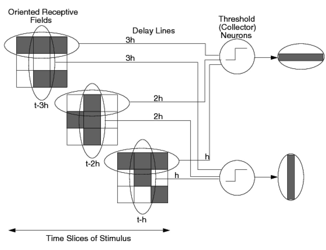
The process of matching stimulus information against stored knowledge to make a decision is well described by sequential-sampling models, like the diffusion model (Ratcliff, 1978; Ratcliff & Smith, 2004). These models hold that decisions are made by accumulating noisy evidence over time until a criterion quantity of evidence for a response is obtained. The evidence can be thought of as the goodness-of-match between the encoded stimulus and the memory representation of the response alternatives for the task. This view of decision making implies that perceptual processes and decision processes must be closely coupled, both in time, and in their underlying neural mechanisms. Before the process of evidence accumulation can begin, an encoded representation of the stimulus must be formed. Some mechanism must then initiate the process of evidence accumulation by the decision mechanism; that is, something must tell the decision mechanism when to "turn on."

The theoretical need for such a mechanism follows from the view that decisions are made by accumulating noisy evidence over time. Without such a mechanism, in the absence of a stimulus, a free running decision process will simply accumulate noise. This would lead to highly degraded performance and a preponderance of fast errors, as was first recognized by Laming (1968). The fact that this does not occur implies that the process of noisy evidence accumulation is initiated by the presentation and encoding of the stimulus. This means either that there is no noise in the system prior to stimulus presentation or that the noise that is present is not accumulated. If we think of the evidence as arising from a process of matching a stimulus to memory, these alternatives lead to two possible ways in which decision making could be initiated. The first assumes the noise in the matching process arises as a result of stimulus encoding. Prior to stimulus presentation the mean and variance of the matching process are both zero; there is no evidence accumulation because there is nothing to accumulate. The second possibility is that some more global process signals when formation of a perceptual representation of a stimulus is complete. Noise present in the system prior to this signal is not accumulated because the process of accumulation only begins after this signal is received. In addition to these possibilities, the onset of evidence accumulation may either be abrupt or it may develop slowly over time. Abrupt onsets are assumed by Ratcliff’s (1978) diffusion model and by most other sequential-sampling models in the literature. Progressive onsets are assumed in the visual short-term memory (VSTM) model of Smith and Ratcliff (2009). This latter model is a form of noisy cascade model, which has features in common with the cascade model of McClelland (1979). It differs from McClelland’s model, however, in that it assumes within-trial noise.

In this article, we investigate the temporal relationship between perception and decision making. The experiments we report identify factors that affect the time course of perceptual processing and its effects on subsequent decision making. Our interest in identifying these factors was to try to ascertain how and when the process of evidence accumulation is initiated. We find there are situations in which the diffusion model, in its current simplest form, fails to provide a satisfactory account of experimental data. This failure is highly illuminating as it points to a need to develop system models in which perceptual processes, decision processes, and the relationship between them are all specified.

Our approach to identifying the components of processing involved in making a decision about a stimulus differs from other methods in the literature, in that we use the diffusion model as a tool to perform process decomposition. Specifically, we use the diffusion model to identify the component of the response time (RT) distribution attributable to decision making and the component attributable to other processes. Our process modeling approach differs from property testing approaches to RT analysis, like the additive factors method of Sternberg (1969), the cascade model of McClelland (1979), or the critical path analysis of Schweickert (1978). The goal of these approaches is to draw strong inferences about the stage structure of performance in a task from relatively weak assumptions about the nature of the stages themselves.

We believe that process modeling has a number of advantages over property testing as a way to investigate the questions we are concerned with here. The first is that the diffusion model provides an account of performance at the level of the RT distributions for correct responses and errors simultaneously. It also provides an account of the relationship between RT and accuracy and how they covary as a function of task difficulty and experimental instructions. The weak assumptions made by property testing approaches are insufficient to predict performance at this level of detail. A second limitation of property testing approaches is that, while they seek to draw inferences based on weak assumptions about the underlying stages, the inferences nevertheless remain model-dependent. Changes in the assumptions about the general properties of stages leads to changes in the predicted patterns of additivity and interaction between them. Because the predictions from the property testing approach are not in fact model free, our preference is instead to adopt a strong process-modeling approach that can predict RT and accuracy in detail.

We also believe the diffusion model approach to process decomposition is preferable to methods that use atheoretical distributional models, like the ex-Gaussian (Hohle, 1965; Ratcliff & Murdock, 1976), or the Weibull (Rouder, Tuerlinckx, Speckman, Lu, & Gomez, 2008). The parameters of such models characterize features of the RT distribution, such as its location on the time axis, its dispersion, and its shape. In contrast, the parameters of models like the diffusion model characterize the underlying psychological process, rather than the distribution itself. In the case of the diffusion model, the parameters specify the rate at which evidence is accumulated, the amount of evidence needed for a decision, and the time for processes other than decision making. Because these parameters all have meaningful psychological interpretations, they can provide insight into the processes underlying performance. The parameters of atheoretical models, which are purely descriptive, do not provide insights of this kind. In this article, we investigate the time required to make a perceptual decision and the time at which the decision process begins. This question is addressed most directly by using a model of the decision process to decompose the RT distribution.

To date, diffusion models have been very successful in accounting for performance in a wide variety of experimental tasks in which speeded simple decisions are made. These include low-level perceptual tasks, such as simple reaction time, brightness discrimination, and signal detection (Ratcliff, 2002; Ratcliff & Rouder, 1998; Ratcliff, Van Zandt & McKoon, 1999; Smith, 1995; Smith, Ratcliff, & Wolfgang, 2004), and higher-level cognitive tasks such as lexical decisions and recognition memory (Ratcliff, 1978; Ratcliff, Thapar & McKoon, 2004; Ratcliff, Gomez, & McKoon, 2004; Ratcliff & Smith, 2004). The models have accounted for RT distributions for correct responses and errors, and the way in which the distributions change as a function of stimulus discriminability, response bias, speed-accuracy instructions, and other experimental variables. None of the experimental paradigms investigated to date has shown systematic discrepancies between theory and data. This has led some researchers to question whether diffusion models can account for any patterns of experimental data whatsoever.

To show that is not the case, Ratcliff (2002) described several patterns of empirical data that would falsify his diffusion model (Ratcliff, 1978). Among them was one in which the mean and the leading edge of the distribution changed by a similar amount with changes in stimulus discriminability. If stimulus discriminability affects only the rate of evidence accumulation -- represented in the diffusion model as a change in drift rate -- the model predicts that the leading edge of the RT distribution will change very little relative to the rest of the distribution (i.e., its median or its tail).

In this article, we present data from a letter discrimination task and a brightness discrimination task, in which stimuli are presented in static or dynamic noise. In the letter discrimination task, a white letter is presented on a black background. The letter is degraded by randomly reversing the contrast polarity of some proportion of the pixels in both the letter and the background. That is, some proportion of the letter pixels are changed to black while the same proportion of the background pixels are changed to white. When this proportion equals 50%, the display becomes a homogeneous, random array of black and white pixels, and the letter is no longer visible. In the dynamic version of the task, a different random sample of pixels is presented every 10 or 16.67 ms, one per frame of the video display.

Phenomenologically, when the proportion of inverted pixels is high (e.g., 45%), the stimulus letter seems to gradually emerge from the noise, whereas when the proportion is low (e.g., 15%), the letter seems to become perceptually available almost immediately. The critical finding is that the leading edge of the RT distribution in this task increases by 50–100 ms more than is predicted by the diffusion model as discriminability is changed from its highest to its lowest level. These predictions were obtained by making the usual assumption that only the rate of evidence accumulation (drift rate) changes with stimulus discriminability. Later we show that the change in the leading edge can be captured by relaxing this assumption. Although we use the Ratcliff (1978) diffusion model to fit our data, other models that use racing diffusion processes (Ratcliff, 2006; Ratcliff & Smith, 2004; Smith, 2000; Usher & McClelland, 2001) face a similar problem. These models cannot produce a large change in the leading edge of the RT distribution with only a change in the drift rate. This presents a significant theoretical challenge for models of perceptual decision making.

In the brightness discrimination task, the stimulus consists of a rectangular array of black and white pixels. Each pixel was randomly and independently set to black or white with some probability that determined the overall brightness of the array. Subjects are required to judge whether the array contains more black or white pixels and to make a "dark" or "light" response. In the experiments described here, we consider a dynamic version of this task, in which a different random sample of black and white pixels is presented every 10 ms, just as in the letter discrimination task. Unlike letter discrimination, this paradigm produces RT distributions in which the leading edge of the RT distribution shows little change with changes in discriminability and the diffusion model fits the data well.

Before describing the experiments, we review the diffusion model and its main empirical predictions. We then present the results from 12 experiments that help us identify the conditions under which a delay in the leading edge is obtained. For each experiment, we fit the diffusion model under the assumption that the only parameter of the model that changes with stimulus discriminability is the drift rate. This allows us to identify conditions under which the model fits the experimental data and when it misses, and to characterize the size of the resulting discrepancy.

The Diffusion Model

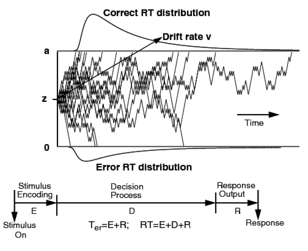
The diffusion model (Ratcliff, 1978; Ratcliff & McKoon, 2008; Ratcliff & Rouder, 1998, 2000; Ratcliff & Smith, 2004; Ratcliff, et al., 1999; Smith, 2000) provides an account of the cognitive processes involved in making simple, speeded, two-choice decisions. The model provides a unified account of all the features of the experimental data obtained in two-choice tasks, namely, accuracy (choice probabilities), the distributions of RT for correct responses and errors, and the relative speeds of correct responses and errors. The model (see Figure 1) distinguishes between the quality of the evidence entering the decision process and the overall amount of evidence needed to make a decision. It also distinguishes between the decision process and the other, nondecision processes that comprise RT.

Figure 1.

An illustration of the diffusion model. The 20 irregularly shaped paths illustrate variability in the process necessary to produce errors and the shapes of RT distributions. The process starts at a point z with drift rate v and terminates when it hits boundaries at 0 or a. The duration of the decision process, D, is added to the duration of stimulus encoding, E, and response output processes, R to give the total decision time. E+R=T_er the nondecision time.

In the model, decisions are made by a noisy process that accumulates information over time from a starting point, located at z, toward one of two response criteria, or decision boundaries, located at a and 0. When a boundary is reached, a response is initiated. The boundaries determine the overall amount of evidence needed for each of the two responses. The rate of evidence accumulation, or drift rate, is denoted v. The drift rate is determined by the quality of the sensory information extracted from the stimulus in perceptual tasks and by the goodness-of-match between the test item and memory in recognition memory and lexical decision tasks. The mean of the distribution of the nondecision component, which comprises encoding, response selection, and response execution processes, is denoted T_er. The unpredictable fluctuations in the sample paths of the diffusion process depicted in Figure 1 reflect moment-to-moment effects of noise in information accumulation on individual trials (these are from a random walk simulation of the diffusion process, see Ratcliff, 1978, for a description of the relationship between random walk and diffusion processes). The cumulative effect of such noise means that processes with the same drift rate will terminate at different times and sometimes at the wrong boundary. Variability in the times at which the processes finish leads to RT distributions; variability in the boundary at which they finish leads to errors.

The values of the components of processing (i.e., drift rates, decision criteria, starting points, and nondecisional times) vary from trial to trial. This variability is an expression of the idea that the parameters or operating characteristics of the decision process vary dynamically across trials (Laming, 1968; Ratcliff, 1978; Vickers, 1978). Drift rates are assumed to be normally distributed across trials with standard deviation η; starting points are uniformly distributed with range s_z, and nondecisional times are also uniformly distributed with range s_t. In addition, there are so-called "contaminant" responses. These are slow outliers that arise on a small proportion of trials due to inattention or lack of preparation and are assumed not to reflect the processes of interest. To accommodate these responses, we assume that, on some proportion of trials, (p_o), a random delay is added to the decision time. In fitting data, the random delay is assumed to be uniformly distributed between the minimum and the maximum RTs for each experimental condition. The assumption of uniformity is not critical, however, because recovery of diffusion model parameters is robust to variations in the form of distribution assumed for the delay (Ratcliff, 2008).

The values of all the parameters, including the variability parameters, are estimated from data by fitting the model to all conditions of an experiment simultaneously (as described shortly). The model can be seen as decomposing accuracy and RT for correct and error responses into its underlying components of processing. The model has been successful in accounting for data from all of the two-choice RT tasks described above, as well as for a wide variety of other experimental manipulations (Gomez, Ratcliff, & Perea, 2007; Ratcliff, 1988, 2008; Ratcliff & Rouder, 1998, 2000; Ratcliff & Smith, 2004; Ratcliff, Thapar, Gomez, & McKoon, 2004; Ratcliff, Thapar, & McKoon, 2001, 2003, 2004, 2006; Smith & Ratcliff, 2009; Smith, Ratcliff, & Wolfgang, 2004; Thapar et al., 2003; Voss, Rothermund, & Voss, 2004; Wagenmakers, Ratcliff, Gomez, & McKoon, 2008).

Like other sequential-sampling models (Ratcliff & Smith, 2004), the diffusion model assumes that the decision process begins to accumulate evidence at some random time after stimulus onset. For the diffusion model, this occurs just before the first time at which the predicted RT distributions begin to differ from zero. To date, however, the mechanism that initiates evidence accumulation has not been identified; that is, we do not fully understand how the process of evidence accumulation is turned on. Smith and Ratcliff (2009) described two possible candidates for such a mechanism. The first assumes that the noise in the accumulation process arises as the result of stimulus encoding. There is no accumulation prior to encoding because in the absence of a stimulus the mean and variance of the matching process are both zero. The onset of evidence accumulation is controlled by a change in the variance of the within-trial noise from a zero to a nonzero value. This is described mathematically in the model by a change in a quantity called the diffusion coefficient, which determines the fluctuations in the accumulation process shown in Figure 1. Although a change in variance will usually be accompanied by a change in mean, it is the change in variance that is critical, because the processes in Figure 1 will begin to diverge from their starting points as soon as the variance changes from zero. A zero mean and a nonzero variance will occur in the case of a wholly uninformative (zero discriminability) stimulus. If presented with such a stimulus, the decision process will accumulate noise and will terminate at either boundary equally often, in finite time. The random fluctuations in the accumulation process, which arise as the result of noise, are an essential part of the model, as they allow it to predict errors and the shapes of RT distributions.

A second, more biologically motivated, possibility is a generalized release from inhibition. This alternative assumes that there is noise in the system prior to stimulus presentation but it is not accumulated, because accumulation is opposed by inhibitory processes. When the inhibition is released, accumulation begins. Unlike the first alternative, in which the noise entering the decision process changes with stimulus onset, the effect of release from inhibition is to change the way in which noisy information is accumulated. Whereas the noise in the first alternative arises from stimulus encoding, in the second alternative it is inherent in the decision process itself, but its effect on the mean and variance of the process increases when inhibition is released. Although these are theoretically different mechanisms, their behavioral effects are likely to be very similar or indistinguishable. We discuss these mechanisms in more detail subsequently.

Model Fitting and Displaying Fits: Quantile Probability Functions

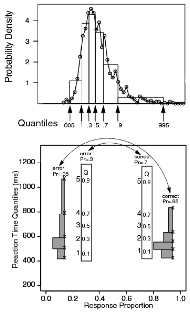
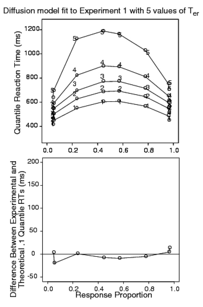
In the standard diffusion model, the predictions are based on the assumption that the only parameter of the model that changes across stimulus conditions is the drift rate. Fits of the model to data can be depicted most compactly as quantile probability plots (Ratcliff, 2001). In these plots, the .1, .3, .5, .7, and .9 quantiles of the RT distribution are plotted on the y-axis as a function of the response proportion on the x-axis. The quantile probability plot turns the distribution "on its end," in the sense that the shape of the distribution is represented on the y-axis rather than the x-axis, as in the usual RT histogram. In the physical and biological sciences plots of this kind are called parametric plots. Such plots provide a graphic way of showing how the behavior of a two- dimensional system changes as a function of a single system control parameter. Here the two dimensions of the system are the dependent variables, RT and accuracy (i.e., choice probability), and the control parameter is stimulus discriminability. The value of this way of representing the data is that it shows how distribution shape and accuracy jointly vary as a function of the stimulus condition.

Figure 2 illustrates this way of plotting the data. The top panel shows two ways of representing the information in a single distribution: as a frequency polygon (the circles connected with the jagged line), and as an equal-area histogram. Both of these representations are approximations to the RT probability density function. In the histogram, there is a probability mass of .2 between the .1, .3, .5, .7, and .9 quantiles, and .1 outside of each of two extreme values. The distribution of mass can be represented as a set of rectangles, each with an area of .2 and a base equal to the difference in the adjacent quantiles. The two extremes are represented as rectangles of area .1. The bases of the rectangles representing the extremes of the distribution (its leading edge and its tail) are equal to the difference between the .005 and .1 quantiles and the difference between the .9 and .995 quantiles, respectively. The .005 and .995 quantiles are used to mark the extremes of the distribution because they provide relatively stable estimators of the fastest and slowest RTs. Because each of the rectangles has an area of .2 (with the remaining .2 shared between the two extremes), all of the information about distribution shape is carried by the spacing between the quantiles. As can be seen, the equal-area histogram captures the overall shape of the distribution (i.e., its location, spread, and skewness) as well as does the frequency polygon.

Figure 2.

The top panel shows a RT distribution as a frequency polygon, along with a quantile RT distribution with equal area rectangles drawn between the .1, .3, .5, .7, and .9 quantile RTs and rectangles with half the area outside the .1 and .9 quantile RTs. The bottom panel shows a quantile probability plot with the proportion of responses for that condition on the x-axis and quantile RTs plotted as x’s on the y-axis (x’s on the outermost pair, and digits on the innermost pair, with 1=.1 quantile RT, 2=.3 quantile RT, 3=.5 quantile RT, 4=.5 quantile RT, and 5=.9 quantile RT). Equal areas rectangles are drawn between two of the sets of the quantiles to illustrate how to interpret RT distribution shape in the plot (these are comparable to the distribution in the top panel). Two conditions are shown, one with accuracy at .95 with the error proportion .05 and the other with accuracy .7 with the error proportion .3. The correct/ error relationship is illustrated by double ended arrows pointing to the pairs. In the plots of data, digit alone are used to present values of the quantile RTs.

The bottom panel of Figure 2 shows how the information in a family of distributions can be represented in a single plot. The plot illustrates the relationship between the histograms (the gray rectangles) and the quantiles that summarize them (the x-symbols). It also shows how the important features of the distribution shape are carried by the spacing of the quantiles. The quantiles for each pair of distributions of correct responses and errors are plotted against the associated choice probabilities. If the probability of a correct response for a particular stimulus discriminability is p, the quantiles of the distribution of correct responses are plotted in a vertical column against p on the x-axis and the quantiles of the distribution of errors are plotted against 1 - p. In the figure, this correspondence is illustrated by the double-ended arrows connecting pairs of conditions. This means that correct responses appear (usually) on the right of .5 point on the x-axis and errors appear on the left. In plots of this kind, the outermost pair of distributions in the figure are the errors and correct RTs for the easiest stimulus condition and the innermost pair are the errors and correct RTs for the most difficult stimulus condition.

In quantile probability plots of data, the quantiles on the left of the plot are typically much more variable than are those on the right. This is because the quantiles on the left are for error responses and are based on fewer observations than are the quantiles for correct responses on the right. Furthermore, when quantiles are averaged across subjects, the estimated quantiles of the error distributions will be disproportionately influenced by subjects with high error rates for highly discriminable stimuli. This is because some subjects may not have made errors in these extreme conditions and so will not contribute to the estimated quantiles. Error RTs to highly discriminable stimuli and the tail quantiles of error distributions should therefore be accorded relatively little weight in evaluating model fits. In fitting the models to data, error quantiles in which there are no data for some subjects are excluded from the fit.

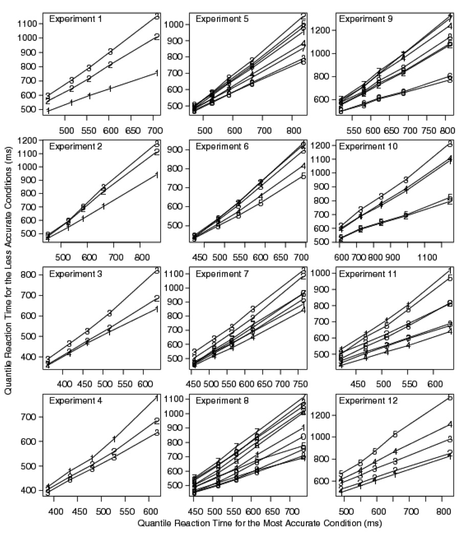
Ratcliff and McKoon (2008) showed that quantile-quantile plots of distribution pairs are approximately linear, implying that distribution shape is largely invariant across experimental conditions, both in data and in model predictions. In the general discussion we present such plots for all the experiments that support this contention.

The diffusion model is fit to data by minimizing the Pearson chi-square statistic using the Nelder-Mead SIMPLEX algorithm (Nelder & Mead, 1965). This algorithm adjusts the parameters of the model iteratively until it finds the parameter values that give the minimum chi-square (see Ratcliff, 2008; Ratcliff & Tuerlinckx, 2002, for further details of the fitting procedure). The data used to fit the model are the .1, .3, .5, .7, and .9 quantile RTs for correct responses and errors for each experimental condition, together with their associated response probabilities. For each candidate set of parameter values, the diffusion model predicts the proportion of probability mass falling into the bins formed from adjacent quantiles. These expected proportions are compared to the actual proportions falling between the 0, .1, .3, .5, .7, .9, and 1.0 quantiles (i.e, .1, .2, .2, .2, .2, and .1, respectively). Summing the values of (Observed-Expected)²/Expected over all conditions and multiplying by the number of observations gives a single chi-square value, which is minimized as a function of the model parameters.

In this article, we fit the diffusion model to quantile-averaged group data. In fitting the data from many experiments we have found that the parameter values obtained from fits to group data agree fairly well (within two standard errors) with the averages of parameters obtained from fitting the model to individual subject data (Ratcliff, Thapar, Gomez, & McKoon, 2004; Ratcliff, Thapar, & McKoon, 2001, 2003, 2004, 2006; Thapar et al., 2003). We now present the results of nine new experiments and reanalyze the results from three published experiments. These experiments explore the conditions under which the leading edge of the RT distribution shows a substantial change with changes in discriminability.

Experiments

In all of the experiments, the proportion of contrast-reversed pixels was manipulated to produce a range of accuracy values from near ceiling (100% correct) to near floor (50% correct). In practice, the values ranged from around 95% correct to around 60% correct in most cases. This large range of RT and accuracy values was designed to provide the most stringent test possible of the diffusion model.

General Methods

One of two tasks was used in most of the experiments. In the first task, subjects were presented with one of two letters and had to make a choice between the two. The stimulus letters were all capitals 0.85 degrees high and 0.6–1.1 degrees wide. The stimulus letter was presented in white on a black 64 × 64 pixel background (subtending 3.0 × 3.0 degrees). Stimuli were degraded either by randomly reversing the contrast polarity in some proportion of the pixels in the pixel array or by masking the stimulus after a brief exposure. In the static version of the task, the stimulus consisted of a single frame that was presented until a response was made. In the dynamic version of the task, the stimulus consisted of a sequence of frames presented at a frame rate of 60 Hz or 100 Hz, with a new set of contrast-reversed pixels randomly chosen on each frame. The letter was presented in the center of the random array. Subjects responded with the / key for the right hand letter choice and Z key for the left hand letter choice. The same two letters were used for a block of trials; these were then replaced with another letter pair for the next block. Each pair of letters was used again in a later block, but with the mapping of letters to the left and right hands reversed. To indicate the mapping between letters and response keys, two letters corresponding to the two choices were displayed on the left and right sides of the screen (left letter for the "Z" key and right letter for the "/" key) and were continually on the screen throughout the block of trials.

In the second task, subjects were presented with a homogeneous, random 60×60 array of black and white pixels (subtending 3.2 by 3.2 degrees), in which the proportion of black to white pixels was systematically varied. Subjects judged whether the array was light, with more white pixels than black, or dark, with more black pixels than white, and responded using the / and Z keys, accordingly. In the static version of the task, the stimulus consisted of a single frame that remained present until the response. In the dynamic version, the stimulus consisted of a sequence of frames presented at a frame rate of 60 Hz or 100 Hz, with a new set of contrast-reversed pixels randomly chosen on each frame.

The experiments were run by a real-time Linux system on Pentium 4 class computers. Stimuli were presented on Dell Ultrascan P780 CRT monitors with 17 inch viewing areas. Subjects viewed the stimuli at a distance of 57 cm; at this distance, 1 cm on the screen subtended one degree of visual angle. The stimuli were presented on a 320 × 200 pixel background, which subtended 15.5 × 8.8 degrees at the specified viewing distance. The pixel size was 0.05 × 0.05 degrees, except in Experiment 11, where it was 0.025 × 0.025 degrees.

In most of the experiments, a block consisted of 96 trials. The target stimulus presented on each trial was chosen randomly, with the restrictions that the two response alternatives and the different levels of stimulus discriminability (proportions of contrast-reversed pixels) were presented equally often in each block. A block lasted a little more than 2 minutes and subjects were encouraged to take brief rest breaks between blocks. There were 14 block of trials. In the data analysis, the first block of trials and the first response in each block were discarded.

Subjects

Undergraduate students from Ohio State University participated in the experiments for credit in an introductory psychology class. All of the experiments tested subjects for one 45 minute session. Between 14 and 20 subjects were used in each experiment.

Procedure

Subjects were instructed to respond as quickly and accurately as possible. Incorrect responses were followed by an "ERROR" message displayed for 300 ms. No feedback was provided for correct responses. In addition, responses longer than 1800 ms were followed by a "TOO SLOW" message displayed for 300 ms, and responses faster than 250 ms were followed by a "TOO FAST" message displayed for 1000 ms (to discourage fast guessing). The response to stimulus interval was 500 ms.

Experiment 1: Letter discrimination in dynamic random pixel noise

White letters were presented on a black background with the proportion of contrast- reversed pixels (in both the letter and background) systematically varied. The set of contrast- reversed pixels was randomized in each consecutive 10 ms frame to create a dynamic stimulus.

Method

Twenty subjects participated in this experiment. The stimuli were white letters displayed in the center of the computer screen against a dark background. Letters were paired so as to be visually dissimilar to each other. The pairs were F/Q, P/U, W/K, B/N, T/X, G/V, and L/R.

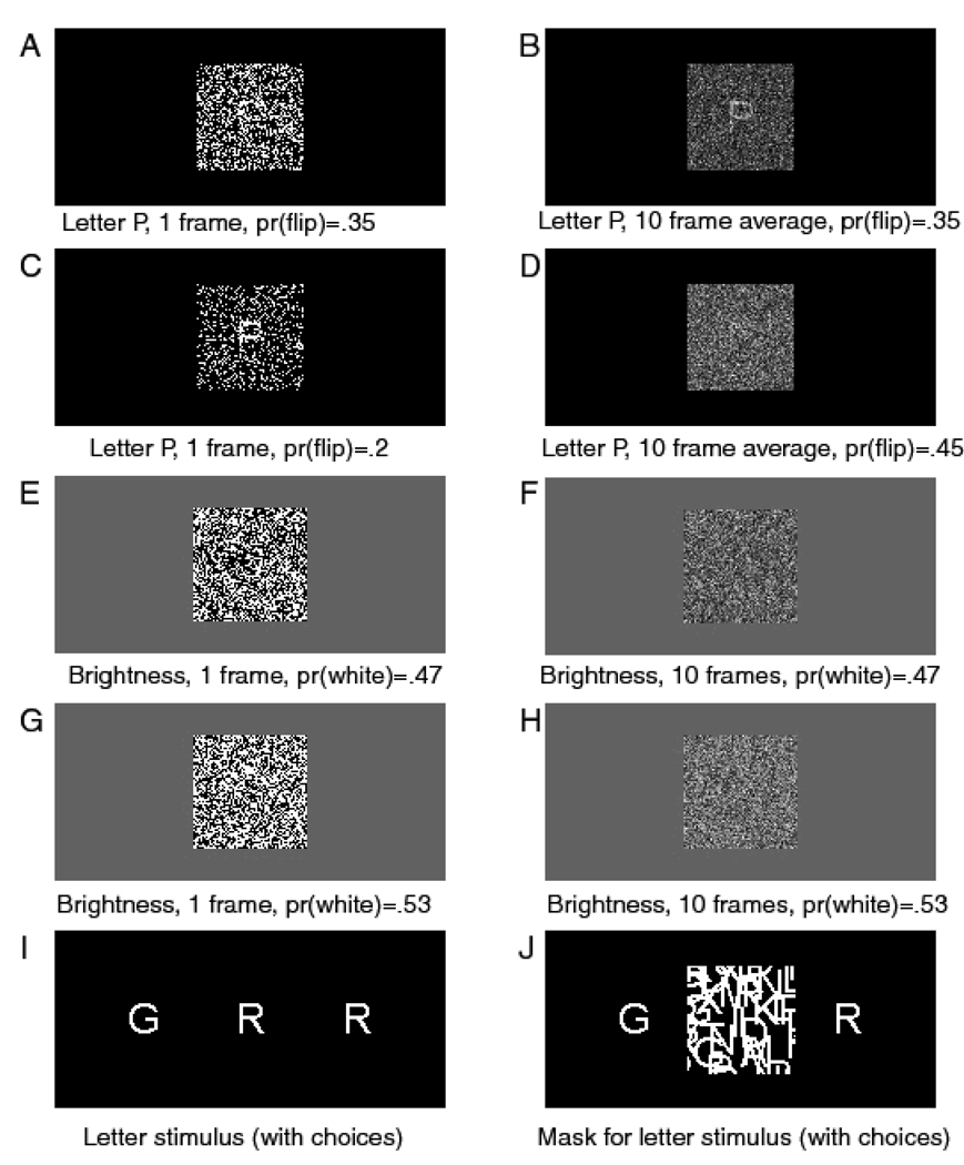
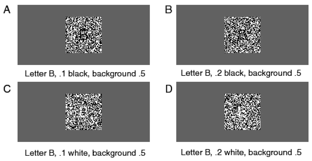
Each trial began with a fixation point in the center of the screen, displayed for 500 ms, then the target letter was displayed in dynamic noise. The onset of the noise and the onset of the stimulus coincided. Subjects were instructed to press the ‘/’ key on the keyboard if the right hand letter had been presented and the ‘Z’ key if the left hand letter had been presented. There were four levels of stimulus discriminability produced by inverting .35, .4, .45, and .475 of the pixels in the display. On each frame of the display, a different random set of pixels was inverted. The frame rate was 10 ms per frame. Figures 3A and 3C show two examples of the stimuli for a single frame; Figures 3B and 3D show the averages over 10 frames. Because successive stimulus frames would have been integrated by the visual system, the 100 ms averages are likely to be more representative of what the subjects actually perceived. The trial structure, stimulus randomization, and experimental procedure were as described in the General Methods section above.

Figure 3.

Examples of the stimuli from Experiments 1–4.

Results

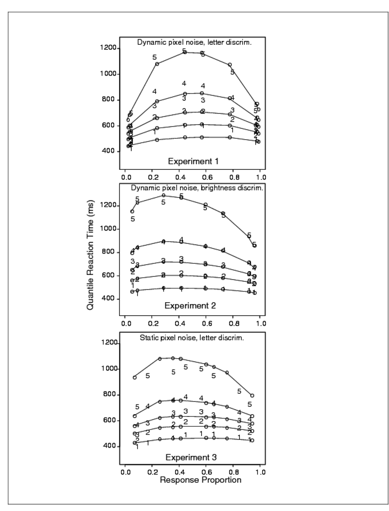
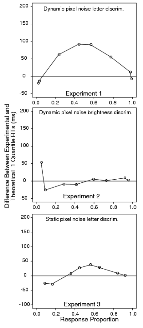
Trials with RTs larger than 2500 ms or less than 270 ms were discarded (less than .9% of the data, .3% were fast responses). Correct responses to left hand letter stimuli were pooled with correct responses to right hand stimuli for each level of stimulus discriminability. Error responses were combined in a similar way. From the pooled RTs, quantile RTs were produced. The top panel of Figure 4 shows the quantile probability plot for Experiment 1. The empirical RT quantiles are denoted by the digits 1 through 5 and the predictions from the diffusion model are denoted by o’s joined by lines (in the model, only drift rate is allowed to vary across experimental conditions). From the plot, it can be seen that accuracy for the 0.35, 0.4, 0.45, and 0.475 proportions of inverted pixels was 0.96, 0.96, 0.79, and 0.57, respectively. The corresponding mean RTs for correct responses were 575, 615, 761, and 843 ms. The figure shows that the model misses the experimental 0.1 quantile RTs by up to 100 ms in the most difficult condition. Note that in this experiment (top panel) the accuracy levels for the two easiest conditions were almost the same, so the quantiles for these conditions appear almost superimposed on each other at the outer edges of the plot.

Figure 4.

Quantile probability plots for Experiment 1 (letter discrimination with dynamic random pixel noise), Experiment 2 (brightness discrimination with dynamic random pixel noise), and Experiment 3 (letter discrimination with static random pixel noise). The digits 1–5 represent the quantile RTs (as in Figure 2) from the data, and the circles are the predicted values of the quantile RTs from fits of the diffusion model.

The top panel of Figure 5 shows the difference between the observed .1 quantile and the diffusion model predictions. It shows that the discrepancy between the data and model increases with increasing task difficulty, reaching a maximum of around 100 ms in the .475 inversion condition. To estimate the standard error in the .1 quantile RT differences, we calculated the difference between the .1 quantiles for the 0.35 and 0.475 pixel proportions and then computed the standard error in the difference. The estimated standard error of the difference is 16 ms, so the misfit is a substantial one.

Figure 5.

Difference between experimental and diffusion model fit for the .1 quantile RTs for Experiment 1 (letter discrimination with dynamic random pixel noise), Experiment 2 (brightness discrimination with dynamic random pixel noise), and Experiment 3 (letter discrimination with static random pixel noise).

Experiment 2: Brightness discrimination with dynamic random pixel stimuli

Experiment 2 addressed the question of whether the large difference in the leading edge (.1 quantile) of the RT distribution across conditions in Experiment 1 would always be found with dynamic presentation, or only when the task requires discrimination of form. The experiment used a brightness discrimination in which stimulus presentation was dynamic, but no discrimination of form was required. Subjects made ‘dark’ or ‘light’ judgments to arrays of black and white pixels in which the proportion of black to white pixels was manipulated and in which different random samples of pixels were presented in consecutive frames.

Method

The stimulus was a 64×64 square of black and white pixels on a 320×200 pixel gray background. The pixel array subtended a visual angle of 3.5 degrees at a normal viewing distance of 57 cm. Eight different proportions of white pixels were used to give eight levels of brightness (four levels of discriminability). The proportions of white pixels were .38, .42, .47, .485, .515, .53, .58, and .62. A different random sample of pixels was presented in each consecutive, 16 ms frame. Examples of single frames are shown in Figures 3E and 3G; 10-frame averages are shown in Figures 3F and 3H.

There were 10 blocks of 96 trials in each experimental session, with each brightness level presented 12 times per block. Data from the first block of trials and the first response in each block were discarded from the analysis. Data were collected from 15 subjects.

Results

Trials with RTs longer than 2500 ms or shorter than 270 ms were eliminated (less than 3.5% of the data, 2.5% of these rejected trials came from fast guesses from two of the subjects - accuracy of their responses shorter than 270 ms was at chance, and .6% of the errors were slow responses). Light responses to light stimuli were combined with dark responses to dark stimuli at each of the four levels of discriminability (i.e., light responses to stimuli with .62 white pixels were combined with dark responses to stimuli with .38 white pixels, and so on). The middle panel of Figure 4 shows a quantile probability plot of the results. Accuracy values for the .38, .42, .47, and .485 stimulus conditions were .95, .92, .73, and .59 respectively; the corresponding mean RTs for correct responses were 623, 662, 741, and 764 ms. The plot shows that the fit of the diffusion model is extremely good.

The middle panel of Figure 5 shows the difference between the predicted and observed .1 quantiles of the RT distributions. Unlike Experiment 1, there is an almost perfect match between theory and data. The standard error of the difference between the .1 quantile RT for correct responses in the easiest and the most difficult conditions is 10 ms. The misses for the error distributions, shown on the left hand side of the figure, are larger and more variable, for reasons discussed previously. The number of observations in each of the error distributions is comparatively small and, because of individual differences in error rates, highly variable. This variability increases progressively from right to left across the function. For example, at the extreme left, the standard error in the .1 quantile is 43 ms, with two subjects producing no error responses at all.

Discussion: Experiments 1 and 2

The difference in the patterns of results for Experiments 1 and 2 is striking. The quantile probability plot for Experiment 1 shows a large bow in the .1 quantile function, whereas Experiment 2 does not. The bow reflects large changes in the leading edge of the RT distribution with changes in stimulus discriminability. We refer to this bowing of the .1 quantile subsequently as the "leading edge effect." If we fit the diffusion model under the assumption that the drift rate is constant over time and the decision process is turned on, on average, at the same time in each condition, the model’s predictions about the location of the leading edge are clearly falsified for Experiment 1, but confirmed for Experiment 2. Both experiments used dynamic stimuli, so it is not the dynamic nature of the stimuli per se that causes the misfit to the leading edge in Experiment 1.

The finding that dynamic noise produced a leading edge effect in letter discrimination but not brightness discrimination is consistent with our original hypothesis, which was that the effect arises from a combination of dynamic noise and the use of categorical stimuli (letters). However, an alternative hypothesis is that it is simply the categorical nature of the stimuli that causes the delay, and not the dynamic nature of the display. This did not seem plausible because Thapar et al. (2003) showed that presenting a letter and then masking it does not produce a change in the leading edge. (Their data are reanalyzed here as Experiment 4.) Another possibility is that it is not simply the fact that the stimulus is degraded, but the manner in which it is degraded, with random pixel noise, that is responsible for the leading edge effect.

To test this, in Experiment 3 we used a static display consisting of a letter in a single sample of random pixel noise. Our aim in carrying out this experiment was to ascertain whether the leading edge effect found with noise and categorical stimuli was dependent on the dynamic nature of the noise. We reasoned that if this experiment showed the same leading edge effect as Experiment 1, then it could be attributed to a combination of categorical stimuli and noise of any kind. If, however, there was no leading edge effect -- that is, if the diffusion model fits the data well -- then the effect must depend on the dynamic properties of the noise.

Experiment 3: Letter discrimination with static random pixel stimuli

Experiment 3 used a static version of the task used in Experiment 1. Subjects discriminated between pairs of letter stimuli that were degraded by having a proportion of the pixels in the letter and background contrast-reversed. Unlike the stimuli in Experiment 1, the stimuli in Experiment 2 each consisted of a single, noisy image that remained present until the response was made.

Method

The proportions of contrast-reversed pixels in the stimuli were .2 .275, .35, or .4. Examples of the stimuli are shown in Figure 3A and 3C. The proportions of reversed pixels were smaller than in Experiment 1 because the task was more difficult than it was with dynamic stimuli. In all other details, the experiment was the same as Experiment 1. Data were collected from 19 subjects.

Results

Data from trials with RTs longer than 2500 ms or shorter than 270 ms were discarded (less than 2.7% of the data, 2.3% fast responses). Left and right responses were pooled to obtain one distribution of correct responses and one distribution of errors for each level of stimulus discriminability. The bottom panel of Figure 4 shows the fit of the diffusion model as a quantile probability plot. From the plot, it can be seen that the accuracy for the .2, .275, .35, and .4 reversal conditions was .92, .84, .65, and .56 respectively. The corresponding mean RTs for correct responses were 575, 627, 687, and 720 ms. The o’s are the predictions from the diffusion model. The figure shows that there is again a leading edge effect, with the model missing the empirical .1 quantile by up to 40 ms in the most difficult stimulus condition.

The bottom panel of Figure 5 shows the difference between the data and the model prediction for 0.1 quantile. It shows a 40 ms miss in the condition in which .4 of the pixels were reversed. The standard error of the difference in the .1 quantiles for the easiest and most difficult conditions is 10 ms. Although the leading edge effect is not as large as in the dynamic noise case, it is systematic and significant. This means that it is not the difference between static and dynamic noise that is critical to producing the leading edge effect with letter stimuli; rather, it appears to be the combination of random pixel noise and categorical letter stimuli that is responsible for the discrepancy.

Experiments 4, 5, and 6: Letter Discrimination, Brightness Discrimination, and Motion Discrimination

We now reanalyze data from three published experiments; these experiments are labeled 4, 5, and 6 to aid reference. The model fits are presented in the same way as above. Two of the experiments used masks with static displays and the other used a dynamic motion discrimination task. These experiments show a series of other experimental manipulations that do not produce the mismatch between diffusion model predictions and data.

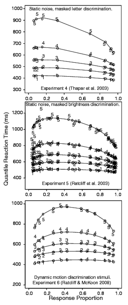
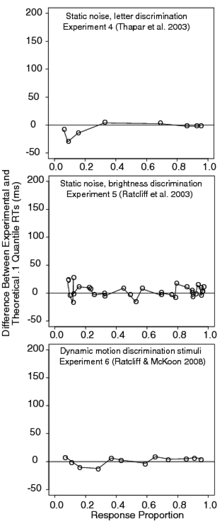
Experiment 4 was a letter discrimination task with masked stimuli (Thapar, Ratcliff, & McKoon, 2003). The stimuli were white letters on a black background, similar to those used in Experiment 2, except they were masked with randomly-oriented line segments after 10, 20, 30, or 40 ms. Examples of the stimulus and mask are shown in Figure 3I and 3J (except the mask had random lines instead of randomly placed letters). We analyze data from an accuracy instruction condition using a sample of college students (undergraduates at Northwestern University). The quantile probability plot is shown in the top panel in Figure 6. It shows that the diffusion model predicts these data quite well. The top panel in Figure 7 shows the difference between the predicted and observed .1 quantile. There is no systematic leading edge effect, except at the very left of the plot, where the error rates are very low and the errors of estimate are large.

Figure 6.

Quantile probability plots for Experiment 4 (letter discrimination with masking, from Experiment 1, young subjects, accuracy condition from Thapar et al., 2003), Experiment 5 (brightness discrimination with masking, from Experiment 1, young subjects, accuracy condition from Ratcliff et al., 2003), and Experiment 6 (motion discrimination from Experiment 1, Ratcliff & McKoon, 2008).

Figure 7.

Difference between experimental and diffusion model fit for the .1 quantile RTs for Experiment 4 (letter discrimination with masking, from Experiment 1, young subjects, accuracy condition from Thapar et al., 2003), Experiment 5 (brightness discrimination with masking, from Experiment 1, young subjects, accuracy condition from Ratcliff et al., 2003), and Experiment 6 (motion discrimination from Experiment 1, Ratcliff & McKoon, 2008).

Experiment 5 was a brightness discrimination task in which a static array of pixels was masked after 50, 100, or 150 ms (Ratcliff, Thapar, & McKoon, 2003). The stimulus was a static version of the one used in Experiment 2. The proportions of white pixels were .65, .575, .525, .475, .425, .35, giving three levels of stimulus discriminability (by combining bright responses to the .65 pixel condition with dark responses to the .35 white pixel condition and so on). The manipulation of the proportion of white pixels had a larger effect on performance than did the manipulation of stimulus duration. The fit of the diffusion model is shown in the middle panel of Figure 6 and the difference in the predicted and observed .1 quantile is shown in the middle panel of Figure 7. As for Experiment 4, these plots show good agreement between the predictions of the diffusion model and the data, with no evidence of a systematic leading edge effect.

Experiment 6 was a motion discrimination task, originally reported as Experiment 1 of Ratcliff and McKoon (2008). In this task, some proportion of dots in an array of randomly-moving dots moved coherently in a left or right direction. The remaining dots moved incoherently; that is, their motion in successive frames was uncorrelated. The difficulty of the task was manipulated by varying the proportion of dots that moved coherently. In Ratcliff and McKoon’s experiment, the dots were 1 pixel (0.054 degrees) square and moved at a rate of 13 deg/second. The proportion of the dots that moved coherently varied from .05, .1, .15, .25, .35, to .50.

The quantile probability functions for the data and diffusion model fit are shown in the bottom panel of Figure 6. The bottom panel of Figure 7 shows the difference between the predicted and observed .1 quantile. Figure 6 shows that the fit of the diffusion model is excellent and Figure 7 shows there is no systematic leading edge effect. These experiments show that there are no mismatches between the diffusion model predictions and the RT distribution data for these three perceptual tasks. Letter discrimination with backward masking apparently does not operate in the same manner as letter discrimination with random pixel noise and does not produce a leading edge effect. Brightness discrimination with masked, static stimuli shows the same pattern of results as brightness discrimination with dynamic displays. Neither task produces a leading edge effect. Further, motion discrimination with dynamic stimuli again shows good agreement between the diffusion model predictions and data, and again shows no leading edge effect.

Experiment 7: Blocks of static letter and brightness discrimination

The experiments we have described above with static and dynamic noise used different stimuli. Therefore it is possible that the different patterns of results found for the different tasks were due to differences in the stimuli rather than differences in the kinds of judgment made about them. In Experiment 7, the same stimuli were used for brightness discrimination and letter discrimination, with switches between tasks made in consecutive blocks of trials. The stimuli were white or black letters presented on a random background comprising 50% black and 50% white pixels. As in Experiments 1 and 2, task difficulty was varied by varying the proportion of contrast- reversed pixels in the letter only (Experiments 1 and 2 reversed contrast in both the letter and background). The task was static; only a single stimulus image was presented on any trial. This remained present until the response was made.

Method

The proportion of inverted pixels was .01, .1, .15, and .2 for the letter discrimination task and .1, .2, .3, and .4 for the brightness discrimination task. These proportions are lower than the corresponding proportions for Experiments 1 and 3. This is a reflection of the different ways in which the stimuli were constructed in the two tasks. Because stimuli in Experiment 7 were presented against a background composed of 50% black and 50% white pixels, effective stimulus contrasts were lower in this task than in Experiments 1 and 3, in which the proportion of inverted pixels in the background was same as in the stimulus letter. Examples of the stimuli are shown in Figure 8. In the brightness discrimination task, only the brightness of the letter was judged, while in Experiment 2 the brightness of the whole pixel array was judged.

Figure 8.

Examples of stimuli for Experiment 7.

In consecutive blocks of trials, subjects decided which of the two target letters was presented or whether the letter was light or dark. For the light/dark discrimination, instead of presenting the two response alternatives to the right and left of the array, a white or a black rectangle replaced the letters. The pairs of letters presented were F/Q, P/L, W/K, B/N, T/X, and G/ R. Data were collected from 18 subjects.

Results

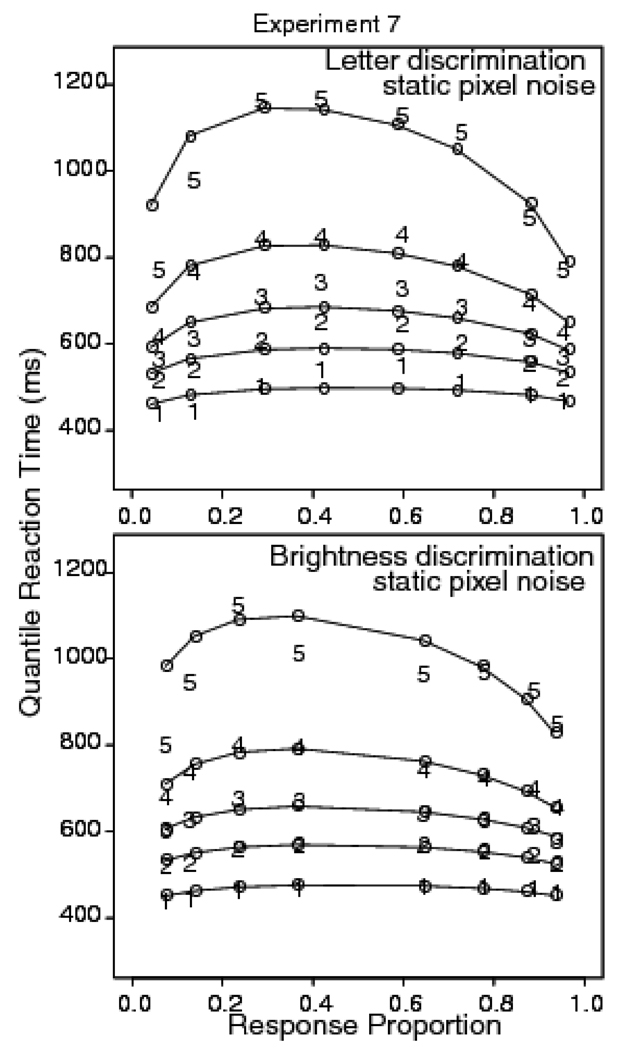
Trials with RTs larger than 2500 ms or less than 270 ms were discarded (less than 1.0% of the data, .3% fast responses). For letter discrimination, the accuracy values in the .01 .1, .15, and .2 reversal conditions were .95, .87, .72, and .59, respectively. The corresponding mean RTs for correct responses were 592, 651, 746, and 798 ms. For brightness discrimination, the data were pooled across bright and dark responses at each discriminability level. Accuracy values for the .1, .2, .3, and .4 reversal conditions were .93, .88, .77, and .64; the corresponding mean RTs for correct responses were 614, 649, 676, and 691 ms.

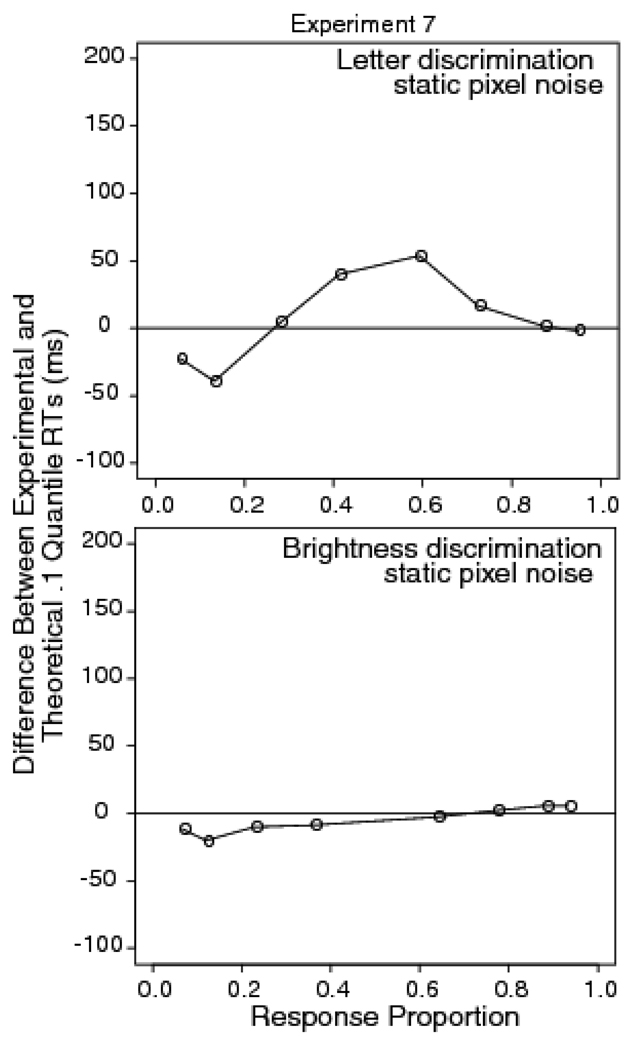
Figure 9 shows quantile probability plots for the letter and brightness discrimination tasks. For the letter discrimination task, the diffusion model predictions miss the leading edge of the distribution, while for the brightness discrimination task, the model fits the leading edge well. Figure 10 shows the difference between data and the diffusion model predictions for the two tasks. For the brightness discrimination task, there is almost no miss for correct responses (points to the right of .5 on the x-axis) while for the letter discrimination task, the miss is about 60 ms. The standard error of the difference between the .1 quantiles for the .01 and .2 reversal conditions in the letter discrimination task was 10 ms. These results show that with the same stimuli, but differences in the kind of judgment required, there is a leading edge effect for the letter discrimination task, but none for the brightness discrimination task. This shows that it is the task that is responsible for the miss between diffusion model predictions and data and not some subtle property of the stimulus.

Figure 9.

Quantile probability plots for Experiment 7. The stimuli were letters in dynamic random pixel noise and different blocks of trials had subjects judge the brightness of the letter (it could be brighter or darker than the background) or which of the two letter choices was presented.

Figure 10.

Difference between experimental and diffusion model fit for the .1 quantile RTs for Experiment 7. The stimuli were letters in dynamic random pixel noise and different blocks of trials had subjects judge the brightness of the letter (it could be brighter or darker than the background) or which of the two letter choices was presented.

Experiment 8: Mixed dynamic letter discrimination, static letter discrimination, and letter discrimination with masking

An alternative hypothesis is that subjects change some aspect of the decision process as a function of the demands of the stimulus. This could be viewed as a strategic shift, in which they delay initiation of the decision process when a series of stimuli are difficult to resolve perceptually. If this were correct, then mixing different kinds of trials -- namely, those with dynamic pixel noise, those with static pixel noise, and those with static masked displays -- should induce the same delay in the leading edge of the RT distribution for all stimulus types.

Method

Each of the tasks required subjects to decide which of two letters had been presented, as in Experiments 1, 3, and 4. Examples of the stimuli are shown in Figure 3. Three kinds of stimuli were randomly intermixed within each block, so that any of the three trial types could occur on any trial. All three trial types presented white letters on black backgrounds. In the static displays, .2 .275, .35, or .4 or the pixels were contrast-reversed, as in Experiment 3. In the dynamic displays, .35, .4, .45, or .475 of the pixels were contrast-reversed, as in Experiment 1. In the masked displays, the stimulus was masked with randomly oriented letters after 20, 40, 60, or 80 ms (the frame rate for this experiment was 10 ms). Data were collected from 18 subjects.

Results

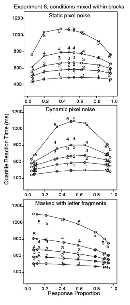
Trials with RTs longer than 2500 ms or shorter than 270 ms were discarded (less than 1.2% of the data, 1.1% were fast responses). For letter discrimination with static noise, the accuracy values in the .2 .275, .35, and .4 pixel reversal conditions were .94, .81, .64, and .53; the corresponding mean correct RTs were 584, 665, 741, and 783 ms. For letter discrimination with dynamic noise, the accuracy values in the .35, .4, .45, and .475 reversal conditions were .93, .91, .68, and .54; the corresponding mean correct RTs were 576, 632, 776, and 804 ms. For masked letter discrimination, the accuracy values in the 20, 40, 60, and 80 ms exposure duration conditions were .93, .87, .78, and .59; the mean correct RTs were 564, 574, 662, and 718 ms.

Figure 11 shows the quantile probability plots for the three tasks. The results show reasonably good fits for the masked letter discrimination task, with a few misses in the .9 quantile RTs (which are more variable than lower quantile RTs) and in the extreme error condition, which does not contain enough responses to estimate quantiles for some subjects. For the static and dynamic pixel noise letter discrimination tasks, there are appreciable misses between the diffusion model prediction for the .1 quantile RT and the experimental data.

Figure 11.

Quantile probability plots for Experiment 8. Three tasks were randomly mixed within blocks, letter discrimination with dynamic random pixel noise, letter discrimination with static random pixel noise, and letter discrimination with masking.

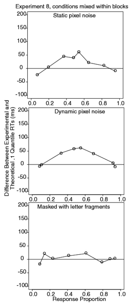
Figure 12 shows plots of the differences between the data and the model for the .1 quantile. For the masked letter discrimination task, the largest miss in the .1 predictions is 18 ms. The standard error of the difference between the .1 quantiles for the 40 ms and 10 ms exposure durations is 10 ms, so the difference is not significant. In contrast, the static pixel noise condition and the dynamic pixel noise conditions show misses in the .1 quantile predictions of 71 and 70 ms respectively. These misses are substantial because the standard error of the difference in the .1 quantile for the easiest and most difficult conditions is 21 and 23 ms for static and dynamic stimuli, respectively.

Figure 12.

Difference between experimental and diffusion model fit for the .1 quantile RTs for Experiment 8. Three tasks were randomly mixed within blocks, letter discrimination with dynamic random pixel noise, letter discrimination with static random pixel noise, and letter discrimination with masking.

These results show that mixing random pixel noise in letter discrimination with masked stimuli does not produce a uniform leading edge effect for all stimulus types. If random pixel noise induced a strategy of delaying responding to difficult stimuli, then we would expect that such a delay would be induced for masked letter discrimination. The results show that this did not occur.

Experiments 9 and 10: Pedestal experiments

Smith and Ratcliff (2009) proposed that the leading edge effect is a function of the contrast energy of the stimulus. Contrast energy is defined as the squared deviation of the stimulus from its background, summed over the area and duration of the stimulus. Smith and Ratcliff argued that contrast energy is a measure of perceptual salience, that is, of how much a stimulus stands out from the background. Salience differs from discriminability, which is a function of stimulus similarity, or the confusability of the stimulus alternatives. They proposed that decision time is determined by discriminability and that the leading edge is determined by salience. Smith and Ratcliff compared RT distributions from two similar attentional cuing paradigms, one from an experiment by Smith, Ratcliff, and Wolfgang (2004) and the other from an experiment by Gould, Wolfgang, and Smith (2007, Experiment 1). In both paradigms, subjects discriminated between low-contrast, sinusoidal grating patches, presented unpredictably at one of three locations on a uniform background. In one paradigm, stimuli were localized spatially and temporally by surrounding them with four short, high-contrast line segments arranged in the shape of a cross (termed "fiducial crosses" by Gould et al.) In the other paradigm, stimuli were localized by presenting them on top of circular, 15%- contrast, luminance pedestals. Theoretically these manipulations should have had the same effect, of localizing the decision to a particular region of the display. Consistent with this, the attentional effect of the two manipulations was the same: When stimuli were unmasked, there was no cuing effect in accuracy and a significant effect in RT with both pedestals and fiducial crosses. However, their effect on RT distributions was different. When stimuli were localized with fiducial crosses, there was a leading edge effect; when they were presented on top of pedestals, there was no effect.

Smith and Ratcliff (2009) presented a model in which the stimulus information in the grating patch is gated into VSTM by the contrast energy in the stimulus. In this model, the decision process is turned on by the formation of the VSTM trace, either by progressively increasing within- trial noise, or by releasing inhibition in the accumulation process. (They implemented the former alternative in the model, but not the latter.) The location of the .1 quantile predicted by the model depends on the rate of VSTM formation: Slowing VSTM formation delays the onset of the decision process and shifts the RT distribution to the right. This rate, in turn, depends on the energy in the stimulus compound. When pedestals are used the compound consists of the patch and pedestal; when no pedestal is used the compound consists of the patch alone. Because the energy in the compound is dominated by the energy in the pedestal, the model predicts little or no change in the rate of VSTM formation with changes in contrast in the pedestal task, but large changes in the fiducial task. It therefore predicts no leading edge effect in the former task but a large effect in the latter task. This is what the data showed.

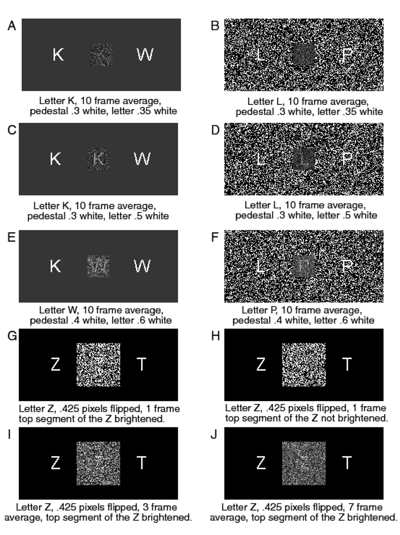
Experiments 9 and 10 used a version of the pedestal task, as shown in Figure 13, panels A through F. These experiments were designed to test the generality of Smith and Ratcliff’s (2009) hypothesis that a burst of uninformative contrast energy at stimulus onset initiates evidence accumulation by the decision process. Whereas the pedestal task of Smith and colleagues used static presentation and pedestals consisting of a localized increase in mean luminance, we used dynamic presentation and pedestals consisting of patches of random pixels whose contrast energies differed from that of the surrounding display. The goal of this manipulation was to test whether a burst of contrast energy at stimulus onset would eliminate the leading edge effect that was found with dynamic presentation.

Figure 13.

Examples of stimuli for Experiments 9, 10, and 11.

We compared pedestals whose mean luminances were either slightly greater than, or slightly less than, or the same as that of the surrounding display. The aim of this manipulation was to compare different ways of presenting the energy burst at stimulus onset. In the first condition it was carried by a luminance increment, in the second by a decrement, and in the third, by a transient in contrast energy that produced no change in local mean luminance. As all of these manipulations produced large changes in contrast energy at stimulus onset they should, according to the hypothesis of Smith and Ratcliff (2009), have had similar effects on the leading edge. We also compared the effects of placing the stimulus and pedestal on a uniform gray background (Experiment 9) and on a nonuniform, black and white pixel array (Experiment 10). When viewed statically, in Figure 13, the pedestal appears as a square filled with random pixels whose mean luminance is greater than, less than, or the same as the luminance of the background. When the background is composed of random pixels, the pedestal appears as a transparent gray square through which the background is visible. When viewed dynamically (see http://star.psy.ohio-state.edu/percept_stimuli.html for examples) the pedestal appears as a localized energy transient at stimulus onset. When the background was a random pixel array, pedestals of the same mean luminance as the surrounding display were visible only when viewed dynamically. In all conditions, the stimulus was a letter in dynamic noise, as in Experiment 1. Unlike Experiment 1, however, the onset of the letter was marked, both spatially and temporally, by the onset of the pedestal.

Method

The stimuli were white letters on a black background, presented on a 64×64 pixel, dynamic noise pedestal. A new sample of random pixels was presented in every 16.67 ms frame, as described in the General Methods section. The stimulus and pedestal were presented at the center of a 320×240 pixel, rectangular region. This region was a uniform 30% grey in Experiment 9 and a homogeneous array of .3 white pixels and .7 black pixels in Experiment 10. We compared three conditions in which the mean luminance of the pedestal was varied. In one, it contained .25 white pixels, which was a little darker than the background. In another, it contained .3 white pixels, which was the same as the background, and in the third it contained .4 white pixels, which was a little lighter than the background. The target was a white letter whose proportion of white pixels exceeded that of the background by .05, .1, or .2. Data were collected from 17 subjects in Experiment 9 and 14 subjects in Experiment 10.

Results

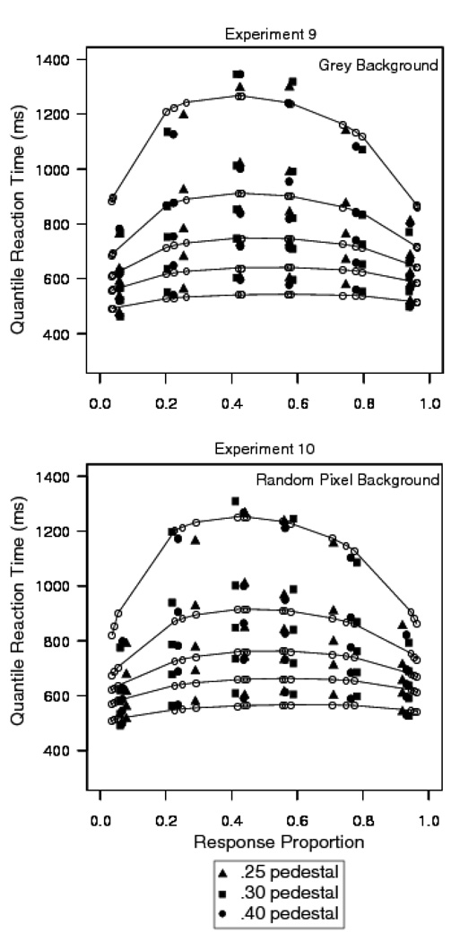
Trials with RTs longer than 2500 ms or shorter than 270 ms were discarded (less than .8% of the data for Experiment 9, .3% were fast responses, and less than 1% of the data for Experiment 10, .7% were fast responses). For Experiment 9, there was a small difference in both accuracy and mean RT as a function of mean pedestal luminance. For pedestal luminances (i.e., proportions of white pixels) of .25, .3, and .4, the accuracy values were .77, .76, and .75 and the mean RTs were 764, 765, and 791 ms respectively. The effect was not significant for accuracy, F(2,26)=2.8, p>.05, but was significant for mean RT, F(2,26)=13.2, p<.05. There was a large difference in accuracy and mean RT as a function of letter luminance for the .05, .1, and .2 luminance increment conditions. Accuracy values in these conditions were .58, .77, and .94 and mean RTs were 889, 793, and 637 ms respectively. The effect was significant for both accuracy, F(2,26)=525.9, p<.05, and mean RT, F(2,26)=91.1, p<.05.

For Experiment 10, there was a small difference in accuracy and mean RT as a function of mean pedestal luminance. For the .25, .3, and .4 pedestal luminances, accuracy values were .76, .75, and .73 and mean RTs were 782, 784, and 806 ms respectively. The effect was significant for both accuracy, F(2,26)=10.1, p<.05, and mean RT, F(2,26)=7.7, p<.05. There was a large difference in accuracy and mean RT as a function of stimulus contrast for the .05, .1, and .2 luminance increment conditions. Accuracy values were .57, .75, and .93 and mean RTs were 881, 823, and 668 ms respectively. The effect was significant for both accuracy, F(2,26)=494.9, p<.05, and mean RT, F(2,26)=70.1, p<.05. In neither experiment was the interaction between stimulus contrast and pedestal contrast significant for either accuracy or mean RT.

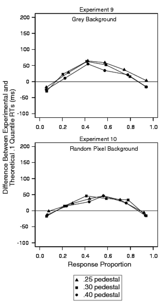
Figure 14 shows the quantile probability functions for the two experiments. The points for the different pedestal contrast conditions fall on the same functions and so are plotted together. The data show small differences in the horizontal and vertical location of the quantiles for each pedestal condition. In each plot, the quantiles are vertically aligned and clustered together for each of the target minus background proportion of white pixels (.5, .1, and .2). The diffusion model fits assumed that only drift rate varied with stimulus contrast and pedestal contrast. The plots show that there is a leading edge effect: The diffusion model fails to predict the .1 quantile in both experiments. Figure 15 shows plots of the difference between the predicted and observed .1 quantiles. It shows that the magnitude of the leading edge effect is similar in magnitude to the earlier experiments with random pixel noise.

Figure 14.

Quantile probability plots for Experiments 9 (letter discrimination with dynamic random pixel noise) with a grey background and Experiment 10 (letter discrimination with dynamic random pixel noise) with a random pixel background.

Figure 15.

Difference between experimental and diffusion model fit for the .1 quantile RTs for Experiments 9 (letter discrimination with dynamic random pixel noise) with a grey background and Experiment 10 (letter discrimination with dynamic random pixel noise) with a random pixel background.

These results showed that, as before, the contrast of the stimulus with the pedestal had a large effect on performance. However, the effect of the contrast of the pedestal with the background was relatively small: at most .04 in accuracy and 27 ms in mean RT. Thus, in this discrimination task, localizing the stimulus with a pedestal does not eliminate the leading edge effect. This is in contrast to the experiments reported by Smith and Ratcliff (2009). In their experiments, the combination of static presentation and a noiseless pedestal eliminated the effect. In Experiments 9 and 10, which used a combination of dynamic noise and a pedestal, the leading edge effect was preserved.

Although the reason for the difference between the two sets of results has yet to be fully identified, we attribute it to our use of dynamic noise in conjunction with a pedestal. In the model of Smith and Ratcliff (2009) evidence begins to accumulate in the decision process as soon a stable VSTM representation of the stimulus begins to form, and the leading edge of the distribution is a measure of the rate of VSTM formation. In the signal detection experiments analyzed by Smith and Ratcliff, which used low contrast grating patches as stimuli, it is likely that the primary determinant of the rate of VSTM formation was the energy content of the stimulus, which was a function of whether or not a pedestal was used. In Experiments 9 and 10, it is likely that the primary determinant of VSTM formation was the time required to extract a stable representation of the stimulus features from a background of dynamic noise. Under these circumstances, any VSTM selection advantage associated with the use of a pedestal would have been lost, and the leading edge effect found with other dynamic noise experiments would be obtained. This is what our Experiments 9 and 10 show.

Experiment 11: Brief presentation of a common line segment

We have shown that, when a letter is embedded in dynamic noise, the diffusion model fails to predict the leading edge of the RT distribution in the most difficult stimulus conditions. This may be because noisy, low-discriminability stimuli provide no signal to the decision process that a stimulus has been presented until after it has been integrated perceptually over several frames. To test this hypothesis, in Experiment 11, a high-contrast luminance signal that was nonpredictive of stimulus identity was presented in the first three frames. To do this, we used letter pairs that shared a common line segment as stimuli and increased the luminance of this segment for the first three frames. If the effect of this signal is sufficient to initiate the decision process, it should reduce mean RT and eliminate or reduce the leading edge effect. Like the pedestal experiments, the purpose of this manipulation was to mark the onset of the stimulus by a burst of contrast energy. Unlike the pedestal experiments, the energy burst was carried by a feature of the stimulus, rather than by its local surround.

Method

The letter pairs used for the experiment were Z-T, R-G, L-P, S-B, N-E, and G-U. They were presented in a Vera Mono 48-point TTF font in a 120×120 random pixel square on a 1280×960 pixel gray background. The random pixel patch was 3.0 by 3.0 cm square and subtended a visual angle of 3.0 degrees at an average viewing distance of 57 cm. On average, there were 350 pixels in a letter; the largest letters were 26 pixels wide and 35 pixels high. As in previous experiments, the stimuli were white letters on a black background. Discriminability was manipulated by inverting .375, .425, .450, or .475 of the pixels. On average, the common segment contained 108 pixels. This segment was presented for three frames at a frame rate of 16.67 ms per frame. The proportion of inverted pixels in the common segment was .150. The brightened common segment was presented on half of the trials and omitted from the other half, in random order. Data were collected from 16 subjects.

Examples of the stimuli are shown in Figure 13 (panels G to J). Figure 13G shows one frame of the letter Z with the horizontal top segment brightened; Figure 13H shows a Z without the brightened segment. Figures 13I and 13J show, respectively, three-frame and seven-frame averages with the horizontal segment brightened for the first three frames.

Results

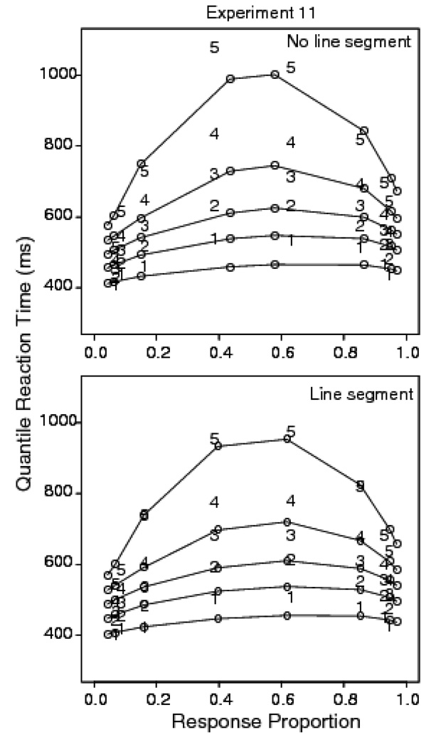
Trials with RTs longer than 2500 ms or shorter than 270 ms were discarded (less than 0.8% of the data, .7% were fast responses). For the no-segment condition, accuracy values for the .375, .425, .450, or .475 inversion conditions were .94, .93, .86, and .59, respectively; the corresponding mean RTs were 528, 572, 648, and 754 ms. For the segment condition, the accuracy values were .375, .425, .450, and .475 and the mean RTs were 524, 561, 634, and 719 ms. The presence of the brightened segment had a small but significant effect on mean RT. There was a 22 ms difference in the leading edge and a 14 ms difference in the mean. The average difference across subjects was significant by paired t-tests for both the .1 quantile, t(15)=9.4, p<.05, and the mean, t(15)=2.73, p<.05.

Figure 16 shows the quantile probability functions for the no-segment and segment conditions. Both show a large leading edge effect. Figure 17 shows the difference in the observed .1 quantiles and the diffusion model predictions. The standard errors of the difference in the .1 quantile in the easiest and most difficult discriminability conditions are 13 ms for the segment condition and 12 ms for the no-segment condition. The corresponding differences in the .1 quantiles are 61 ms and 82 ms, respectively, so the miss is significant. These results show that the presence of the brightened segment reduced the leading edge effect slightly but did not eliminate it.

Figure 16.

Quantile probability plots for Experiment 11 for letter discrimination with random pixel noise and no brightened line segment (top panel) and a brightened line segment for three 16.67 ms frames.

Figure 17.

Difference between experimental and diffusion model fit for the .1 quantile RTs for Experiment 11 for letter discrimination with random pixel noise and no brightened line segment (top panel) and a brightened line segment for three 16.67 ms frames.

Experiment 12: Letter digit discrimination

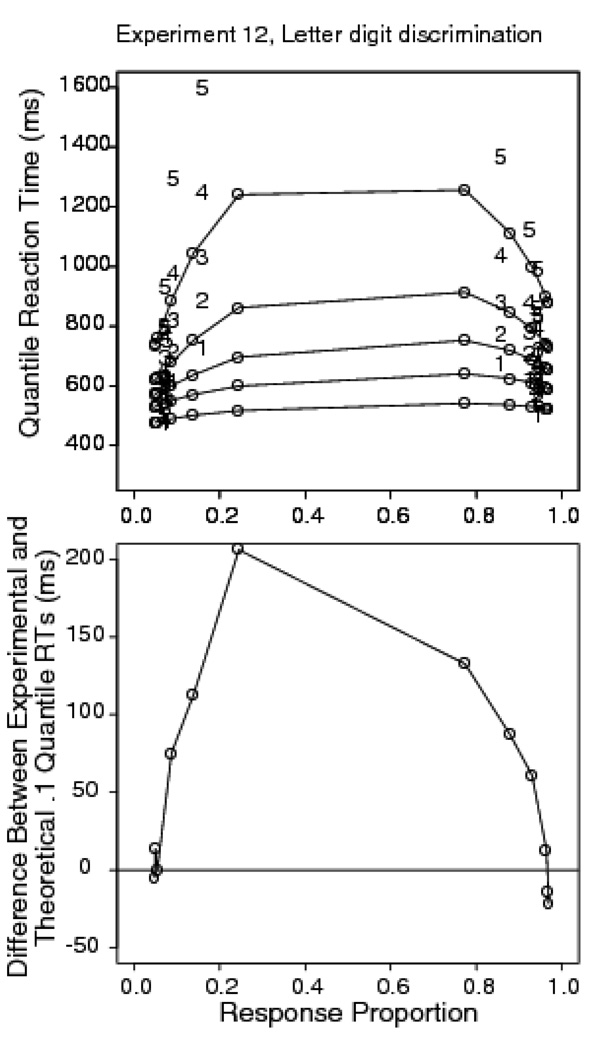
All of the experiments presented so far have involved discrimination between two known perceptual targets: either two target letters that are physically present on the screen; a bright or a dark pixel array, or a rightward or leftward pattern of moving dots. This means that a decision can be based on any perceptual feature that distinguishes between stimuli. In the case of letter discrimination with random pixel noise, it seems that additional time is required to detect the stimulus features when the proportion of inverted pixels is high. Experiment 12 sought to make this component of the task more difficult by using a letter/digit discrimination judgment. Because the set of stimulus alternatives is large, there is no simple perceptual feature that allows letters to be distinguished from digits. Experiment 12 used dynamic noise like that in Experiment 1.

Method

Stimuli were white letters or digits on a black background with some proportion of the pixels inverted. A different sample of pixels was inverted in each 10 ms frame to produce dynamic noise. The proportions of inverted pixels were .25, .30, .35, .39, .41, and .43. Initially, we attempted to select a range of stimulus discriminabilities to span an accuracy range of .6 to .95, as in previous experiments. However, at low levels of accuracy subjects adopted a guessing strategy. This meant that RT did not increase with decreasing discriminability and even decreased in the most difficult condition. We therefore reduced the range of discriminabilities to encourage the subjects to perform the task properly. The letters used as stimuli were F, Q, U, K, N, X, G, L, and R; the digits were 1 through 9. Data were collected from 17 subjects.

Results

Trials with RTs longer than 3000 ms or shorter than 270 ms were discarded (less than 0.8% of the data, .2% were fast responses). Accuracy values for the .25, .30, .35, .39, .41, and .43 inversion conditions were .94, .94, .93, .94, .92, and .85, respectively; the corresponding mean correct RTs were 637, 641, 672, 755, 827, and 948 ms.

The upper panel of Figure 18 shows the quantile probability functions; the lower panel shows the discrepancy between the .1 quantile and the predictions of the diffusion model. There is a very large leading edge effect that the diffusion model is unable to capture. The miss is more than 160 ms for correct responses and more than 200 ms for errors in the most difficult condition. The standard error of the difference in the .1 quantile for the easiest and most difficult conditions was 8 ms, so the miss is very substantial. If we assume the leading edge is a measure of when the decision process begins to accumulate evidence, the data imply that increasing uncertainty about the stimulus significantly increases the delay before accumulation begins. Discriminating among more uncertain alternatives presumably requires higher quality perceptual information, so the large leading edge effect found with letter-digit discrimination implies that, relative to discrimination between letter pairs, the onset of evidence accumulation is delayed until later in encoding. The theoretical interest of these results is they show that the leading edge effect is not just a function of the physical properties of the stimulus, but depends on the kind of decision that must be made. This further underscores the point, made earlier, that the onset of evidence accumulation appears to be adaptively coupled to perceptual encoding. Later in this article, we show that the leading edge effect can be modeled as a delay in the onset of accumulation, under the assumption that the decision is made by a diffusion process.

Figure 18.

Quantile probability plot and a plot of the difference between experimental and diffusion model fit for the .1 quantile RTs for Experiment 12, letter digit discrimination with dynamic random pixel noise.

General Discussion

The experiments reported in this article investigated the relationship between perception and perceptual decision making. Our aim in carrying out these experiments was to identify factors that affect the time course of perceptual processing and to investigate the effects of manipulating these factors on RT and accuracy. The theoretical questions that motivated these experiments were: When does perceptual decision making begin? What information in the stimulus is used to initiate the process of making a decision? These questions are fundamental to our understanding of decision making in simple cognitive tasks.

Our main findings from these experiments were our identification of the leading edge effect and characterization of the conditions under which it was found. We have shown that when letter stimuli are degraded by dynamic, random pixel noise, the leading edge of the RT distribution is delayed. Because the leading edge reflects the fastest responses in the distribution, we interpret the shift as a delay in the time at which the decision process begins to accumulate evidence. The theoretical interest of this result is that it highlights the interdependence of perceptual and decision processes in choice RT.

In stage models of RT (McClelland, 1979; Sternberg, 1969), an encoded representation of a stimulus must be formed before a decision can be made. Stage models assume that stimulus encoding is affected by variables that influence stimulus quality, such as intensity or contrast. For example, Shwartz, Pomerantz, and Egeth (1977) showed that stimulus intensity and stimulus similarity have additive effects on mean RT and RT variance. They interpreted this as evidence that similarity affects a stimulus identification stage, whereas intensity affects an encoding stage. These and other similar findings suggest that variables that affect the perceptual quality of a stimulus act independently of, and prior to, the point at which stimulus information becomes available to the decision process.

Our results are consistent with the stage model view, but go beyond it in showing that only some ways of degrading the stimulus produce a leading edge effect. A large (100 ms or more) leading edge effect was found when stimulus letters are degraded by dynamic, pixel noise (Experiments 1, 8 and 11). A smaller (50 ms) effect was found with static noise (Experiments 3 and 7). When uncertainty about the stimulus alternatives was increased, in the letter-digit discrimination task, the magnitude of the leading edge effect increases to around 150–200 ms (Experiment 12). Critically, the effect is only found in the letter discrimination task. In brightness discrimination there is no leading edge effect with either static or dynamic noise (Experiments 3, 5, and 8). There is no leading edge effect when a letter stimulus is masked by a static array of letter fragments (Experiment 8), or when it is followed by a backward mask (Experiment 4). There is also no leading edge effect in a coherent motion discrimination task when the motion stimulus is degraded by simultaneous, random dot motion (Experiment 6). We also showed that the presence of a localized energy change like a pedestal does not abolish the leading edge effect (Experiments 9 and 10). Nor is it abolished by the presence of an uninformative, high-contrast line segment coinciding with stimulus onset (Experiment 11).

Our data suggest that the leading edge effect arises when noise slows the process of forming a perceptual representation of the stimulus features needed to perform the task. The effect is especially pronounced when the noise is dynamic. When no representation of stimulus features was required, as in the brightness discrimination task, no leading edge effect was found. This is consistent with the experience of doing the task. When one is viewing a letter stimulus, the time needed to perceive it clearly increases with increasing noise. When the level of noise is low, the stimulus seems to become visible almost instantaneously; when the level of noise is high, it seems to become visible only gradually. In the absence of visible stimulus features, there is no perceptual experience of this kind.

The leading edge effect is not simply a general stimulus degradation effect, as degrading letter stimuli with a mask composed of random letter fragments produces no change in the leading edge. Nor is it simply a function of a need to integrate stimulus information over multiple frames, as there is no leading edge effect when discriminating dynamic motion stimuli. Moreover, it is not because noise causes subjects to miss the onset of the stimulus, because marking stimulus onset clearly, either with a pedestal or with an uninformative common feature, does not eliminate the leading edge effect. We are thus left with the conclusion that noise slows the process of forming a representation of the stimulus features, and that the onset of evidence accumulation is tightly coupled to this process.

We quantified the leading edge effect by fitting RT distributions and accuracy with the diffusion model. This model assumes that the time at which the decision process begins to accumulate evidence is independent of the perceptual properties of the stimulus. It also assumes that once the decision process is turned on, the rate of accumulation remains constant across time until a decision is made. This is true even with very brief stimulus presentations (Ratcliff & Rouder, 2000; Smith et al., 2004; Thapar et al., 2003). If mean drift rate is the only model parameter that varies across conditions, the model predicts only small changes in the leading edge of the RT distribution. Other models based on racing diffusion processes (Usher & McClelland, 2001; Ratcliff, Hasegawa, Hasegawa, Smith, & Segraves, 2007) predict the same thing. In most of the experimental paradigms to which the diffusion model has been applied, the change in the leading edge has been small and in agreement with diffusion model predictions. Here, however, we have shown that when letters are degraded by random pixel noise, the change in the leading edge as a function of discriminability is much larger than the diffusion model can predict.

The model fits shown in Figures 4 through 18 were all based on the assumption that the time at which at the decision process is turned on is independent of stimulus quality. If, instead, it is assumed that the time at which the decision process is turned on varies with stimulus quality, then the model fits well, as illustrated in Figure 19. This figure shows the fit of the diffusion model to Experiment 1 under the assumption that T_er, the nondecision component of processing, increases with increases in the proportion of inverted pixels. In this fit, the estimated values of T_er for the 0.35, 0.4, 0.45, and 0.475 inversion conditions were 460, 494, 560, and 600 ms, respectively. Under these conditions, the predicted and observed RT distributions and accuracy values coincide almost exactly.

Figure 19.

Fit of the diffusion model to the data from Experiment 1, letter discrimination with dynamic random pixel noise.

To show the generality of this finding to all 12 experiments, Table 1 presents fit statistics for models in which a single value of T_er was used for all conditions and for models in which T_er was allowed to vary freely across conditions. The chi-squares in the table are based on group data, so they cannot properly be used as absolute measures of fit. Therefore we do not report p values for them. Instead, we focus on the proportional change in fit with changes in the constraints on T_er. As noted earlier, parameters of the diffusion model estimates from group data agree fairly well with the average of the parameters estimated from individual subjects, so there is no evidence that the picture is distorted by fitting group data.

Table 1.

Experiment summary

Experiment and discrimination task	χ2 with one Ter for all conditions	χ2 with one Ter per condition	Leading edge effect
1, dynamic letter discrimination	3389.2	534.1	Yes
2, dynamic brightness discrimination	117.1	114.0	No
3, static letter discrimination	372.5	202.6	Yes
4, masked letter discrimination	69.8	61.4	No
5, masked brightness discrimination	978.3	788.1	No
6, motion discrimination (random dot motion stimuli)	245.6	225.9	No
7, static letter discrimination	492.3	118.5	Yes
7, static brightness discrimination	122.4	120.7	No
8, static letter discrimination	521.6	151.0	Yes
8, dynamic letter discrimination	655.4	223.4	Yes
8, masked letter discrimination	266.5	174.1	No
9, letter discrimination, pedestal, grey	1648.3	498.0	Yes
10, letter discrimination, pedestal, random pixel	1142.1	417.7	Yes
11, letter discrimination, dynamic, no line segment	1149.2	223.3	Yes
11, letter discrimination, dynamic, line segment	680.8	183.7	Yes
12, dynamic letter/digit discrimination	4489.4	729.3	Yes

Note. In the experiments that have more than one line, the different conditions are mixed in the experiment.

In Table 1, the last column lists the experiments in which the plots show a large shift in the leading edge. These experiments should show the largest improvement when T_er is allowed to vary freely across conditions. This pattern was found in all experiments, with two exceptions. In Experiment 8, masked letter discrimination showed a small-to-moderate change in the leading edge in one condition (see Figure 12), which is associated with a 35% change in chi-square. In Experiment 3, letter discrimination in static noise showed a relatively small change in the leading edge and a 44% change in chi-square (see Figure 5). All other experiments showed the expected pattern of a large change in chi-square or a small change in chi-square. The results in Table 1 show that, in general, data from experiments in which there is a leading edge effect are well described by a diffusion model with a variable delay in the onset of evidence accumulation across conditions. Gould (2004) reported a similar result for the leading edge effect in the Gould et al. (2007) experiment analyzed by Smith and Ratcliff (2009).

As noted in the introduction, a criticism sometimes made of diffusion models is that they are so flexible that they could fit any conceivable pattern of data. Ratcliff (2002) showed that this was not so and argued, rather, that the diffusion model predicts a limited and tightly-constrained set of distributions which are precisely those found in empirical data. Figure 20 presents further evidence that bears upon this point. The figure shows plots of the quantile RTs for correct responses for each experiment as a function of the quantile RTs for the most accurate condition in the experiment. If the shape of the distributions is invariant across conditions, the quantile-quantile plots will be linear. The plots in Figure 20 show that, to a good approximation, this is indeed the case. The same invariance is shown by the distributions predicted by the diffusion model (Ratcliff & McKoon, 2008).

Figure 20.

Plots of quantile RTs against quantile RTs for correct responses for all the experiments. Experiment 5 has only half the conditions plotted. In each case, the quantiles for the less accurate conditions are plotted against the quantiles for the most accurate condition.

Invariance of distribution shape is one of the most powerful constraints on models of RT distributions. A successful model must predict this invariance across all conditions in an experiment, in which accuracy can vary from near chance to near perfect. Invariance is not a property of atheoretical families like the ex-Gaussian and the Weibull, which encompass a wide range of shapes, including symmetric distributions and extremely skewed distributions. In contrast to this, the degree of distributional invariance in our experiments is striking, given the variety of different stimulus configurations we used. That the diffusion model predicts this invariance is a strong argument in support of its use in performing process decomposition of RT data.

The theoretical problem posed by our results is in understanding precisely how the onset of evidence accumulation in the decision process is initiated by the encoding of the stimulus. If the decision process were turned on at the same time for each stimulus type, there would be only a small change in the leading edge of the RT distribution. This is exactly the pattern shown in Experiment 5 (masked brightness discrimination). In the most difficult conditions, accuracy is near chance (.5) and the estimated drift rate is near zero. Under these conditions, the process is accumulating mainly noise. Nevertheless, there is only a small change in the leading edge, because the fastest-finishing processes reach a decision criterion quickly due to the noisiness of the process. The amount of noise needed to fit the RT distributions means that a change from a large to a zero or near-zero drift rate produces only a small change in the leading edge.

Another possibility we can exclude is that subjects use different decision criteria for different stimuli. Suppose subjects were able to make some kind of assessment of the properties of the stimulus at the beginning of a trial and to use this to adjust their decision criteria. This might lead them to set higher criteria for more difficult stimuli. Although this would change mean RT, it would have only a small effect on the fastest finishing processes, at least for plausible values of the criteria. Large changes in criteria can predict large changes in the leading edge, but only at the expense of also predicting changes in the slowest responses (the .9 quantile) that far exceed those found in data. We are thus left with the idea that the time at which the decision process begins to accumulate evidence depends on the properties of the stimulus.

We can think of two mechanisms that could provide the required coupling between stimulus encoding and evidence accumulation. These two mechanisms have features in common with the discrete-stage and continuous-flow models described in the processing stages literature. The first was proposed by Smith and Ratcliff (2009). In their model, the output of visual filters that encode the stimulus are transferred to VSTM under the control of spatial attention. The model assumes that the drift of the diffusion process is proportional to the strength of the VSTM trace. Like the cascade model of McClelland (1979), the model assumes that the decision process begins to accumulate evidence as soon as encoded stimulus information begins to become available. To provide the required coupling between encoding and evidence accumulation, the model assumes that the within-trial variance in the VSTM trace grows in proportion to mean trace strength. Prior to stimulus presentation, the mean and the variance of the VSTM trace are both zero, so there is no evidence accumulation. Accumulation begins only when the trace mean and moment-to-moment variance both change from zero. Smith and Ratcliff showed that this model satisfactorily described the leading edge effect (approximately 50 ms) in the data of Gould et al. (2007), in which low contrast sinusoidal grating patches were briefly flashed for 40 ms on a uniform field.

The second, more physiologically motivated, mechanism assumes that evidence accumulation is suppressed, or inhibited, prior to stimulus presentation. Variability in the signal will also be suppressed so that it is small and will not lead to threshold crossing. At some point, when stimulus encoding is complete, the inhibition is released. The effect of release from inhibition is to allow diffusive accumulation of information (both signal and noise) to begin. Release from inhibition could be controlled by some global measure of the quality of the stimulus representation and could occur when this measure reaches a threshold. In its assumption of a single, threshold-dependent signal which produces a step change in the accumulation process, this mechanism is similar to the discrete stages models in the processing stages literature.

One way to realize a release from inhibition mechanism computationally is with an Ornstein-Uhlenbeck diffusion process (Busemeyer & Townsend, 1992; Smith, 1995). Unlike the Wiener diffusion process in Ratcliff’s (1978) model, which we fitted here, the Ornstein-Uhlenbeck process is a diffusion process with decay. The effect of decay is to constrain the value of the accumulated evidence to remain near zero. This is best understood in terms of the paths that describe the accumulating evidence on individual trials, as shown in Figure 1 (the so-called "sample paths" of the diffusion process). When decay in the Ornstein-Uhlenbeck is large, with high probability, most of the sample paths stay in a small region surrounding the starting point. They are thus unlikely to cross a decision boundary and produce a response. When decay is small, the paths fan out and become more variable, and so are more likely to cross a boundary and produce a response.

Release from inhibition could therefore be represented as a change from a large to a small value of Ornstein-Uhlenbeck decay, initiated by the completion of stimulus encoding. Ratcliff et al. (2007) discussed neurophysiological evidence for modulation of the evidence accumulation process by generalized inhibition. Unlike the continuous-flow model of Smith and Ratcliff (2009), in which diffusive evidence accumulation begins automatically as soon as stimulus information begins to enter VSTM, the release from inhibition account requires an additional mechanism to initiate evidence accumulation, possible when the quality of the stimulus encoding reaches some threshold.

Both of the mechanisms we have proposed assume that the effect of presenting a letter target in noise is to slow the perceptual encoding of a stimulus, and that the time course of evidence accumulation is adaptively coupled to the time course of encoding. What is the mechanism that leads to this slowing of encoding? We cannot give a definitive answer to this question, but we think it probably reflects competitive interactions among filters in the early visual system that are tuned to different spatial scales and orientations. Presenting a stimulus in random pixel noise activates a random sample of visual filters that are tuned to scales and orientations other than those that carry information about the target stimulus. Competitive interactions among these filters may slow the processing of stimulus information by the filters that code the target and lead to the perceptual experience of a slowly emerging stimulus.

This still leaves unresolved the problem of the large leading edge effect obtained with dynamic noise. As well as reducing stimulus contrast, increasing the proportion of inverted pixels in a dynamic display reduces the frame-to-frame correlation in the stimulus. A plausible hypothesis for the dynamic noise case is that the rate of perceptual encoding is a function of the space- averaged, temporal correlation in the stimulus. This correlation can be viewed as a measure of the temporal stability or temporal persistence in the stimulus. When the correlation is high, encoding is rapid; when the correlation is low, encoding is slow.

Figure 21 shows in schematic form a simple neural mechanism that could underlie this effect. Stimulus features are encoded by oriented receptive fields, assumed to possess similar properties to receptive fields in visual area V1. At any time, t, the evidence for the presence of a feature at that location is reflected in the activity in a population of "collector neurons." Each of these neurons has a set of random delay lines as its afferents. At any time, t, one of these afferents codes the presence of a feature at that location at some prior time, t - h. The entire set of afferents codes the presence of the feature over a range of times, t - h, t - 2h, t - 3h, and so on. The neuron will fire only if the feature is present in some threshold number of the preceding time slices. The higher the temporal correlation in the stimulus, the more likely this is to occur. We assume that the rate of perceptual encoding is a function of the firing rates in such neurons.

Figure 21.

Delay line coding model. Activity in a random pixel array is coded by oriented receptive fields. Collector neurons receive inputs via delay lines from time slices t - h, t - 2h, t - 3h, etc. The neurons fire at time t only if the sum of their inputs exceeds a threshold. Delay line coding detects the presence of persistent structure in the stimulus while suppressing transient structure. In the example, the two collector neurons receive inputs from receptive fields that detect the crossbar and the upright of a capital T, respectively. This coding scheme also produces spatiotemporal summation. Features can be detected even when degraded (represented here by one of the three locations in the receptive field left unfilled) in the presence of temporal correlation in the input. In this example, if the two collector neurons have a threshold of 7 units of input, both will fire in response to the three stimulus frames shown. The model assumes that the rate of neural firing determines the rate at which a stable perceptual representation of the stimulus is formed.

The coding scheme in Figure 21 makes sense biologically because it detects persistent structure in the stimulus while suppressing transients. Because the latter are more likely to have arisen through noise, the effect of such random delay line encoding is to yield a cleaned up representation of the stimulus. In most situations such a representation will be biologically adaptive.

One of the implications of this account is that any manipulation that perturbs the temporal structure of the stimulus, not just random pixel noise, should produce a leading edge effect. That this is so was shown by Yap, Balota, Tse, and Besner (2008). They showed, by means of an ex- Gaussian analysis of RT distributions, that word frequency and stimulus quality had additive effects on RT in a lexical decision task. They manipulated stimulus quality using a noise mask, which they created by presenting words and strings of masking characters in alternating video frames. Like Shwartz et al. (1977), they interpreted distributional additivity as evidence for a discrete stage model, in which stimulus quality affects perceptual encoding and word frequency affects lexical retrieval (i.e., stimulus identification and decision making). For us, the significance of Yap et al’s findings is that they showed that the presence of random, transient visual structure also results in a leading edge effect.

Conclusion

In this article we have investigated a question that has its origins in the literature on stage models of RT. This is the question of how the occurrence of a new stimulus initiates the process of making a decision. The success of models like the diffusion model in accounting for the detailed properties of RT distributions and response accuracy in choice RT tasks has often meant that the significance of this theoretical problem has been ignored. (The work of Laming, 1968, is a notable exception to this.) This is particularly so in the context of laboratory studies of choice RT, which typically present known stimulus alternatives at predictable times in predictable locations. Under these circumstances, it is not always obvious that the problem of understanding how a new stimulus initiates a decision is almost as fundamental as that of understanding how the decision itself is made.

The problem of how decisions are initiated is thrown into sharp relief by considering decision making in everyday life. Our everyday perceptual experience does not have the discrete trial structure of a laboratory task. Rather, our experience is one of continuous perceptual flux, in which novel stimuli appear at unexpected times and at unexpected locations. Indeed, the stimuli to which we must respond can appear in any sensory modality, not just vision. While driving, or walking, or in conversation, we constantly make decisions and initiate actions, in response to the requirements of the situation. Not only must we decide on what responses to make in such situations, we must also decide on the appropriate modality to make them in: vocally, or manually, with eyes, hands, feet, or whole of body. Because of the complexity of the environment in which the human perception-action system evolved, it must be able to switch among these alternatives rapidly and with relatively little cost. We view the decision process as one that can take its inputs from any one of a number of sources, either externally, from any sensory modality, or internally, from knowledge stored in memory, and which can both select an appropriate response and an appropriate response modality to express it in. The decision process might be centrally located or the evidence might be funneled to more peripheral locations that implement the evidence accumulation process (e.g., Ratcliff et al., 2007).

The experiments described in this article do not provide a final answer to this question, which we believe to be a complex one. However, they illustrate in an extremely graphic way the interdependence between perceptual and decision processes. We have shown that manipulations that affect the time course of perceptual processing also affect the time course of decision making, and, in particular, the time at which decisions are initiated. We have shown that these effects are not simply strategic adaptations to the demands of the task, but reflect something more fundamental about the coupling of perception and decision making. They are not simply a feature of task difficulty, but are specific to the requirement to process particular kinds of perceptual information. We have suggested two plausible mechanisms whereby the coupling between perceptual and decision processes could be effected, and we have presented a new experimental paradigm, which we believe will be a useful tool to investigate these mechanisms in future.

References

- Busemeyer JR, Townsend JT. Fundamental derivations from decision field theory. Mathematical Social Sciences. 1992;23:255–282. [Google Scholar]
- Donders FC. On the speed of mental processes. In: Koster WG, translator; Koster WG, editor. Attention and Performance II. Amsterdam: North-Holland: 1969. pp. 412–431. (Original work published in Onderzoekingen Gedann in het Psycologisch Laboratorium der Utrechtsche Hoogeschool, Tweede reeks, 1868–1869, II, pp. 92–120.). [Google Scholar]
- Gomez P, Ratcliff R, Perea M. A model of the go/no-go task. Journal of Experimental Psychology: General. 2007;136:347–369. doi: 10.1037/0096-3445.136.3.389. [DOI] [PMC free article] [PubMed] [Google Scholar]
- Gould IC. Unpublished B.Sc. Honors thesis. The University of Melbourne; 2004. Attentional mechanisms in visual signal detection: Signal enhancement or uncertainty reduction. [Google Scholar]
- Gould IC, Wolfgang BJ, Smith PL. Spatial uncertainty explains endogenous and exogenous cuing effects in visual signal detection. Journal of Vision. 2007;7:1–17. doi: 10.1167/7.13.4. [DOI] [PubMed] [Google Scholar]
- Hohle RH. Inferred components of reaction times as a function of foreperiod duration. Journal of Experimental Psychology. 1965;69:382–386. doi: 10.1037/h0021740. [DOI] [PubMed] [Google Scholar]
- Laming DRJ. Information theory of choice reaction time. New York: Wiley; 1968. [Google Scholar]
- McClelland J. On the time relations of mental processes: An examination of systems of processes in cascade. Psychological Review. 1979;86:287–330. [Google Scholar]
- Nelder JA, Mead R. A simplex method for function minimization. Computer Journal. 1965;7:308–313. [Google Scholar]
- Ratcliff R. A theory of memory retrieval. Psychological Review. 1978;85:59–108. [Google Scholar]
- Ratcliff R. Continuous versus discrete information processing: Modeling the accumulation of partial information. Psychological Review. 1988;95:238–255. doi: 10.1037/0033-295x.95.2.238. [DOI] [PubMed] [Google Scholar]
- Ratcliff R. Putting noise into neurophysiological models of simple decision making (letter) Nature Neuroscience. 2001;4:336. doi: 10.1038/85956. [DOI] [PubMed] [Google Scholar]
- Ratcliff R. A diffusion model account of reaction time and accuracy in a two choice brightness discrimination task: Fitting real data and failing to fit fake but plausible data. Psychonomic Bulletin and Review. 2002;9:278–291. doi: 10.3758/bf03196283. [DOI] [PubMed] [Google Scholar]
- Ratcliff R. Modeling Response Signal and Response Time Data. Cognitive Psychology. 2006;53:195–237. doi: 10.1016/j.cogpsych.2005.10.002. [DOI] [PMC free article] [PubMed] [Google Scholar]
- Ratcliff R. The EZ diffusion method: Too EZ? Psychonomic Bulletin and Review. 2008;15:1218–1228. doi: 10.3758/PBR.15.6.1218. [DOI] [PMC free article] [PubMed] [Google Scholar]
- Ratcliff R, Gomez P, McKoon G. A diffusion model account of the lexical-decision task. Psychological Review. 2004;111:159–182. doi: 10.1037/0033-295X.111.1.159. [DOI] [PMC free article] [PubMed] [Google Scholar]
- Ratcliff R, Hasegawa YT, Hasegawa YP, Smith PL, Segraves MA. Dual diffusion model for single-cell recording data from the superior colliculus in a brightness- discrimination task. Journal of Neurophysiology. 2007;97:1756–1774. doi: 10.1152/jn.00393.2006. [DOI] [PMC free article] [PubMed] [Google Scholar]
- Ratcliff R, McKoon G. The diffusion decision model: Theory and data for two-choice decision tasks. Neural Computation. 2008;20:873–922. doi: 10.1162/neco.2008.12-06-420. [DOI] [PMC free article] [PubMed] [Google Scholar]
- Ratcliff R, Murdock BB., Jr Retrieval processes in recognition memory. Psychological Review. 1976;83:190–214. [Google Scholar]
- Ratcliff R, Rouder JN. Modeling Response Times for Two-Choice Decisions. Psychological Science. 1998;9:347–356. [Google Scholar]
- Ratcliff R, Rouder JN. A diffusion model account of masking in letter identification. Journal of Experimental Psychology: Human Perception and Performance. 2000;26:127–140. doi: 10.1037//0096-1523.26.1.127. [DOI] [PubMed] [Google Scholar]
- Ratcliff R, Smith PL. A comparison of sequential sampling models for two-choice reaction time. Psychological Review. 2004;111:333–367. doi: 10.1037/0033-295X.111.2.333. [DOI] [PMC free article] [PubMed] [Google Scholar]
- Ratcliff R, Thapar A, Gomez P, McKoon G. A diffusion model analysis of the effects of aging in the lexical-decision task. Psychology and Aging. 2004;19:278–289. doi: 10.1037/0882-7974.19.2.278. [DOI] [PMC free article] [PubMed] [Google Scholar]
- Ratcliff R, Thapar A, McKoon G. The effects of aging on reaction time in a signal detection task. Psychology and Aging. 2001;16:323–341. [PubMed] [Google Scholar]
- Ratcliff R, Thapar A, McKoon G. A diffusion model analysis of the effects of aging on brightness discrimination. Perception and Psychophysics. 2003;65:523–535. doi: 10.3758/bf03194580. [DOI] [PMC free article] [PubMed] [Google Scholar]
- Ratcliff R, Thapar A, McKoon G. A diffusion model analysis of the effects of aging on recognition memory. Journal of Memory and Language. 2004;50:408–424. [Google Scholar]
- Ratcliff R, Thapar A, McKoon G. Aging and individual differences in rapid two- choice decisions. Psychonomic Bulletin and Review. 2006;13:626–635. doi: 10.3758/bf03193973. [DOI] [PMC free article] [PubMed] [Google Scholar]
- Ratcliff R, Tuerlinckx F. Estimating the parameters of the diffusion model: Approaches to dealing with contaminant reaction times and parameter variability. Psychonomic Bulletin and Review. 2002;9:438–481. doi: 10.3758/bf03196302. [DOI] [PMC free article] [PubMed] [Google Scholar]
- Ratcliff R, Van Zandt T, McKoon G. Connectionist and diffusion models of reaction time. Psychological Review. 1999;106:261–300. doi: 10.1037/0033-295x.106.2.261. [DOI] [PubMed] [Google Scholar]
- Rouder JN, Tuerlinckx F, Speckman PL, Lu J, Gomez P. A hierarchical approach for fitting curves to response time measurements. Psychonomic Bulletin & Review. 2008;15:1201–1208. doi: 10.3758/PBR.15.6.1201. [DOI] [PubMed] [Google Scholar]
- Schweickert R. A critical path generalization of the additive factor method: Analysis of a Sroop task. Journal of Mathematical Psychology. 1978;18:105–139. [Google Scholar]
- Shwartz SP, Pomerantz JR, Egeth HE. State and process limitations in information processing: An additive factors analysis. Journal of Experimental Psychology: Human Perception and Performance. 1977;3:402–410. [Google Scholar]
- Smith PL. Psychophysically principled models of visual simple reaction time. Psychological Review. 1995;102:567–591. [Google Scholar]
- Smith PL. Stochastic dynamic models of response time and accuracy: A foundational primer. Journal of Mathematical Psychology. 2000;44:408–463. doi: 10.1006/jmps.1999.1260. [DOI] [PubMed] [Google Scholar]
- Smith PL, Ratcliff R. An Integrated Theory of Attention and Decision Making in Visual Signal Detection. Psychological Review. 2009;116:283–316. doi: 10.1037/a0015156. [DOI] [PubMed] [Google Scholar]
- Smith PL, Ratcliff R, Wolfgang BJ. Attention orienting and the time course of perceptual decisions: response time distributions with masked and unmasked displays. Vision Research. 2004;44:1297–1320. doi: 10.1016/j.visres.2004.01.002. [DOI] [PubMed] [Google Scholar]
- Sternberg S. The discovery of processing stages: Extensions of Donder’s method. In: Koster WG, editor. Attention and performance II. Amsterdam: North-Holland: 1969. pp. 276–315. [Google Scholar]
- Thapar A, Ratcliff R, McKoon G. A diffusion model analysis of the effects of aging on letter discrimination. Psychology and Aging. 2003;18:415–429. doi: 10.1037/0882-7974.18.3.415. [DOI] [PMC free article] [PubMed] [Google Scholar]
- Usher M, McClelland JL. The time course of perceptual choice: The leaky, competing accumulator model. Psychological Review. 2001;108:550–592. doi: 10.1037/0033-295x.108.3.550. [DOI] [PubMed] [Google Scholar]
- Vickers D. An adaptive module of simple judgements. In: Requin J, editor. Attention and Performance, VII. Hillsdale, N.J: Erlbaum; 1978. pp. 599–618. [Google Scholar]
- Voss A, Rothermund K, Voss J. Interpreting the parameters of the diffusion model: An empirical validation. Memory and Cognition. 2004;32:1206–1220. doi: 10.3758/bf03196893. [DOI] [PubMed] [Google Scholar]
- Wagenmakers E-J, Ratcliff R, Gomez P, McKoon G. A diffusion model account of criterion shifts in the lexical decision task. Journal of Memory and Language. 2008;58:140–159. doi: 10.1016/j.jml.2007.04.006. [DOI] [PMC free article] [PubMed] [Google Scholar]
- Yap MJ, Balota DA, Tse C-S, Besner D. On the additive effects of stimulus quality and word frequency in lexical decision: Evidence for opposing interactive influences revealed by RT distributional analyses. Journal of Experimental Psychology: Learning, Memory, and Cognition. 2008;34:495–513. doi: 10.1037/0278-7393.34.3.495. [DOI] [PubMed] [Google Scholar]