PARAMETER ESTIMATION AND DYNAMIC SOURCE LOCALIZATION FOR THE MAGNETOENCEPHALOGRAPHY (MEG) INVERSE PROBLEM

Abstract

Dynamic estimation methods based on linear state-space models have been applied to the inverse problem of magnetoencephalography (MEG), and can improve source localization compared with static methods by incorporating temporal continuity as a constraint. The efficacy of these methods is influenced by how well the state-space model approximates the dynamics of the underlying brain current sources. While some components of the state-space model can be inferred from brain anatomy and knowledge of the MEG instrument noise structure, parameters governing the temporal evolution of underlying current sources are unknown and must be selected on an ad-hoc basis or estimated from data. In this work, we apply the Expectation-Maximization (EM) algorithm to estimate parameters and sources in an MEG state-space model, and demonstrate in simulation studies that the resulting source estimates are superior to those provided by static methods or dynamic methods employing ad hoc parameter selection.

1. INTRODUCTION

Advances in medical imaging over the past several decades have provided researchers with the tools necessary to non-invasively measure human brain function in normal and disease states. Magnetoencephalography (MEG) is one such technique that measures the magnetic fields generated by neuronal currents associated with brain activity [1]. The ill-posed nature of the electromagnetic inverse problem and the relatively large distance between the sensors and the sources restrict the spatial resolution of MEG [1]. However, MEG permits observation of neural events on a time-scale of milliseconds, revealing brain dynamics that cannot be seen with slower imaging modalities such as functional magnetic resonance imaging (fMRI) or positron emission tomography (PET).

Established methods for MEG source imaging, such as the minimum-norm estimate (MNE) [2,3], provide static estimates where each time point is treated independently. Recently, dynamic estimation methods have been applied to electroencephalography (EEG) and MEG data. Galka, et al. [4] used a random walk model with a Laplacian spatial smoothness constraint to represent the dynamics of EEG source currents, and estimated these source currents using the Kalman filter (KF) and recursive least-squares algorithms. Long, et al. [5, 6] proposed a similar random walk model for MEG source currents, and estimated these sources using both the causal KF and the Fixed Interval Smoother (FIS) algorithms. The temporal-continuity constraint introduced by these methods not only improved the estimation of the source time-series, but also resulted in improved spatial localization. Temporal and spatial improvements were greater for the FIS algorithm, due to the fact that the FIS uses the entire data record to estimate the source currents [5, 6].

The efficacy of these dynamic methods is strongly influenced by how well the state-space model approximates the dynamics of the underlying brain current sources. While some components of the state-space model can be inferred from brain anatomy and knowledge of the noise structure of the MEG instrument, parameters governing the temporal evolution of the current sources are unknown and must be selected on an ad-hoc basis or estimated from data. In this work, we apply the Expectation-Maximization (EM) algorithm to estimate parameters and sources in an MEG state-space model, and demonstrate in simulation studies that the resulting source estimates are superior to those provided by static methods or dynamic methods employing ad hoc parameter selection.

2. METHODS

2.1 State-Space Model for MEG

In an MEG experiment, we obtain a recording of the magnetic field from hundreds of sensors located outside the head. For N large, assume that the data are sampled at times tΔ for t = 1,…,N. Let y_s(tΔ) denote the measurement at time tΔ in sensor s, where s = 1,…S. We define y_t = [y₁(tΔ),…,y_S(tΔ)] to be the S × 1 observation vector at time tΔ. We assume that there are M sources. Let x_m(tΔ) denote the cortical source activity at time tΔ at location m, where m = 1,…,M. We define x_t = [x₁(tΔ),…, x_M(tΔ)] as the M × 1 state vector. The relationship between the observations vector and the state vector is given by the observation equation

$$y_t=G{x}_t+v_t,$$ (1)

where G is an S × M lead field matrix computed using a quasistatic approximation of the Maxwell’s equations [1], and v_t is the S × 1 vector of zero mean Gaussian noise with covariance matrix C representing the background machine noise. We assume that x_t follows the spatio-temporal model

$$x_m(t\mathrm{\Delta })=a{x}_m((t-1)\mathrm{\Delta })+b{q}_m^{-1}\sum _{m\in N(m)}{x}_m((t-1)\mathrm{\Delta })+w_t,$$ (2)

similar to that proposed in [4], where a and b are scalars such that a + b = 1, N(m) is the neighborhood of source m, q_m is the number of neighbors of source m, and w_t is a M × 1 zero mean Gaussian noise vector with covariance matrix $Q=\mathit{diag}({\sigma }_1^2,{\sigma }_2^2,\dots ,{\sigma }_M^2)$. We can rewrite Eq. 2 as the multivariate autoregressive model

$$x_t=F{x}_{t-1}+w_t,$$ (3)

where the transition matrix F encompasses the neighborhood interactions between the sources at time t in terms of the sources in the previous time step. The initial value x₀ is assumed to be a Gaussian vector with mean μ and covariance matrix Σ. Equations (1) and (3) define the state-space model for MEG.

2.2 Maximum Likelihood Estimation Using the Expectation-Maximization (EM) algorithm

In the above model, the lead field matrix G can be computed using the boundary-element model based on high-resolution magnetic resonance images (MRI) [7], and the observation noise covariance C can be estimated from empty room recordings. The state transition matrix F can be set to identity (I), or to incorporate local spatial smoothing as in [2]. The remaining unknown parameter is the state (source current) noise covariance matrix Q. In this section we present an EM algorithm for estimating Q. This algorithm makes use of the fact that, under the Gaussian state-space model described in 2.1, the conditional expectations for the E-step of the EM algorithm are provided by the FIS [8].

The joint likelihood of the complete data x₀,…, x_N, y₁,…, y_N can be written in the form

$$\begin{array}{l}logL=-\frac{1}{2}log\mid \mathrm{\sum }\mid -\frac{1}{2}{(x_0-\mu )}^T{\mathrm{\sum }}^{-1}(x_0-\mu )\\ -\frac{N}{2}log\mid Q\mid -\frac{1}{2}\sum _{t=1}^N{(x_t-F{x}_{t-1})}^T{Q}^{-1}(x_t-F{x}_{t-1}),\\ -\frac{N}{2}log\mid C\mid -\frac{1}{2}\sum _{t=1}^N{(y_t-G{x}_t)}^T{C}^{-1}(y_t-G{x}_t)\end{array}$$ (4)

where L is to be maximized with respect to the parameter matrix θ = Q. Since the log likelihood depends on the unobserved time series x_t, t = 1,…,N, the EM algorithm is applied conditionally with respect to the observed series y_t, t = 1,…,N, as demonstrated in [9]

$$G(\theta )=E_r(logL\mid y_1,y_2,\dots ,y_N),$$ (5)

where E_r denotes the conditional expectation relative to the density containing the rth iterate value Q(r). In order to calculate the conditional expectation in Eq. (5), it is convenient to define the conditional mean

$$x_{t\mid N}=E(x_t\mid y_1,y_2,\dots ,y_N),$$ (6)

and covariance functions

$$P_{t\mid N}=cov(x_t\mid y_1,y_2,\dots ,y_N)$$ (7)

$$P_{t,t-1\mid N}=cov(x_t,x_{t-1}\mid y_1,y_2,\dots ,y_N).$$ (8)

Taking conditional expectation in Eq. (4) yields.

$$\begin{array}{l}G(\theta )=-\frac{1}{2}\mid \mathrm{\sum }\mid -\frac{1}{2}tr\left\{{\mathrm{\sum }}^{-1}\left(P_{0\mid N}+\left(x_{0\mid N}-\mu \right){\left(x_{0\mid N}-\mu \right)}^T\right)\right\}\\ -\frac{N}{2}log\mid Q\mid -\frac{1}{2}tr\left\{Q^{-1}(H-D{F}^T-F{D}^T+FB{F}^T)\right\}\\ -\frac{N}{2}log\mid C\mid -\frac{1}{2}tr\left\{C^{-1}\sum _{t=1}^N\left[(y_t-G{x}_{t\mid N}){(y_t-G{x}_{t\mid N})}^T+G{P}_{t\mid N}{G}^T\right]\right\},\end{array}$$ (9)

where

$$B=\sum _{t=1}^N\left(P_{t-1\mid N}+x_{t-1\mid N}{x}_{t-1\mid N}^T\right),$$ (10)

$$D=\sum _{t=1}^N\left(P_{t,t-1\mid N}+x_{t\mid N}{x}_{t-1\mid N}^T\right),\text{and}$$ (11)

$$H=\sum _{t=1}^N\left(P_{t\mid N}+x_{t\mid N}{x}_{t\mid N}^T\right).$$ (12)

Choosing

$${\sigma }_m^2(r+1)=\frac{{[Z]}_{m,m}}{N},$$ (13)

where

$$Z=H-D{F}^T-F{D}^T+FB{F}^T$$ (14)

maximizes line 2 in equation (9). As in [9], the first line in equation (9) is analogous to a single replication of a normal likelihood so that one may take μ(r + 1) = x_0|N and Σ(r + 1) = P_0|N. The estimates x_t|N, Σ_t|N and Σ_t,t−1|N for the rth iterate are computed using the value Q(r + 1), μ(r + 1) and Σ(r + 1) using the FIS [8] and the one-step covariance algorithm [9].

We set the structure of the state transition matrix F in the FIS computation such that a = 0.5 and b = 0.5. We begin by computing a static estimate with the MNE method, x_MNE,t=1, using y₁, the observation noise covariance from the MEG background noise C, and the source covariance R = γI where trace(HRH^T)/trace(C) = 1. Then we compute Σ_MNE = cov(x_MNE). At last, we set μ(0) = x_MNE,t=1, Σ(0) = Σ_MNE, Q(0) = R, and iterate until the log likelihood converges. The value of the log likelihood is calculated using the ‘innovations’ form [10]:

$$\begin{array}{l}logL\equiv -\frac{1}{2}\sum _{t=1}^{N}log\mid G{P}_{t\mid t-1}{G}^T+C\mid \\ -\frac{1}{2}\sum _{t=1}^N{(y_t-G{x}_{t\mid t-1})}^T{(G{P}_{t\mid t-1}{G}^T+C)}^{-1}(y_t-G{x}_{t\mid t-1})\end{array}$$ (15)

2.3 Simulation Studies

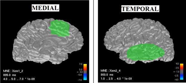
We employed simulation studies to compare source localization performance of the static (MNE), dynamic (FIS), and EM solutions. We constrained the source locations to the cortical mantle with about 6-mm spacing between adjacent sources [3]. We chose regions of interest (ROIs) in the medial surface and the temporal lobe of the left hemisphere as shown in Figure 1. The medial ROI contains 75 sources, while the temporal ROI contains 181 sources. We restricted the dimensionality of the problem to reduce computational complexity, with the rationale that higher-order versions could be implemented later using high-performance computing resources as in [6]. We computed the lead field matrix for sources in the two ROIs with dipole orientations constrained to the normal of the cortical mantle assuming the sensor configuration of the 306-channel Vectorview MEG system (Elekta-Neuromag, Helsinki, Finland) used at our Center.

Figure 1.

Reconstructed cortical surface from structural MRI scans and ROIs.

The time course of the the sources on each ROI was simulated as a 10-Hz sinusoidal oscillation over a period of 1 second in order to emulate a realistic MEG experiment:

$$x_m(t\mathrm{\Delta })=\{\begin{array}{cc}sin(2\pi \ast 10t\mathrm{\Delta })& \text{if}{x}_m\text{is}\text{active}\\ 0& \text{if}{x}_m\text{is}\text{inactive}\end{array},$$ (16)

where the sampling frequency 1/Δ is 200 Hz. The percentage of active sources in both simulations was approximately 20 percent. The observation equation (1) was then used to obtain the simulated MEG recordings. The signal-to-noise ratio (SNR) was set to 5, a value typical for MEG measurements [1], with signal amplitudes scaled uniformly across the active regions to achieve this SNR.

3. RESULTS AND DISCUSION

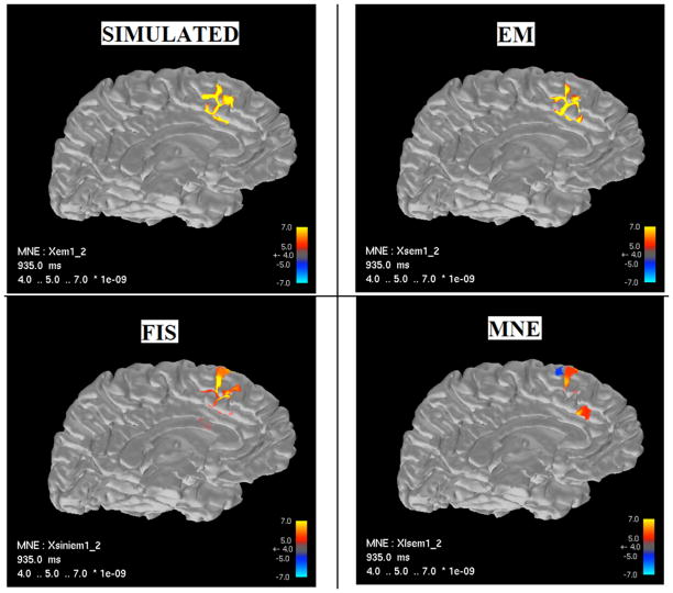
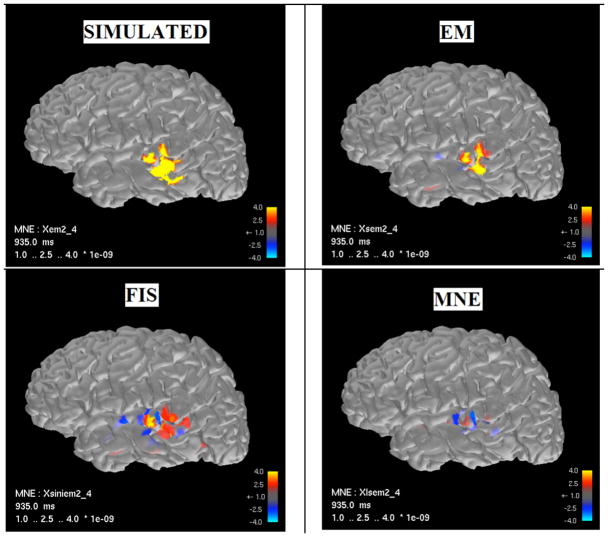
Figures 2 and 3 show the source current estimates for the medial and temporal ROIs, respectively, estimated using the MNE, FIS, and EM algorithms. In both cases, sources estimated using the EM algorithm (upper right) show a much closer correspondence to the true simulated source distribution (upper left) than either the MNE or FIS algorithms (lower right and left, respectively).

Figure 2.

Source localization results from medial ROI.

Figure 3.

Source localization results from temporal ROI.

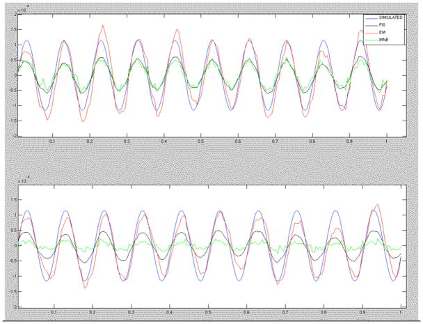
In accordance with Figures 2 and 3, the EM time courses show the closest correspondence to the true source time course. Figure 4 shows the time-course estimates from two representative source locations.

Figure 4.

Comparison of source current time-course estimates. The simulated source is shown in blue, the EM algorithm estimate in red, the FIS estimate in black, and the MNE in green.

4. CONCLUSIONS AND FUTURE WORK

We applied the Expectation-Maximization (EM) algorithm to estimate parameters and sources in an MEG state-space model, and demonstrated in simulation studies that these estimates significantly improve MEG source localization and time-course estimates compared to static or dynamic methods relying on ad hoc parameter selection. These findings highlight the importance of parameter estimation for an accurate state-space representation of the MEG inverse problem. Future studies will examine performance of these methods on experimental data from human subjects, and will employ high-performance computing methods and resources so that the entire cortical surfaces can be analyzed.

References

- 1.Hämäläinen MS, Hari R, Ilmoniemi RJ, Knuutila J, Lounasmaa OV. Magnetoencephalography – theory, instrumentation, and applications to non-invasive studies of the working human brain. Rev Mod Phys. 1993;65:413–497. [Google Scholar]
- 2.Hamalainen MS, Ilmoniemi RJ. Interpreting magnetic fields of the brain: minimum norm estimates. Med Biol Eng Comput. 1994;32:35–42. doi: 10.1007/BF02512476. [DOI] [PubMed] [Google Scholar]
- 3.Dale A, Sereno M. Improved localization of cortical activity by combining EEG and MEG with MRI cortical surface reconstruction: A linear approach. J Cog Neurosci. 1993;5:162–176. doi: 10.1162/jocn.1993.5.2.162. [DOI] [PubMed] [Google Scholar]
- 4.Galka A, Yamashita O, Ozaki T, Biscay R, Valdes-Sosa P. A solution to the dynamic inverse problem of EEG generation using spatiotemporal kalman filtering. Neuroimage. 2004;23:435–453. doi: 10.1016/j.neuroimage.2004.02.022. [DOI] [PubMed] [Google Scholar]
- 5.Long CJ, Desai N, Hamalainen M, Temereanca S, Purdon P, Brown EN. A dynamic solution to the ill-conditioned magnetoencephalography (MEG) source localization problem. IEEE ISBI. 2006 [Google Scholar]
- 6.Long CJ, Purdon PL, Temereanca S, Hamalainen M, Desai NU, Brown EN. Large scale Kalman filtering solutions to the electrophysiological source localization problem—A MEG case study. IEEE EMBS. 2006 doi: 10.1109/IEMBS.2006.259537. [DOI] [PubMed] [Google Scholar]
- 7.Hamalainen MS, Sarvas J. Realistic conductivity geometry model of the human head for interpretation of neuromagnetic data. IEEE Trans Biomed Eng. 1989;36:165–71. doi: 10.1109/10.16463. [DOI] [PubMed] [Google Scholar]
- 8.Kitagawa G, Gersch W. Smoothness Priors Analysis of Time Series. Springer-Verlag; New York: 1996. [Google Scholar]
- 9.Shumway RH, Stoffer DS. An approach to time series smoothing and forecasting using the EM algorithm. Journal of Time Series Analysis. 1982;3(4):253–263. [Google Scholar]
- 10.Gupta NK, Mehra RK. Computational aspects of Maximum Likelihood Estimation and reduction in Sensitivity Function calculation. IEEE Trans Autom Control. 1974;AC-19:774–783. [Google Scholar]