Spatial Structure and Diffusive Dynamics from Single-Particle Trajectories Using Spline Analysis

Abstract

Single-particle tracking of biomolecular probes has provided a wealth of information about intracellular trafficking and the dynamics of proteins and lipids in the cell membrane. Conventional mean-square displacement (MSD) analysis of single-particle trajectories often assumes that probes are moving in a uniform environment. However, the observed two-dimensional motion of probe particles is influenced by the local three-dimensional geometry of the cell membrane and intracellular structures, which are rarely flat at the submicron scale. This complex geometry can lead to spatially confined trajectories that are difficult to analyze and interpret using conventional two-dimensional MSD analysis. Here we present two methods to analyze spatially confined trajectories: spline-curve dynamics analysis, which extends conventional MSD analysis to measure diffusive motion in confined trajectories; and spline-curve spatial analysis, which measures spatial structures smaller than the limits of optical resolution. We show, using simulated random walks and experimental trajectories of quantum dot probes, that differences in measured two-dimensional diffusion coefficients do not always reflect differences in underlying diffusive dynamics, but can instead be due to differences in confinement geometries of cellular structures.

Introduction

Single-particle tracking (SPT) is becoming widely applied in the life sciences, including the use of microscopy to track biomolecular probes such as colloidal gold particles, fluorescent beads, fluorescently labeled viruses, quantum dots (fluorescent semiconductor nanocrystals), and even single fluorescent molecules attached to proteins of interest (1–9). Tracking the motion of fluorescent particles at the subcellular level has provided a wealth of information for a wide range of fields. Recent research on the cell surface includes study of diffusive dynamics of proteins in the plasma membrane (10,11), interactions between the cytoskeleton and plasma membrane (12), and the motion of membrane-bound receptor proteins (13–17). Intricate motion has also been observed inside the cell, including stepwise, motor-driven transport of endosomes and melanosomes (18,19) and the motion of molecular motors themselves (20,21). With fluorescent probes and sensitive electron-multiplied charge-coupled device cameras readily available, trajectories of single (or clusters of a few) molecules can be extracted from sequences of fluorescence microscopy images with relative ease.

The resulting abundance of detailed trajectory information can be daunting because there are few standardized methods for trajectory analysis. One ubiquitous method for analyzing trajectory data featuring diffusive motion involves calculating the mean-square displacement (MSD) of each trajectory and then extracting biophysical quantities of interest such as the two-dimensional diffusion coefficient (22–25). To calculate the MSD from a trajectory, the displacements over the time difference Δt are squared and then averaged as

$$MSD\left(\Delta t\right)=\langle \Delta x_i^2+\Delta y_i^2\rangle ,$$ (1)

where 〈…〉 indicates the average over the independent displacements in a single trajectory. For two-dimensional trajectories, Brownian motion of a particle with diffusion coefficient D_2D is characterized by

$$\left(1/2\right)MSD\left(\Delta t\right)=2D_{2\text{D}}\Delta t,$$ (2)

and typical MSD analysis consists of fitting a line to two-dimensional MSD data and interpreting the slope as the two-dimensional diffusion coefficient.

Typically, only the first (or first few) data point(s) are used to calculate D_2D, because the particular stochastic nature of Brownian motion causes the error in measuring two-dimensional MSD, σ_MSD, to increase with Δt (22,25,26),

$${\sigma }_{\text{MSD}}=4D_{2\text{D}}\Delta t/N^{1/2},$$ (3)

where N is the number of independent displacements averaged in Eq. 1. The central interpretation of conventional two-dimensional MSD analysis, as presented here, is that the slope of an MSD plot from a two-dimensional trajectory measures a particle's microscopic diffusion coefficient, D_2D. This interpretation is dependent upon two assumptions: first, the particle is diffusing freely in a homogeneous medium over the timescale of the measurement; and second, the particle is spherically symmetric and the medium through which the particle moves is isotropic. These assumptions of conventional two-dimensional MSD analysis are rarely satisfied in the case of fluorescent probes and biomolecules moving in or on live cells because cellular structures are rarely flat and uniform at the submicron scale. These complex, nanoscale three-dimensional structures and dynamics within cells have recently been observed directly using new optical techniques for superresolution three-dimensional imaging and three-dimensional particle tracking (18,27–29). There are also examples in the literature showing that such complex local geometry can influence diffusion and affect measurements of D_2D from SPT trajectories. For example, effects of membrane surface roughness on SPT-measured diffusion coefficients has been described by Hall (30), and diffusion in and on various confining geometries has been reviewed (1,4,31,32). Further effects of local geometry on diffusion such as the diffusion of asymmetric particles and the role of membrane curvature fluctuations, cytoskeletal activity, and crowding on local hydrodynamics have also been documented in the literature (33–36). These studies indicate that the observed two-dimensional motion of probe particles is influenced by the local three-dimensional geometry of the cell. Conventional two-dimensional MSD analysis does not address the three-dimensional spatial structures that can influence measured SPT trajectories, so direct application of Eqs. 1 and 2 to obtain D_2D from confined trajectories may lead to spurious results. For the case of particles confined to straight line, a simple coordinate rotation can resolve motion along the linear structure from motion perpendicular to it (see, for example, (31,37)). However, SPT trajectories exploring more complex curvilinear confinement geometries are not well characterized by simple rectilinear coordinates.

Here we present trajectory analysis methods that account for the overall shape of trajectories confined to curvilinear geometries, providing new dynamic and spatial information absent in conventional two-dimensional MSD analysis. Our two methods—spline-curve dynamics analysis (SCDA) and spline-curve spatial analysis (SCSA)—are both based on fitting a spline curve to the overall shape of extended trajectories that exhibit curvilinear spatial structure.

SCDA separates motion parallel and perpendicular to the spline curve and extracts trajectory dynamics along these two directions. For trajectories exhibiting diffusive dynamics, motion parallel and perpendicular to the spline curve can be characterized by diffusion coefficients D_‖ and D_⊥, which are inaccessible to conventional two-dimensional MSD analysis. In simulated random walks and example SPT trajectories, SCDA distinguishes diffusive motion parallel to the spline curve from confined motion perpendicular to it, even in experimental trajectories confined to curvilinear structures. Furthermore, using SCDA, we show that D_2D values do not reliably report the microscopic diffusive dynamics of confined trajectories. SCSA measures the distance from each point in the trajectory to the spline curve, quantifying spatial confinement of the trajectory and measuring spatial structures below the diffraction limit. Combined, the results of SCDA and SCSA can also inform identification of three-dimensional cellular structures from two-dimensional SPT trajectories.

Methods

SPT trajectories

Fig. 1 shows x-y plots of four example trajectories (A–D) that are analyzed here using SCDA and SCSA. Trajectory A is a two-dimensional random walk trajectory, simulated as described below, and trajectories B–D are three experimental SPT trajectories of nerve growth factor-quantum dot probes (NGF-QDs) incubated with cultured PC12 cells. Trajectories B–D were selected from a database of 159 SPT trajectories on the basis that they exhibited different types of distinct spatial structure. The 159 SPT trajectories were selected for analysis with SCDA because they had aspect ratios ɛ ≥ 1.75 and overall curvilinear shapes.

Figure 1.

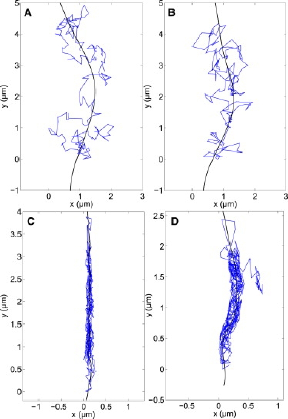
Trajectories A–D plotted with spline curves. (Top left) Trajectory A is a random walk simulated to model experimental trajectory B. (Top right) Trajectory B is an experimental trajectory showing two-dimensional diffusion that is easily analyzed with conventional two-dimensional MSD analysis. (Bottom left) Trajectory C shows linear, confined motion that is more difficult to analyze using conventional two-dimensional MSD. (Bottom right) Trajectory D shows spatial confinement to a curvilinear structure, which is ill suited for conventional two-dimensional MSD analysis, but ideal for the spline-curve analysis techniques discussed in the text. Trajectories B–D were collected from movement of QD probes incubated with PC12 cells (see Methods).

Random walk simulations

Two-dimensional diffusive trajectory A was simulated to model example SPT trajectory B. The trajectory was obtained by vectorially summing N random displacements (Δx,Δy). The values Δx and Δy were random variables drawn from a Gaussian distribution with zero mean and variance σ² = 2D_Bτ, where D_B = 0.22 μm²/s is the two-dimensional diffusion coefficient for trajectory B and τ = 0.06 s is the lag between position measurements in the experimental data. The number of data points of trajectory A was chosen to match that of B (N_A = N_B = 187). MSD plots for trajectories A and B (Fig. 3, top left) show that experimental trajectory B is comparable to a purely diffusive trajectory over the time range of interest, validating the use of a two-dimensional random walk as a model for trajectory B. It is worth noting here that whereas trajectory B may seem to be nonrandom due to its large aspect ratio ɛ = 2.47, comparison to aspect ratios of 5000 random walks with the same number of data points indicates that roughly 17% of random walks would have a larger aspect ratio than trajectory B. (For a detailed discussion of the distribution of asymmetry factors similar to aspect ratio ɛ, see (23).)

Figure 3.

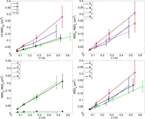
Comparison of conventional two-dimensional MSD analysis and SCDA. (Top left) Conventional two-dimensional MSD plotted for trajectories A–D. Conventional two-dimensional MSD characterizes trajectories C and D with smaller slope (lower D_2D) than that of experimental trajectory B and simulated random walk A, due to the spatial confinement in trajectories C and D. Conventional two-dimensional MSD is plotted here as (1/2) MSD to facilitate comparison with MSD_‖ and MSD_⊥. (Top right) SCDA applied to trajectories A and B shows similar MSD_‖ and MSD_⊥, confirming that the diffusive dynamics of A and B are isotropic and independent of the spline curve. (Bottom left) Trajectories C and D exhibit linear MSD_‖ with nearly identical slopes, showing similar free diffusion along the spline curve. However, MSD_⊥ is severely restricted because the trajectories are spatially confined to be near the spline curve. (Bottom right) Linear MSD_‖ with similar slopes for A–D, showing that all four trajectories have similar diffusive dynamics parallel to their spline curves (D_‖ values are given in Table 1). Error bars in all plots represent the statistical error due to finite sampling (Eq. 3).

A set of 500 two-dimensional random walk trajectories (N = 344, σ² = 2(0.24 μm²/s)τ) was created using the above methods and used to compare conventional MSD and SCDA as described in Results. Additionally, 500 two-dimensional random walk trajectories were mapped onto the surface of a cylinder with radius r = 100 nm and its axis along the x axis. The resulting cylindrical trajectories were projected into the x,y plane to simulate measured confined trajectories of fluorescent particles diffusing on a cylindrical surface contained within the microscope's depth of field.

Measurement of receptor-bound quantum dot trajectories in cells

The NGF-QD probe was prepared using biotin-streptavidin conjugation; details of probe preparation and methods for cell culture and NGF-QD treatment of PC12 cells (ATCC, Manassas, VA) are described in Rajan et al. (38). Sequential fluorescence images of the NGF-QD probes were imaged at a rate of 16.7 frames/s using an inverted microscope in epifluorescence configuration (Axiovert 200m; Zeiss, Oberkochen, Germany) with a 100× 1.4 NA oil immersion objective and a cooled charge-coupled device camera (Axiocam, Zeiss) configured with 2×2 binning. Image files were converted from ZVI format to TIFF stacks using the Bio-Formats Java library (http://www.loci.wisc.edu/ome/formats.html). Particle location and trajectory linking was performed using customized versions of publicly-available MATLAB scripts (http://physics.georgetown.edu/matlab/code.html) that follow the methods described in Crocker and Grier (39). Trajectories B–D plotted in Fig. 1 are example trajectories chosen for varied spatial structure and length (number of data points N_B = 187, N_C = 365, and N_D = 335, and total time T_A = T_B = 11 s, T_C = 22 s, and T_D = 20 s). Uncertainty in particle position measurements, σ_m, was estimated using the correlation between adjacent displacements from Wang et al. (26),

$${\sigma }_{\text{m}}^2=-\langle \Delta x_{\text{i}}\Delta x_{\text{i}+1}\rangle ,$$

and ranged from ±20 nm to ±50 nm for trajectories B–D.

Conventional two-dimensional MSD analysis

Conventional two-dimensional MSD analysis here refers to the calculation of MSD (Eq. 1) and interpretation of the slope of the MSD line as the diffusion coefficient of the particle, D_2D. Each MSD data point was averaged only over adjacent (nonoverlapping) intervals and here we have chosen intervals of Δt = τ, 2τ, 4τ, and 8τ where τ = 0.06 s is the time between frames of the original data. D_2D was calculated from the first data point, i.e., D_2D = MSD(τ)/4τ, and error bars in Fig. 3 and Table 1 are the expected statistical error due to finite sample size (Eq. 3), as discussed in the literature (22,26). For our data, measurement errors σ_m² associated with using the first point of the MSD plot to calculate D are on the same order of magnitude as, but within, the statistical error bars due to finite sampling. Although the correlation 〈Δx_iΔx_i+1〉 can be used to correct MSD for measurement error in unconfined, purely diffusive trajectories (26), both measurement error and actual displacement correlations (e.g., due to confinement) may be combined into our σ_m². We use the first point of the MSD to minimize statistical error, for simplicity, and because correlation error cannot be separated from measurement error in our trajectories. Conventional two-dimensional MSD (Fig. 3, top left) is plotted as (1/2) MSD to facilitate comparison with MSD_|| and MSD_⊥.

Table 1.

Measured values for D_2D, D_‖, and D_⊥ from the example trajectories A–D

	D2D (μm2/s)	D‖ (μm2/s)	D⊥ (μm2/s)
A	0.21 ± 0.02	0.22 ± 0.02	0.20 ± 0.02
B	0.22 ± 0.02	0.21 ± 0.02	0.23 ± 0.02
C	0.091 ± 0.007	0.16 ± 0.01	0.017 ± 0.001
D	0.13 ± 0.01	0.21 ± 0.02	0.053 ± 0.004

Conventional two-dimensional MSD analysis shows different values of D_2D, suggesting differences in the Brownian dynamics of trajectories A and B from C and D. SCDA shows very similar values for D_‖, indicating that these trajectories actually exhibit similar underlying diffusive motion, but differing degrees of confinement lead to varying D_2D values. Errors are statistical uncertainty due to finite sample size.

Spline-curve analysis

We have developed spline-curve analysis methods to produce a curve that characterizes the overall, curvilinear shape of extended trajectories (e.g., trajectories with aspect ratio ɛ ≥ 1.75). We have focused on extended trajectories with curvilinear shapes, and our method is general enough to accommodate trajectories of diffusion in curvilinear structures. In such trajectories, a particle may retrace its position along the structure many times randomly, and so our spline curve is based on the set of particle locations only, not on the time ordering of those locations. We show in Results that the curvilinear shapes of our trajectories can be explained by diffusion in curvilinear confining geometries.

SCDA and SCSA both utilize a spline curve fit to the overall shape of each trajectory. Our spline-fitting methods use two steps: first, choosing points that characterize the overall shape of the curve; and second, generating a spline curve constrained to pass through those points. We developed two methods for choosing points to characterize the overall shape of the curve:

• 1.User-chosen points. Using custom-written presentation software, a user selects typically 5–10 (x, y) points by clicking with a mouse on each plotted trajectory. This process takes a few seconds per trajectory and can be combined with any other trajectory analysis steps that require human intervention.
• 2.Computer-generated points (see also Supporting Material). The (x, y) points were generated in an iterative manner designed to trace out the overall shape of curvilinear trajectories. Each trajectory is divided into n equal segments along e_major, the direction of the trajectory's greatest extent. The value σ_n, the standard deviation about the mean along the direction perpendicular to e_major, is calculated over the trajectory points in each segment. The mean of these n local standard deviations, 〈σ_n〉, provides an estimate of the local width of a curvilinear trajectory that is more accurate than the global standard deviation perpendicular to e_major of the whole trajectory. The global estimate overestimates the local width of curvilinear trajectories.

The width 〈σ_n〉 is used as a characteristic length scale for generating points to characterize the spline curve as follows:

• 1.The first point is the center-of-mass of particle locations within a radius r₁ = 3 〈σ_n〉 of the end of the trajectory along e_major.
• 2.The second point is determined by finding the center-of-mass of particles in the π/2 radian section of an annulus, r₁ < r < 2r₁, that is directed toward the angle with the highest number of particles within π/2 radians.
• 3.This second point is then used as the center of the annulus for choosing the third point, and the process is repeated.

To ensure that each point is ahead of the previous one, and to reduce spurious turns in the spline curve, the angle between each segment and the next point is limited to be <0.2π. If no particle locations are found in the annulus r₁ < r < 2r₁, r₁ is increased to r₁ = 6 〈σ_n〉, and if particles are found within the expanded annulus, the iteration process continues. If no particles are found within r = 12 〈σ_n〉, the iterations stop. Two additional points are then added on each end of the automatically generated points so that the fitted spline curve continues beyond the extent of the trajectory. All results in this article have been automatically analyzed using spline curves derived from computer-generated points with n = 7 and r₁ = 3 〈σ_n〉. These values were chosen based on the four example trajectories in Fig. 1 and were well suited for the random walk simulations and the 159 SPT trajectories analyzed.

Spline-curve fitting

Once the points have been selected either automatically or by hand, a spline curve of 10,000 interpolated points is fit to the points to create a smooth curve that characterizes the overall shape of the trajectory. The spline curve is fit to the selected points using a built-in MATLAB (The MathWorks, Natick, MA) function that generates a piecewise-cubic Hermite polynomial with coefficients chosen so that the curve's value, first derivative, and second derivative are all continuous at each of the selected points. The four trajectories analyzed here (A–D) are shown with spline curves in Fig. 1.

SCDA

Each displacement Δ between successive positions was resolved into components parallel (Δ_‖) and perpendicular (Δ_⊥) to the local tangent to the spline curve (as sketched in Fig. 2, top). This generated a series of parallel displacements and a series of perpendicular displacements. These two series of displacements were then independently analyzed to measure the dependence of MSD_⊥ and MSD_‖ on Δt. MSD_⊥ and MSD_‖ are plotted versus Δt for trajectories A and B (Fig. 3, top) and for trajectories C and D (Fig. 3, bottom). From the first point of MSD_⊥ and MSD_‖ data, we calculated D_⊥, the diffusion coefficient perpendicular to the spline curve, and D_‖, the diffusion coefficient parallel to the spline curve, reported in Table 1. D_‖ and D_⊥ are each treated here as effective one-dimensional diffusion coefficients corresponding to motion along a single coordinate.

Figure 2.

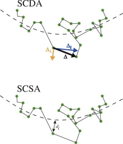
(Top) Spline-curve dynamics analysis (SCDA). A spline curve (dashed line) is fitted through the overall trajectory shape and each displacement Δ is resolved into a component parallel to the spline curve Δ_‖ and a component perpendicular to the spline curve Δ_⊥. The parallel and perpendicular displacements can then be analyzed independently to measure dynamics parallel and perpendicular to the spline curve. (Bottom) Spline-curve spatial analysis (SCSA). The distance d_i from each particle to the spline curve is calculated and histograms of d_i provide a spatial profile of the trajectory.

SCSA

After the spline curve was fit to a trajectory, the shortest distance d_i from each point to the spline curve was measured (as sketched in Fig. 2, bottom). A histogram of d_i was plotted, displaying the spatial distribution of particle positions around the spline curve. Spatial distributions for trajectories A–D are shown in Fig. 5. The stated width of each spatial distribution in Fig. 5 was calculated using the standard deviation about the mean.

Figure 5.

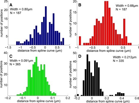
Results of SCSA showing the distribution of distances from the spline curve for trajectories A–D as indicated. Width indicated is the standard deviation about the mean and N is the number of data points. Trajectories A and B show broad spatial distributions (top), whereas C and D show clear confinement near the fitted spline curve (bottom). Additionally, trajectory D exhibits a bimodal distribution, consistent with trajectory positions distributed on a cylindrical surface projected onto the image plane, as described in Results and Fig. 5.

Cylindrical spatial distribution

A simple numerical calculation was performed to model the bimodal spatial distribution of trajectory D. We assume that the actual particle locations are distributed uniformly on a cylindrical shell (radius r = 90 nm, thickness t = 3 nm), excluding the bottom 3 nm, which is presumably in contact with a surface, thus preventing QDs from diffusing there. The shell thickness, t, was chosen here to model the membrane thickness, as it is unclear from our data whether the QD probe is located on the inner or outer surface of or within the membrane. To simulate the experimental uncertainty in QD position measurement, the measured particle locations are distributed with a Gaussian profile in the x direction, with width σ_m = 27 nm. This density of measured particle locations was modeled discretely as a 1000 × 1000 matrix and is plotted in Fig. 6 (top). The spatial distribution along the x axis (Fig. 6, bottom) was created by summing the array values along the z axis.

Figure 6.

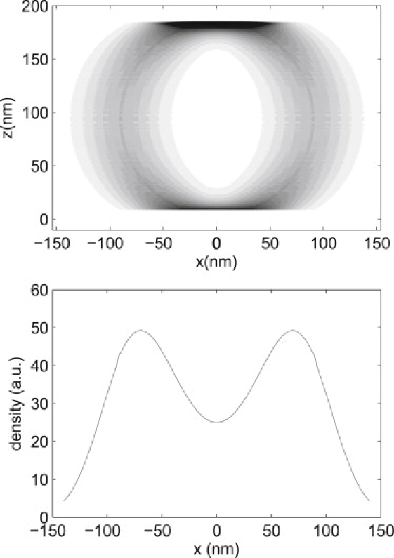
(Top) Simple model of the distribution of measured position locations on a cylindrical shell. The cylinder has radius r = 90 nm and thickness 3 nm, with the bottom 3 nm excluded to model the region in contact with a surface. The density of measured positions is normal-distributed in the x direction corresponding to position measurement error of σ_m ± 27 nm. (Bottom) Projection of this cylindrical distribution onto the x axis, displaying a bimodal distribution similar to that seen in the spatial distribution of trajectory D (Fig. 5, bottom right).

All calculations were performed using MATLAB R2007b on a PC.

Results

In this section, we detail the results of applying SCDA and SCSA to SPT trajectories and simulated random walk trajectories and compare our results to conventional two-dimensional MSD analysis. Both SCDA and SCSA use a spline curve fitted to the overall spatial structure of a trajectory (Fig. 2). SCDA quantifies diffusive motion parallel and perpendicular to the spline curve, characterized by D_‖ and D_⊥, and SCSA extracts spatial features from SPT trajectories by measuring the distribution of distances from measured positions to the spline curve. The spatial features of confined trajectories revealed by SCSA and the diffusive dynamics measured by SCDA can be combined to show that the complex spatial confinements exhibited by example trajectories are consistent with diffusive motion on submicron three-dimensional cellular structures, including diffusion on tunneling nanotubes (40,41). We have applied our methods to a library of 159 experimental SPT trajectories, as well as to a set of 500 two-dimensional random walk simulations of normal diffusion and a set of 500 cylindrically confined random walk simulations. We demonstrate our methods in detail on four example trajectories, including one random walk simulation (A) and three SPT trajectories of QD probes (B–D) (Fig. 1) collected as described in Methods.

Dynamics: SCDA and conventional two-dimensional MSD analysis

SCDA resolves the dynamics of a trajectory into displacements parallel and perpendicular to the fitted spline curve (as sketched in Fig. 2, top). The parallel and perpendicular motion can then be independently analyzed to yield MSD_‖ and MSD_⊥, and associated diffusion coefficients D_‖ and D_⊥, as described in Methods. Conventional two-dimensional MSD analysis of example trajectories A–D yields MSD plots (Fig. 3, top left) and D_2D values (Table 1), which show lower values of D_2D for trajectories C and D than trajectories A and B. According to the conventional interpretation of these data, these lower values of D_2D reflect differences in parameters governing underlying microscopic Brownian dynamics, such as temperature, particle size, or viscosity of the medium.

Applying SCDA to trajectories A–D yields MSD_‖ and MSD_⊥ (Fig. 3) and the associated values for D_⊥ and D_‖ (Table 1). Values of MSD_⊥ are almost unchanged over time for C and D (Fig. 3, bottom left), and so very small diffusion coefficients characterize motion perpendicular to the spline curve (D_⊥ = 0.017 ± 0.001 and D_⊥ = 0.053 ± 0.004 μm²/s for C and D, respectively). These small D_⊥ values are expected because particle displacements perpendicular to the spline curve are restricted to be less than the size of the confining structure for trajectories with clear curvilinear confinement. Notably, MSD_‖ plots are linear for all three SPT trajectories, indicating diffusive motion parallel to the spline curve (Fig. 3, bottom right). This analysis shows that the underlying microscopic motion in trajectories C and D is Brownian, but is also constrained by the local confining geometry. Despite the fact that the example trajectories are characterized by a wide range of D_2D values, qualitatively different shapes and varying spatial confinement, they all have similar D_‖ values.

To validate the SCDA results from trajectories A–D, we applied SCDA to 500 two-dimensional random walk trajectories simulating free diffusion and 500 random walk trajectories confined to the surface of a 100-nm cylinder. For purely diffusive trajectories, SCDA recapitulates the results of conventional two-dimensional MSD analysis. Fig. 4 (left) shows that distributions of D_‖, D_⊥, and D_2D values have nearly identical means. However, SCDA and conventional two-dimensional MSD analysis yield clearly different results when applied to simulated random walks confined to a cylindrical surface. In Fig. 4 (center), distributions of D_‖, D_⊥, and D_2D show that D_| reproduces the true, microscopic two-dimensional diffusion coefficient (random walk D = 0.24 μm²/s). D_2D, on the other hand, systematically underestimates D by ∼50% because of the lateral confinement which reduces the measured D_⊥ values. This underestimation of D is also shown when we applied SCDA to a library of 159 curvilinear SPT trajectories of QD probes. The distributions of diffusion coefficients in Fig. 4 (right) show that D_2D is strongly influenced by the restricted diffusion in the perpendicular direction, whereas D_‖ shows a wide range of values that are larger than the diffusion coefficient D_2D reported by conventional two-dimensional MSD analysis.

Figure 4.

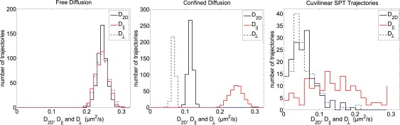
Distributions of diffusion coefficients D_2D, D_‖, and D_⊥ for free diffusion, confined diffusion, and curvilinear SPT trajectories. (Left) D_2D, D_‖, and D_⊥ from 500 two-dimensional random walk trajectories simulating purely diffusive motion. D_‖ and D_⊥ reproduce the diffusion coefficient D_2D obtained using conventional two-dimensional MSD analysis. (Center) D_2D, D_‖, and D_⊥ from the two-dimensional projections of 500 two-dimensional random walk trajectories confined to a 100-nm radius cylinder. D_2D systematically underestimates the true diffusion coefficient, D = 0.24 μm²/s. D_‖ provides a more accurate measure of D because the unconfined motion along the spline curve is separated from the confined motion perpendicular to the spline curve. (Right) D_2D, D_‖, and D_⊥ from 159 curvilinear SPT trajectories. The range of D_‖ values includes a wide range of larger values than those reported by D_2D, illustrating that conventional two-dimensional MSD also underestimates diffusion in experimental trajectories.

Close examination of three example trajectories (B–D) from the library of 159 SPT trajectories reveals similar D_‖ values among trajectories with disparate appearances. These D_‖ values indicate that trajectories B–D measure the motion of QD probes experiencing similar local, microscopic dynamics despite different confinement geometries. The differences between D_2D and D_‖ values in Table 1 and the distributions of diffusion coefficients in Fig. 4 illustrate a limitation of conventional two-dimensional MSD analysis: Eq. 1 treats each displacement in the confined trajectories equally, and does not distinguish between the confined diffusion perpendicular to the spline curve and the unconfined motion parallel to it. As a result, a combination of confined and unconfined motion leads to lower D_2D for confined trajectories such as C and D, and the majority of the 159 curvilinear SPT trajectories were analyzed in Fig. 4 (right). In contrast to conventional two-dimensional MSD analysis, SCDA separates parallel and perpendicular dynamics and recovers the unconfined, microscopic Brownian motion parallel to the spline curve, as characterized by D_‖. The SCDA-extracted values of D_‖ provide a more accurate measurement of microscopic diffusion in confined trajectories. These confined dynamics commonly arise as the result of motion confined by subcellular structures or movement on complex surfaces of plasma membranes.

Mapping subdiffraction spatial structure from trajectories using SCSA

SCSA quantifies the spatial confinement of SPT trajectories that can sometimes be visible by eye in x-y plots with subdiffraction resolution (e.g., trajectories C and D in Fig. 1). Subdiffraction-limit spatial resolution is accessible here because each particle location is measured from a separate image with estimated position error σ_m = ±20–50 nm. The distance d_i is calculated from each point to the spline curve, independent of its order in the trajectory and its location along the curve (see sketch in Fig. 2, bottom). This spatial information is also static and independent of the dynamic information (D_⊥, D_‖) obtained using SCDA. Fig. 5 shows the distribution of particle positions relative to the spline curve, revealing the transverse spatial profile of the trajectory and quantifying the range of visible spatial confinement seen in x-y plots of the trajectories in Fig. 1. The spatial distributions for trajectories A and B are broad and show no spatial confinement (Fig. 5, top), whereas trajectories C and D show clear confinement to regions a few hundred nanometers from their respective spline curves (Fig. 5, bottom). The bimodal distribution for trajectory D is especially striking (Fig. 5, bottom right), clearly quantifying spatial structure below the diffraction limit (≈230 nm).

Further capabilities of SCDA and SCSA

By combining information of diffusive dynamics and subdiffraction spatial structure, results of SCDA and SCSA can assist in interpreting the spatial geometry of cellular three-dimensional structures from two-dimensional trajectories. One important aspect of SPT trajectories is that they are two-dimensional projections of three-dimensional movement within the microscope's depth of field. Our example trajectories A–D and the results of SCDA and SCSA highlight the importance of considering this three-dimensional motion when interpreting two-dimensional SPT trajectory data.

SCSA and SCDA can identify isotropic, unconfined diffusive movement characteristic of motion on a flat surface. In our data, example trajectories A and B show linear MSD_‖ and MSD_⊥ with similar slopes (Fig. 3, top right), implying similar Brownian motion parallel and perpendicular to the spline curves over the measured range of Δt. SCSA corroborates this result: there is no clear spatial confinement in trajectories A and B, as seen by the broad distributions of distances from the spline curve (Fig. 5, top). The isotropy of Brownian motion in trajectory B, as well as its spatial and dynamic similarities with the two-dimensional random walk trajectory A, lead us to infer that trajectory B represents the two-dimensional Brownian motion within the depth of field of the microscope. We conclude that trajectory B measures the motion of a QD probe on a flat portion of the cell membrane. The values of D_‖ are consistent with published diffusion coefficients for NGF receptor proteins in the plasma membrane of PC12 cells (42).

The combined results of SCSA and SCDA can lead to a consistent picture of local three-dimensional spatial structure and microscopic dynamics from individual SPT trajectories. For example, SCSA yields the bimodal spatial profile for trajectory D (Fig. 5, bottom right), which indicates that particle positions are preferentially distributed along both sides of the fitted spline curve, with two peaks of the distribution separated by d ≈ 160 nm. This bimodal distribution is consistent with the two-dimensional projection of particle locations distributed over a cylindrical shell as shown in Fig. 6. Such a cylindrical structure is smaller in diameter than the microscope's depth of field, so all z positions on the cylinder can be captured in focus. The high spatial resolution of SCSA data is necessary for this interpretation: if a cylindrical shell of diameter d ≈ 120 nm were uniformly labeled with a fluorescent dye, optical diffraction would blur the bimodal distribution, making the two peaks irresolvable. Dynamic information from SCDA of trajectory D reveals the dynamics of the QD probe on this cylindrical structure. Here, MSD_‖ is linear and its measured D_‖ is comparable to that of the other example trajectories (Fig. 3, bottom right), indicating Brownian motion along the spline curve. Furthermore, the local, microscopic diffusion coefficient along the structure (D_‖) is similar to that of free two-dimensional diffusion in trajectory B and within the range of published values of D_2D for NGF receptors in the plasma membrane. Taken together, SCSA and SCDA provide evidence that trajectory D is the two-dimensional projection of diffusion on the surface of a cylindrical plasma membrane structure with radius r ≈ 80 nm. These cylindrical spatial structures (as represented by bimodal spatial distributions) were seen in 10 out of 159 experimental trajectories, with radii 50 > r > 100 nm. The size of these spatial structures and the D_‖ values that we measure are consistent with the movement of particles along tunneling nanotubes observed in PC12 and other cell cultures (32,40,41).

Discussion

Extending MSD analysis to include curvilinear trajectories

Conventional two-dimensional MSD analysis is often used to measure D_2D from an ensemble of particle trajectories. However, not all trajectories are suitable for conventional two-dimensional MSD analysis. For example, particles in trajectories C and D are confined to curvilinear structures and therefore violate the underlying assumptions of conventional two-dimensional MSD analysis. Inclusion of these trajectories in two-dimensional MSD analysis gives spuriously low values of D_2D, as discussed in Results. Spline-curve methods extend the capabilities of conventional MSD analysis to include trajectories confined to curvilinear structures: trajectories with curvilinear spatial structure can be fitted to a spline curve and the motion parallel and perpendicular to the spline curve can each be analyzed independently. D_‖ provides a more accurate measure of microscopic diffusive dynamics than D_2D, because the spline curve takes into account the local geometry of the trajectory.

Implementation, spline-curve variation, and limitations

The automated implementation of our method involves using computer-chosen points to generate each spline curve (see Methods and Supporting Material). The automated method generates spline curves based only on the shape of the trajectory, and does not rely on an external input for determining r₁, the only length-scale used in determining the spline curve. This scale-independence of SCSA and SCDA allows the algorithms to be applied to trajectories of any size. As a result, the methods do not impose any a priori limitations on the absolute size of features characterized by the spline curve. Our method of calculating r₁ from each trajectory individually works well for our experimental SPT data and random walk simulations, and may be adjusted to accommodate other types of trajectories as needed. Similarly, the computer-chosen points are best suited to extended, curvilinear trajectories, because they are restricted to have a maximum angle between the n sequential points of θ_max = 0.2π, yielding a minimum radius of curvature r_c ≤ r₁/θ_max.

This automated implementation requires no user supervision once θ_max = 0.2π and the method for calculating r₁ have been selected, so large amounts of SPT trajectory data can be quickly analyzed. However, the streamlining associated with automating this process (as opposed to a user choosing points by eye for each trajectory) comes at the cost of flexibility. Random variations in the density of particle locations along an otherwise uniform curvilinear trajectory can lead to deviations in the spline curve that a human user would intuitively avoid in selecting points by eye.

We have developed our method to extract spatial and dynamic information from confined, curvilinear trajectories, and as such, we are limited in the types of structures that can be characterized with our method. For example, characterizing motion confined to branched or circular structures is outside the range of suitable trajectories for our method; such trajectories result in the spline curve missing the overall shape of the trajectory and subsequently inaccurate SCSA and SCDA results.

A key benefit of spline-curve analysis is its flexibility to quantify anisotropic dynamics via D_‖ and D_⊥ for a wide range of trajectory shapes. The anisotropic dynamics of linear trajectories such as C could be partially accessible through independent analysis of x and y displacements in a suitably rotated coordinate system (e.g., (31,37)). However, the complex spatial structures of trajectories such as D prevent its dynamics from being resolvable by a global coordinate rotation. Our spline-curve methods allow the resolution of anisotropic dynamics from these trajectories that exhibit more complex, curvilinear spatial confinement. We note that a curvilinear coordinate system similar to our spline-curve methods has been recently used to improve step-finding analysis of myosin V motion (21), demonstrating the broad utility of curvilinear coordinate systems for analysis of confined and anisotropic motion inside cells.

The interpretation of three-dimensional structures from two-dimensional trajectories is difficult, because a two-dimensional projection does not unambiguously determine the original three-dimensional structure. However, qualitative features of SCDA spatial distributions can identify three-dimensional geometries that are consistent with measured trajectory data. For example, the bimodal spatial distribution of trajectory D is consistent with diffusion on the surface of a cylinder, but not with diffusion inside a cylinder. For particle positions from two-dimensional trajectories to faithfully represent the projection of three-dimensional structures, the measured particle positions must be evenly distributed over the three-dimensional structure. Even if this condition is met, different possible three-dimensional geometries could be projected to form a given two-dimensional trajectory. This is the case of example trajectory C, which could be the two-dimensional projection of diffusive motion on a linear structure, or on a planar structure viewed edge-on. In the future, three-dimensional tracking and three-dimensional superresolution imaging methods could be used to corroborate our interpretation of the results from SCDA and SCSA.

Our SCDA and SCSA methods calculate D_‖, D_⊥, and the spatial profile over each entire trajectory, so any variations in the dynamics or spatial confinement within a trajectory are folded into average quantities. For this reason, it is most straightforward to interpret the results of SCDA and SCSA when the dynamics are uniformly diffusive on a curvilinear structure with constant cross section. To quantify variation within a single trajectory, SPT trajectories with more data points are needed. For our SPT trajectories (number of datapoints N ∼10²), statistical error in D measurements is roughly 10% (see Table 1), and subdividing the trajectory would increase this statistical error in D (see Eq. 3). However, for trajectories with N ∼10³ or greater, SCDA and SCSA could be extended to measure varied dynamics or spatial confinement in subsegments of trajectories.

Future applications

Spline-curve analysis opens the door to several new avenues of extracting meaningful information from particle trajectories in cells. For example, quantifiable trajectory features could be correlated with biomarkers of interest by associating characteristics of the local dynamics and confining geometry, such as the width of the spatial distribution and D_‖ and D_⊥, with fluorescently-labeled antibodies for specific proteins. Such a tool combined with a validated probe has the potential to identify the intracellular location of biomolecules with high spatial resolution directly from SPT trajectories alone. Another application is to differentiate between Brownian motion and active transport in confined SPT trajectories, which would be possible with improved temporal resolution and more detailed analysis of dynamics parallel and perpendicular to the spline curves. For example, the motion of endosomes undergoing active transport could be confined to a particular linear or tubular structure, but the active transport along such a structure should be characterized by non-Gaussian displacement distributions and nonlinear MSD, not the Brownian motion seen in our example trajectories. With improved resolution, our spline-curve methods could be used to separate the effects of particle confinement from the effects of active transport on measured two-dimensional trajectories.

Supporting Material

Four figures illustrating automated spline-curve analysis are available at http://www.biophysj.org/biophysj/supplemental/S0006-3495(09)06152-9.

References

- 1.Saxton M.J., Jacobson K. Single-particle tracking: applications to membrane dynamics. Annu. Rev. Biophys. Biomol. Struct. 1997;26:373–399. doi: 10.1146/annurev.biophys.26.1.373. [DOI] [PubMed] [Google Scholar]
- 2.Inoue A., Okabe S. The dynamic organization of postsynaptic proteins: translocating molecules regulate synaptic function. Curr. Opin. Neurobiol. 2003;13:332–340. doi: 10.1016/s0959-4388(03)00077-1. [DOI] [PubMed] [Google Scholar]
- 3.Chang Y.-P., Pinaud F., Weiss S. Tracking bio-molecules in live cells using quantum dots. J. Biophotonics. 2008;1:287–298. doi: 10.1002/jbio.200810029. [DOI] [PMC free article] [PubMed] [Google Scholar]
- 4.Wieser S., Schütz G.J. Tracking single molecules in the live cell plasma membrane—do's and don't's. Methods. 2008;46:131–140. doi: 10.1016/j.ymeth.2008.06.010. [DOI] [PubMed] [Google Scholar]
- 5.Levi V., Gratton E. Exploring dynamics in living cells by tracking single particles. Cell Biochem. Biophys. 2007;48:1–15. doi: 10.1007/s12013-007-0010-0. [DOI] [PubMed] [Google Scholar]
- 6.Goulian M., Simon S.M. Tracking single proteins within cells. Biophys. J. 2000;79:2188–2198. doi: 10.1016/S0006-3495(00)76467-8. [DOI] [PMC free article] [PubMed] [Google Scholar]
- 7.Jin S., Verkman A.S. Single particle tracking of complex diffusion in membranes: simulation and detection of barrier, raft, and interaction phenomena. J. Phys. Chem. B. 2007;111:3625–3632. doi: 10.1021/jp067187m. [DOI] [PubMed] [Google Scholar]
- 8.Brandenburg B., Zhuang X. Virus trafficking—learning from single-virus tracking. Nat. Rev. Microbiol. 2007;5:197–208. doi: 10.1038/nrmicro1615. [DOI] [PMC free article] [PubMed] [Google Scholar]
- 9.Haggie P.M., Kim J.K., Verkman A.S. Tracking of quantum dot-labeled CFTR shows near immobilization by C-terminal PDZ interactions. Mol. Biol. Cell. 2006;17:4937–4945. doi: 10.1091/mbc.E06-08-0670. [DOI] [PMC free article] [PubMed] [Google Scholar]
- 10.Suzuki K., Ritchie K., Kusumi A. Rapid hop diffusion of a G-protein-coupled receptor in the plasma membrane as revealed by single-molecule techniques. Biophys. J. 2005;88:3659–3680. doi: 10.1529/biophysj.104.048538. [DOI] [PMC free article] [PubMed] [Google Scholar]
- 11.Kusumi A., Nakada C., Fujiwara T. Paradigm shift of the plasma membrane concept from the two-dimensional continuum fluid to the partitioned fluid: high-speed single-molecule tracking of membrane molecules. Annu. Rev. Biophys. Biomol. Struct. 2005;34:351–378. doi: 10.1146/annurev.biophys.34.040204.144637. [DOI] [PubMed] [Google Scholar]
- 12.Kusumi A., Sako Y. Cell surface organization by the membrane skeleton. Curr. Opin. Cell Biol. 1996;8:566–574. doi: 10.1016/s0955-0674(96)80036-6. [DOI] [PubMed] [Google Scholar]
- 13.Lidke D.S., Lidke K.A., Arndt-Jovin D.J. Reaching out for signals: filopodia sense EGF and respond by directed retrograde transport of activated receptors. J. Cell Biol. 2005;170:619–626. doi: 10.1083/jcb.200503140. [DOI] [PMC free article] [PubMed] [Google Scholar]
- 14.Andrews N.L., Lidke K.A., Lidke D.S. Actin restricts FcɛRI diffusion and facilitates antigen-induced receptor immobilization. Nat. Cell Biol. 2008;10:955–963. doi: 10.1038/ncb1755. [DOI] [PMC free article] [PubMed] [Google Scholar]
- 15.Dahan M., Lévi S., Triller A. Diffusion dynamics of glycine receptors revealed by single-quantum dot tracking. Science. 2003;302:442–445. doi: 10.1126/science.1088525. [DOI] [PubMed] [Google Scholar]
- 16.Jaskolski F., Henley J.M. Synaptic receptor trafficking: the lateral point of view. Neuroscience. 2009;158:19–24. doi: 10.1016/j.neuroscience.2008.01.075. [DOI] [PMC free article] [PubMed] [Google Scholar]
- 17.Triller A., Choquet D. New concepts in synaptic biology derived from single-molecule imaging. Neuron. 2008;59:359–374. doi: 10.1016/j.neuron.2008.06.022. [DOI] [PubMed] [Google Scholar]
- 18.Watanabe T.M., Higuchi H. Stepwise movements in vesicle transport of HER2 by motor proteins in living cells. Biophys. J. 2007;92:4109–4120. doi: 10.1529/biophysj.106.094649. [DOI] [PMC free article] [PubMed] [Google Scholar]
- 19.Kural C., Serpinskaya A.S., Selvin P.R. Tracking melanosomes inside a cell to study molecular motors and their interaction. Proc. Natl. Acad. Sci. USA. 2007;104:5378–5382. doi: 10.1073/pnas.0700145104. [DOI] [PMC free article] [PubMed] [Google Scholar]
- 20.Courty S., Luccardini C., Dahan M. Tracking individual kinesin motors in living cells using single quantum-dot imaging. Nano Lett. 2006;6:1491–1495. doi: 10.1021/nl060921t. [DOI] [PubMed] [Google Scholar]
- 21.Pierobon P., Achouri S., Cappello G. Velocity, processivity, and individual steps of single myosin V molecules in live cells. Biophys. J. 2009;96:4268–4275. doi: 10.1016/j.bpj.2009.02.045. [DOI] [PMC free article] [PubMed] [Google Scholar]
- 22.Qian H., Sheetz M.P., Elson E.L. Single particle tracking. Analysis of diffusion and flow in two-dimensional systems. Biophys. J. 1991;60:910–921. doi: 10.1016/S0006-3495(91)82125-7. [DOI] [PMC free article] [PubMed] [Google Scholar]
- 23.Saxton M.J. Lateral diffusion in an archipelago. Single-particle diffusion. Biophys. J. 1993;64:1766–1780. doi: 10.1016/S0006-3495(93)81548-0. [DOI] [PMC free article] [PubMed] [Google Scholar]
- 24.Saxton M.J. Single-particle tracking: models of directed transport. Biophys. J. 1994;67:2110–2119. doi: 10.1016/S0006-3495(94)80694-0. [DOI] [PMC free article] [PubMed] [Google Scholar]
- 25.Saxton M.J. Single-particle tracking: the distribution of diffusion coefficients. Biophys. J. 1997;72:1744–1753. doi: 10.1016/S0006-3495(97)78820-9. [DOI] [PMC free article] [PubMed] [Google Scholar]
- 26.Wang Y.M., Flyvbjerg H., Austin R.H. Lecture Notes in Physics: Controlled Nanoscale Motion. Vol. 711/2007. Springer; Berlin, Heidelberg, Germany: 2007. [Google Scholar]
- 27.Shtengel G., Galbraith J.A., Hess H.F. Interferometric fluorescent super-resolution microscopy resolves 3D cellular ultrastructure. Proc. Natl. Acad. Sci. USA. 2009;106:3125–3130. doi: 10.1073/pnas.0813131106. [DOI] [PMC free article] [PubMed] [Google Scholar]
- 28.Huang B., Wang W., Zhuang X. Three-dimensional super-resolution imaging by stochastic optical reconstruction microscopy. Science. 2008;319:810–813. doi: 10.1126/science.1153529. [DOI] [PMC free article] [PubMed] [Google Scholar]
- 29.Ram S., Prabhat P., Ober R.J. High accuracy 3D quantum dot tracking with multifocal plane microscopy for the study of fast intracellular dynamics in live cells. Biophys. J. 2008;95:6025–6043. doi: 10.1529/biophysj.108.140392. [DOI] [PMC free article] [PubMed] [Google Scholar]
- 30.Hall D. Analysis and interpretation of two-dimensional single-particle tracking microscopy measurements: effect of local surface roughness. Anal. Biochem. 2008;377:24–32. doi: 10.1016/j.ab.2008.02.019. [DOI] [PubMed] [Google Scholar]
- 31.Wieser S., Schutz G.J., Stockinger H. Single molecule diffusion analysis on cellular nanotubules: implications on plasma membrane structure below the diffraction limit. Appl. Phys. Lett. 2007;91:233901. http://link.aip.org/link/?APL/91/233901/1 [Google Scholar]
- 32.Lade S.J. Geometric and projection effects in Kramers-Moyal analysis. Phys. Rev. E Stat. Nonlin. Soft Matter Phys. 2009;80:031137. doi: 10.1103/PhysRevE.80.031137. [DOI] [PubMed] [Google Scholar]
- 33.Ribrault C., Triller A., Sekimoto K. Diffusion trajectory of an asymmetric object: information overlooked by the mean square displacement. Phys. Rev. E Stat. Nonlin. Soft Matter Phys. 2007;75:021112. doi: 10.1103/PhysRevE.75.021112. http://link.aps.org/abstract/PRE/v75/e021112 [DOI] [PubMed] [Google Scholar]
- 34.Gov N.S. Diffusion in curved fluid membranes. Phys. Rev. E Stat. Nonlin. Soft Matter Phys. 2006;73:041918. doi: 10.1103/PhysRevE.73.041918. [DOI] [PubMed] [Google Scholar]
- 35.Auth T., Gov N.S. Diffusion in a fluid membrane with a flexible cortical cytoskeleton. Biophys. J. 2009;96:818–830. doi: 10.1016/j.bpj.2008.10.038. [DOI] [PMC free article] [PubMed] [Google Scholar]
- 36.Sanabria H., Kubota Y., Waxham M.N. Multiple diffusion mechanisms due to nanostructuring in crowded environments. Biophys. J. 2007;92:313–322. doi: 10.1529/biophysj.106.090498. [DOI] [PMC free article] [PubMed] [Google Scholar]
- 37.Kusumi A., Sako Y., Yamamoto M. Confined lateral diffusion of membrane receptors as studied by single particle tracking (nanovid microscopy). Effects of calcium-induced differentiation in cultured epithelial cells. Biophys. J. 1993;65:2021–2040. doi: 10.1016/S0006-3495(93)81253-0. [DOI] [PMC free article] [PubMed] [Google Scholar]
- 38.Rajan S.S., Liu H.Y., Vu T.Q. Ligand-bound quantum dot probes for studying the molecular scale dynamics of receptor endocytic trafficking in live cells. ACS Nano. 2008;2:1153–1166. doi: 10.1021/nn700399e. [DOI] [PubMed] [Google Scholar]
- 39.Crocker J.C., Grier D.G. Methods of digital video microscopy for colloidal studies. J. Colloid Interface Sci. 1996 http://physics.nyu.edu/grierlab/methods/methods.html [Google Scholar]
- 40.Rustom A., Saffrich R., Gerdes H.H. Nanotubular highways for intercellular organelle transport. Science. 2004;303:1007–1010. doi: 10.1126/science.1093133. [DOI] [PubMed] [Google Scholar]
- 41.Gerdes H.-H., Carvalho R.N. Intercellular transfer mediated by tunneling nanotubes. Curr. Opin. Cell Biol. 2008;20:470–475. doi: 10.1016/j.ceb.2008.03.005. [DOI] [PubMed] [Google Scholar]
- 42.Wolf D.E., McKinnon-Thompson C., Ross A.H. Mobility of TrkA is regulated by phosphorylation and interactions with the low-affinity NGF receptor. Biochemistry. 1998;37:3178–3186. doi: 10.1021/bi9719253. http://dx.doi.org/10.1021/bi9719253 [DOI] [PubMed] [Google Scholar]
Associated Data
This section collects any data citations, data availability statements, or supplementary materials included in this article.