Role of ATP-Hydrolysis in the Dynamics of a Single Actin Filament

Abstract

We study the stochastic dynamics of growth and shrinkage of single actin filaments taking into account insertion, removal, and ATP hydrolysis of subunits either according to the vectorial mechanism or to the random mechanism. In a previous work, we developed a model for a single actin or microtubule filament where hydrolysis occurred according to the vectorial mechanism: the filament could grow only from one end, and was in contact with a reservoir of monomers. Here we extend this approach in two ways—by including the dynamics of both ends and by comparing two possible mechanisms of ATP hydrolysis. Our emphasis is mainly on two possible limiting models for the mechanism of hydrolysis within a single filament, namely the vectorial or the random model. We propose a set of experiments to test the nature of the precise mechanism of hydrolysis within actin filaments.

Introduction

Actin monomers polymerize to form long helical filaments, by addition of monomers at the ends of the filament. The two ends are structurally different. The addition and removal of subunits at one end, the barbed end, are substantially faster than at the other end, the pointed end. In an equilibrium polymer, the critical concentration at which the on- and off-rates are balanced must be the same at both ends for thermodynamic reasons (1). However, actin is not an equilibrium polymer, it is an ATPase, and ATP is rapidly hydrolyzed after polymerization. Due to this constant energy consumption, the actin polymer exhibits many interesting nonequilibrium features; most notably, it is able to maintain different critical concentrations at the two ends (2). This allows the existence of a special steady state called treadmilling, characterized by a flux of subunits going through the filament, which has been observed with actin as well as with microtubules filaments (3).

The precise molecular mechanism of hydrolysis in actin has been controversial for many years. For each of the two steps involved in the hydrolysis (the ATP cleavage and the Pi release), the possibility of the reaction occurring either at the interface between neighboring units carrying different nucleotides or at random location within the filament can be invoked. The vectorial model corresponds to a limit of infinite cooperativity in which the hydrolysis of a given monomer depends entirely on the state of its neighbors, and the random model is a model of zero cooperativity in which the hydrolysis of a given monomer is independent of the state of its neighbors. In between these two limits, models with a finite cooperativity have been considered (4,5). For instance for microtubules, a direct evidence for a cooperative mechanism was brought recently by Dimitrov et al. (6), who observed GTP-tubulin remnants using a specific antibody.

Several groups have emphasized the process of random cleavage followed by random Pi release (7,8). By studying the polymerization of actin in the presence of phosphate, Fujiwara et al. (2) argued that the crucial step of release of the phosphate is not a simple vectorial process but is probably cooperative. Because this release of phosphate is slow, the delay between the completion of hydrolysis and the polymerization can lead to overshoots which indeed have been observed in fluorescence intensity measurements of pyrene-labeled actin during rapid polymerization as discussed in Brooks and Carlsson (9). At the single filament level, the dynamics of depolymerization is also very interesting. The study of this dynamics provides insights into the underlying mechanism of hydrolysis in actin as discussed recently in the literature (5,10).

Although decades of work in the biochemistry of actin have provided many details on the kinetics of self-assembly of actin in the absence and in the presence of actin binding proteins, it is difficult to capture the complexity of this process without a mathematical model to organize all this information. To this end, we have studied a nonequilibrium model for a single actin or microtubule filament (11) based on the work of Stukalin et al. (12). In this model, the hydrolysis of subunits inside the filament is a vectorial process, the filament is in contact with a reservoir of monomers, and growth occurs only from one end. We have analyzed the phase diagram of that model with a special emphasis on the bounded growth phase, and we have discussed some features of the dynamic instability. Our approach differs from previous work on the dynamic instability of microtubules in the following way: the model is formulated in terms of rates associated with monomer addition/removal and hydrolysis rather than in terms of phenomenological parameters such as the switching rates between states of growth and collapse, as done in the literature (13,14). This should be a definite advantage when bridging the gap between the theoretical model and experiments.

The work of Flyvbjerg et al. (14) has inspired a number of other theoretical models, based on a microscopic treatment of growth, decay, catastrophe, and rescue of the filament: see, in particular, Zong et al. (15), Antal et al. (16,17), and Sumedha et al. (18), which analyze several aspects of the dynamic instability of microtubules using analytical and numerical methods.

In this article, we present a model for a single actin filament which accounts for the insertion, removal, and ATP hydrolysis of subunits at both ends. It extends our previous work (11) in several ways: first by including the dynamics of both ends and secondly by carrying out simulations for both mechanisms of hydrolysis—vectorial and random. In the next section, we present the first extension due to the inclusion of both ends, and following that, we study the two versions of the model for the hydrolysis within the filament. In the final section, we examine transient properties of a single filament using numerical simulations and we show that for these transient properties, the vectorial and random models lead to distinct behaviors. This suggests experiments that would allow us to discriminate between the two models.

Vectorial Model of Hydrolysis with Activity at Both Ends

ATP hydrolysis is a two-step process: the first step is the ATP cleavage which produces ADP-Pi, and is rapid. The second step is the release of the phosphate (Pi), which leads to ADP-actin, and is, by comparison, much slower (19). ADP-Pi-actin and ATP-actin have similar critical concentrations but they are kinetically different species, since they have different on- and off-rates as shown in Fujiwara et al. (2). Nevertheless, from a kinetic point of view, the slow step of release of the phosphate is the rate-limiting essential step. This suggests that many kinetic features of actin polymerization can be explained by a simplified model of hydrolysis, which takes into account only the second step of hydrolysis and treats actin subunits bound to ATP and actin subunits bound to ADP-Pi as a single species. This is the assumption of Stukalin and Kolomeisky (12), which we have used in our previously published study (11) as well as in this work. In other words, what is meant by hydrolysis in all these references is the step of Pi release. In this section, we assume that this release of Pi is a vectorial process described as a single reaction with rate R.

Let us recall the main features of the phase diagram of our previous model which assumes that only one end is growing. The model has three different phases: two phases of unbounded growth and one phase of bounded growth. In one phase of unbounded growth (phase III), both the cap and the bulk of the filament are unbounded. In this rapidly growing phase, the filament is essentially made of unhydrolyzed ATP-actin monomers. In the intermediate phase of unbounded growth (phase II), the cap length remains constant as a function of time whereas the length of the filament grows linearly with time. Finally, in the phase of bounded growth (phase I), both cap length and filament length remain constant on average. This phase is characterized by a finite average length 〈l〉 and by a specific length distribution of the filament which were calculated in Ranjith et al. (11). The phase of unbounded growth is frequently observed with actin, whereas the intermediate phase only exists as a steady state in a small interval of concentration of actin monomers near the critical concentration. The intermediate phase can, however, be observed outside this interval in a transient way, by forcing filaments to depolymerize through a dilution of the external medium. The phase of bounded growth of a single filament growing from one end only, has not been observed experimentally so far with actin, but it has been observed and is well known in microtubules (13,14).

We now extend the single-end model by including dynamics at both the ends. We keep, as before, the assumption of vectorial hydrolysis, which means that there is a single interface between the ATP subunit and ADP subunits, and the assumption of a reservoir of free ATP subunits in contact with the filament. The addition of ATP subunits occurs with rate U at the barbed end, and the removal of ATP subunits occurs with rate W_T⁺ at the barbed end and with a rate W_T^– at the pointed end. The removal of ADP subunits occurs at the barbed end only if the cap is zero, with rate W_D⁺. At the pointed end, ADP subunits are removed with a rate W_D^–. Note that we neglect the possibility of addition of ATP subunits at the pointed end; this assumption is not essential, but it simplifies the analysis.

In Figs. 1 and 2, all the moves discussed above have been represented. Furthermore, we have assumed that all the rates are independent of the concentration of free ATP subunits C except for the on-rate which is U = k₀C. All the rates of this model have been determined precisely experimentally except for R. The values of these rates are given in Table 1.

Figure 1.

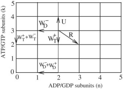
Schematic diagram representing the addition of subunits with rate U, removal with rates W_T⁺, W_T^–, and W_D⁺, and hydrolysis with rate R, which can only occur at the interface between T and D monomers in the vectorial model. Note that two new rates W_T^– and W_D^– have been added as compared to Ranjith et al. (11).

Figure 2.

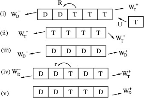
Representation of the various possible moves for actin dynamics. Cases i–iii depict different cases for vectorial hydrolysis. Cases iv and v depict cases for random hydrolysis.

Table 1.

Various rates used in the model and corresponding references

Parameter	Symbol	Value	Ref.
On-rate of T subunits at the barbed end	k0 (μM−1 s−1)	11.6	(1,12)
Off-rate of T subunits at the barbed end	WT+(s−1)	1.4	(1,12)
Off-rate of T subunits at the pointed end	WT–(s−1)	0.8	(1,12)
Off-rate of D subunits at the barbed end	WD+(s−1)	7.2	(1,12)
Off-rate of D subunits at the pointed end	WD–(s−1)	0.27	(1,12)
Hydrolysis rate (vectorial model)	R (s−1)	0.1–0.3	(12)
Hydrolysis rate (random model)	r (s−1)	0.003	(7,9,12)

The condition is that of a low ionic strength buffer.

The state of the filament can be represented in terms of n, the number of ADP subunits, and k, the number of ATP subunits. The dynamics of the filament can be mapped onto that of a random walker in the upper-quarter plane (n, k) with the specific moves as shown in Fig. 1. We find the following steady-state phases (see the Appendix for details): a phase of bounded growth (phase I), and three phases of unbounded growth (phases IIA, IIB, and III). The phase of bounded growth (phases I) and the phase of unbounded growth with unbounded cap (phase III) are similar to the corresponding phases in Ranjith et al. (11). In the phase IIA, similar to the phase II of that reference, the filament is growing linearly in time, with a velocity v_IIA but the average cap length remains constant in time. In the new phase IIB, the filament is growing linearly in time, with a velocity v_IIB but there is a section of ADP subunits which remains constant in time near the pointed end (this is analogous to the cap of ATP subunits near the barbed end in phase IIA). These dynamical phases are shown in a phase diagram in Fig. 3.

Figure 3.

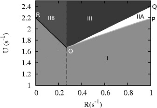
Theoretical phase diagram for the vectorial model with two ends in the variables hydrolysis rate R and on-rate U. The line OQ is obtained by setting the cap velocity equal to zero, and the line OP is given by the condition v_IIA = 0 where v_IIA is the velocity in phase IIA calculated in Eq. 2. Similarly, the line OR is given by the condition v_IIB = 0, where v_IIB is the velocity in phase IIB given in Eq. 5.

This phase diagram can be understood from the random walk representation of Fig. 1. The velocity of the random walker in the bulk has components v_n = (R – W_D^–)d along the x axis and v_k = (U – W_T⁺ – R)d along the y axis, where d is the subunit size. Depending on the signs of these quantities, four cases emerge. If v_n > 0 and v_k > 0, both the filament and cap length increase without bound; this corresponds to phase III. If v_n < 0 and v_k < 0, both the filament and cap length stay bounded and we have phase I. If v_n > 0 and v_k < 0, the cap length remains constant in time, but the rest of the filament made of D subunits can be either bounded (then we are again in phase I) or unbounded (and we are in phase IIA). Similarly, if v_n < 0 and v_k > 0, the length of the region of D subunits at the pointed end remain constant in time, but the region of T subunits can be either bounded (phase I) or unbounded (phase IIB). In phase IIA, the probability of finding a nonzero cap,

$$q=\frac{U}{W_{\text{T}}^{+}+R},$$ (1)

is finite, and the average filament velocity is (see the Appendix)

$$v_{\text{IIA}}=\left[U-W_{\text{T}}^{+}q-W_{\text{D}}^{+}\left(1-q\right)-W_{\text{D}}^{-}\right]d\text{.}$$ (2)

At the critical concentration c = c_A, v_IIA = 0 and this marks the boundary to phase I. We find that

$$c_{\text{A}}=\frac{\left(W_{\text{D}}^{+}+W_{\text{D}}^{-}\right)}{k_0}\left(\frac{W_{\text{T}}^{+}+R}{W_{\text{D}}^{+}+R}\right),$$ (3)

which is always larger than the critical concentration of the barbed end alone. In region III, the velocity is still given by

$$v_{\text{III}}=\left[U-W_{\text{T}}^{+}\right]d\text{.}$$ (4)

Similarly, in phase IIB, the probability of finding a nonzero region of D-subunits $\tilde{q}=R/W_{\text{D}}^{-}$ is finite, and the average filament velocity is

$$v_{\text{IIB}}=\left[U-W_{\text{T}}^{+}-W_{\text{T}}^{-}\left(1-\tilde{q}\right)-W_{\text{D}}^{-}\tilde{q}\right]d,$$ (5)

which vanishes when c = c_B at the boundary with phase I, with

$$c_{\text{B}}=\frac{1}{k_0}\left[\left(W_{\text{T}}^{-}-W_{\text{D}}^{-}\right)\left(1-\frac{R}{W_{\text{D}}^{-}}\right)+\left(W_{\text{T}}^{+}+W_{\text{D}}^{-}\right)\right]\text{.}$$ (6)

Note that W_T^– does not enter in v_IIA, because the hydrolyzed part of the filament is always infinitely large in this case, in contrast to the case of v_IIB, which depends on both W_T^– and W_D^–. Note also that the velocity v_IIA and v_IIB are sums of a contribution due to the barbed end and a contribution due to the pointed end. This is because in all growing phases, the filament is infinitely long in the steady state, and therefore the dynamics of each end is independent of the other. In Fig. 4, all the velocities computed from Eqs. 2, 4, and 5 have been plotted.

Figure 4.

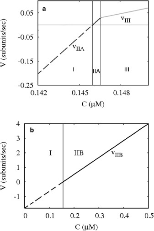
Filament velocity v versus concentration of free monomers C for the vectorial model with two active ends. (a) Case R > W_D^– for R = 0.3. In regions I and IIA, v = v_IIA, where v_IIA is given by Eq. 2. In region III, v = v_III, where the velocity is that of Eq. 4. (b) Case R < W_D^– for R = 0.2. Here v = v_IIB where v_IIB is given by Eq. 5.

Length fluctuations of the filament are characterized by a diffusion coefficient which is defined in the Appendix. Because the dynamics of each end is independent in phase IIA, the diffusion coefficient of this phase D_IIA is the sum of a contribution from the barbed end and another from the pointed end. From Ranjith et al. (11) we obtain

$$D_{\text{IIA}}=\frac{d^2}{2}\left[U+W_{\text{T}}^{+}q+W_{\text{D}}^{+}\left(1-q\right)+\frac{2\left(W_{\text{D}}^{+}-W_{\text{T}}^{+}\right)\left(U+W_{\text{D}}^{+}q\right)}{W_{\text{T}}^{+}+R}+W_{\text{D}}^{-}\right],$$ (7)

where (W_D^–d²)/2 is the contribution of the diffusion coefficient due to the pointed end. A similar expression can be obtained for D_IIB.

On the boundary lines c = c_A and c = c_B, the average filament velocity vanishes. At this point, the addition of subunits at the barbed-end exactly compensates the loss of subunits at the pointed-end. Such a state is well known in the literature as treadmilling (21). There, the length diverges as –D_IIA/v_IIA near c = c_A and similarly as –D_IIB/v_IIB near c = c_B as shown in Fig. 5, where D_IIA and D_IIB are diffusion coefficient in phases IIA and IIB. That divergence is a consequence of the assumption that the filament is in contact with a reservoir of monomers; in experimental conditions, the maximum length is fixed by the total amount of monomers. In the bulk of phase I, the average velocity is zero due to a succession of collapses and nucleations of a new filament. In this phase, there is a steady state with a well-defined treadmilling average length.

Figure 5.

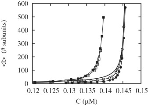
Average length as function of concentration. (Solid circles) W_T^– = 0.8 and W_D^– = 0.27; (open circles) W_T^– = 0 and W_D^– = 0.27; (open squares) W_T^– = 0.8 and W_D^– = 0; and (solid squares) W_T^– = 0 and W_D^– = 0. The rates which are not specified here are given in Table 1. The solid line is D_IIA(c = c_A)/v_IIA.

As mentioned above, because the two ends are far from each other in the growing phases, they can be treated independently. In the phase of bounded growth (phase I), however, where the filament length reaches zero occasionally, the two ends are interacting strongly. For this reason, a precise description of the phase of bounded growth is more difficult (see the Appendix). Because of this, we have computed numerically the average length in Fig. 5 as function of the free monomer concentration. In this figure, we compare the case of the filament with two ends to the case with one end only. We see that there is a small increase in the critical concentration where the length diverges and a corresponding lowering of the average length due to the inclusion of both ends in the model. This effect is correctly captured by Eqs. 3–6. Note that although there are large length fluctuations in phase I, the diffusion coefficient D_I as defined in the Appendix is zero in phase I, because these fluctuations do not depend on time.

Hydrolysis within the Filament: A Vectorial or Random Process?

Growth velocity

As explained earlier, we have used a simplified model for hydrolysis (12), in which the first step of hydrolysis is absent. The only remaining step, the phosphate release, is assumed to be a vectorial process. In the following, we keep this assumption, but we compare the two limiting mechanisms for the phosphate release, namely the vectorial and the random processes. All the rates have the same meaning for both models, except for the hydrolysis rate which is denoted R in the vectorial model and r in the random model.

We have compared experimental data from Carlier et al. (22) together with the two theoretical models, vectorial and random. Both models successfully account for the observed sharp bend in the velocity versus concentration plots observed near the critical concentration as shown in Figs. 6 and 7. Below the critical concentration, the velocity is negative for depolymerizing filaments and it is the velocity of phase II, as phase II extends transiently below the critical concentration.

Figure 6.

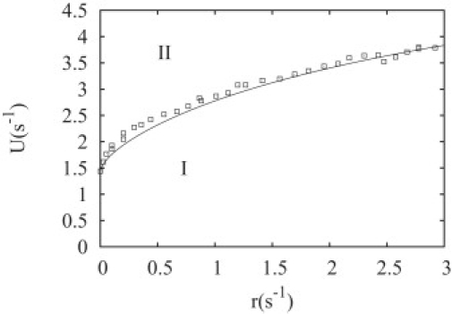
Phase diagram of the random hydrolysis in the coordinate on-rate U versus hydrolysis rate r (per site). The symbols have been obtained from Monte Carlo simulations, whereas the solid line is the mean-field theory of the Appendix. For r = 0, we recover the value of U corresponding to the critical concentration of the vectorial model.

Figure 7.

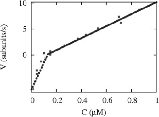
Velocity versus free monomer concentration. The square symbols are experimental data of Carlier et al. (22), which were themselves taken from Carlsson (32); the solid lines is the velocity for the random model as calculated from the theory presented in the Appendix; and the plus symbols indicate the velocity for the vectorial model using rates in Table 1, except for R = 0.12 s⁻¹ and W_D⁺ = 6.7 s⁻¹.

Note that the velocities of both models superimpose, which means that bulk velocity measurements do not allow us to discriminate between these models. Irrespective of the actual hydrolysis (phosphate release) mechanism, a fit of this data provides a bound on the value of the hydrolysis rate in the vectorial model R, which is not accurately determined experimentally. This parameter, was roughly estimated in Stukalin and Kolomeisky (12) to be 0.3 s⁻¹ based on measurements of Pi release by Melki et al. (23). The measured hydrolysis rate was multiplied by a typical length to get the estimate for R. Our fit of the data of Pantaloni et al. (24) gives R = 0.1 ± 0.12 s⁻¹. This is the value which we have used for later comparison.

In Fig. 6, the phase diagram of the random hydrolysis model is shown. This phase diagram has only two phases in contrast to the vectorial case, because it can be shown that the average of the total amount of ATP subunits 〈k〉 is always bounded in the random model. Thus phase III is absent in the random model. In the Appendix, we present details about the derivation of the mean-field equations for the random model (25,26). An analytical expression for the phase boundary between phase I and II is obtained, which corresponds to the solid line in Fig. 6 and which agrees well with the Monte Carlo simulations.

Length diffusivity

Length fluctuations are quantified by the length diffusivity, also called diffusion coefficient D, which is defined in Eq. 18. The length diffusivity of single filaments has been measured using TIRF microscopy by two groups (27,28). Both groups reported rather high values, of ∼30 monomer²/s. This value is high when thinking in terms of the rates of assembly and disassembly measured in bulk (29,30). From such bulk measurements, one could have expected a length diffusivity at the critical concentration of 1 monomer²/s, an order-of-magnitude smaller than observed in single filament experiments.

Several studies have been carried out to explain this discrepancy: Vavylonis et al. (7) computed the diffusion coefficient D as a function of ATP monomer concentration and found that D is peaked just below the critical concentration and its maximum is comparable to the value observed in experiments (≈30 monomer²/s). Stukalin et al. (12) obtained from an analytical model the same large values for D (≈30 monomer²/s) just above the critical concentration. Recently, Fass et al. (20) studied the length diffusivity numerically taking into account filament fragmentation and annealing, within the vectorial model. They found that high length diffusivity at the critical concentration cannot be explained by fragmentation and annealing events unless both fragmentation and annealing rates are much greater than previously thought. In the limit where their fragmentation rate goes to zero, they recover the results of Vavylonis et al. (7). Others have proposed that the discrepancy in diffusivity may be related to experimental errors in the length of the filament due to out-of-plane bending of the filaments (M. F. Carlier, CNRS, France, private communication, 2009).

According to Stukalin et al. (12) and Vavylonis et al. (7), the large length diffusivity observed in experiments results from dynamic instability-like fluctuations of the cap. It is important to point out that both articles make very different assumptions: the first one describes hydrolysis as a single step corresponding to Pi release with the vectorial mechanism; the second one describes both steps as random processes.

We have shown in Fig. 8 the concentration dependence of D for the vectorial model using analytical expressions provided in the Appendix and similar to that of Ranjith et al. (11) and Stukalin and Kolomeisky (12). In this figure, the critical concentration defined as the boundary between phases I and II almost coincides with the concentration at the boundary between phases II and III; both are of the order of 0.14 μM. Above this value, D is indeed small—the expected estimate of 1 monomer²/s is indeed recovered there because the contribution of hydrolysis is negligible. Near the critical concentration, however, the fluctuations are much larger, essentially for the same reason that leads to large fluctuations near critical points in condensed matter systems (31). Here, hydrolysis, known to destabilize filaments, has a larger effect. It leads to large fluctuations of the cap, and ultimately to a large length diffusivity. Note that the region below the critical concentration corresponds to the transient extension of phase II discussed in the previous section. If the fluctuations were probed there for a very long time, one would find D = D_I = 0, characteristic of phase I.

Figure 8.

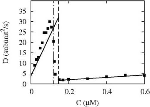
Diffusion coefficient as function of the monomer concentration for the random and vectorial model of hydrolysis. The data points are the prediction for the random model of hydrolysis whereas the solid lines are the predictions for the vectorial model. The dashed (respectively, dash-dotted) vertical line represents the critical concentration for the vectorial (respectively, random) model.

In Fig. 8, we have compared these analytical results obtained for the vectorial model with numerical results obtained for the random model. In the random model, we use Monte Carlo simulations to calculate a time-dependent diffusion coefficient D(t), defined as

$$D\left(t\right)=\frac{1}{2}\frac{\text{d}}{\text{dt}}\left(\langle l^2\rangle -{\langle l\rangle }^2\right)\text{.}$$

For concentrations larger than the critical concentration, the initial condition is l(t = 0) = 0, whereas for concentrations smaller than the critical concentration, the initial condition was a very long filament (l(t = 0) > 10⁶ subunits) with all subunits in the hydrolyzed state. On a large time window, we find that D(t) is approximately time-independent, and we interpret that value as the length diffusivity of the random model. Our results fully agree with that of Vavylonis et al. (7), and with that of Fass et al. (20) in the limit of zero fragmentation rate. The length diffusivity indeed reaches a maximum of ∼30 monomer²/s below the critical concentration. As shown in that figure, there is only a small difference of length diffusivity in the vectorial case as compared to the random case: the maximum of the curve for the random model occurs at a smaller concentration than in the vectorial model. The fact that we are able to reproduce a similar curve to that shown in the literature (7,20) justifies our simplifying assumption of describing the hydrolysis as a single step associated with the release of phosphate (rather than taking into account the two steps as performed in (7,20)). More importantly, it confirms the idea that the length diffusivity of actin, near critical concentration, is dominated by a process similar to the dynamic instability, which is essentially captured by the vectorial model.

To make further progress, it would be very useful to reproduce experiments similar to those of Fujiwara et al. (27), on single filaments for various monomer concentrations, to confirm the scenario presented above for the length fluctuations of actin. Given that the predictions of the random and vectorial model are rather close to each other as shown in Fig. 8, it is likely that it will be difficult to distinguish between these models from measurements of the concentration dependence of the length diffusivity. The length diffusivities of the two models are very close to each other because a very small value of the hydrolysis rate r (as estimated from experiments) has been used. We have observed that if this parameter had a larger value than referenced here, the predictions of the vectorial and random model would differ far more.

Dynamics of the Filament in Transient Regimes

Because it appears difficult to distinguish the vectorial from the random model using measurements of growth velocity or length diffusivity, one can turn to an analysis of the dynamics of the filament length in polymerization (27) or in depolymerization (5,10) to discriminate between the two models. Here, we focus on the dynamics of polymerization of a single filament, in the presence of a constraint of conservation of the total number of subunits (free+polymerized). This constraint leads to a steady state with a constant average length for the filament. We compare the time it takes for the filament to be fully hydrolyzed to the time that it takes to reach the steady-state length. We also discuss the corresponding length fluctuations as a function of time. We argue that both measurements (the lag time of hydrolysis and the time-resolved fluctuations) can distinguish between the two mechanisms of hydrolysis.

In Fig. 9, we show the filament length as well as its variance, as a function of time, for both vectorial and random models. Using Monte Carlo simulations we computed l(t), starting from l(t = 0) = 0, for 1000 different realizations and calculated σ²(t) = 〈l²〉 – 〈l〉². Concerning the lag time of hydrolysis, we have observed that in simulations of the vectorial model, the filament typically reaches its steady-state length long before it has been completely hydrolyzed. The time when this happens corresponds to the point where the two curves meet in Fig. 9 a. This characteristic time, because only one end is involved, is t_H ≃ 〈l〉/R, where R is the hydrolysis rate in the vectorial model (11). From the figure we find that t_H ≃ 3500/0.3 ≃ 11,000 s ≃ 180 min (with R ≃ 0.3, which is much longer than the typical time to reach the steady state t_SS ≃ 〈l〉/v ≃ 3500/(11.6 × 0.7 − 1.4) = 520 s. In contrast to this, in the random model, the time for completion of hydrolysis is comparable to the time to reach steady state (see Fig. 9 b) as both the filament and the ADP part have similar growth dynamics.

Figure 9.

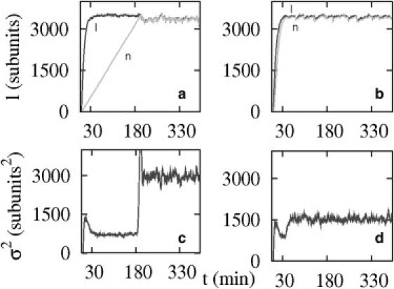
(a and b) Total filament length (denoted l, solid), and total amount of hydrolyzed subunits (denoted n, shaded) as function of time for the case of vectorial hydrolysis (left panel) and random hydrolysis (right panel) (the total concentration of subunits c_T = 0.7 μM; one filament in a volume of 10 (μm)³). Note that the point where the two curves meet in the random hydrolysis model occurs much earlier compared to the case of vectorial hydrolysis (≈10,000 s). (c and d) The variance (σ² = 〈l²〉 – 〈l〉²) as a function of time is plotted for the vectorial model and random model, respectively.

In practice, this lag time of hydrolysis may be difficult to measure on single filaments as the ATP subunits and ADP subunits cannot be distinguished easily experimentally. In view of the previous section, on the role of ATP hydrolysis in length diffusivity, we suggest to study instead the length fluctuations of the filament as a function of time. Such a quantity is accessible from image analysis of single filaments with TIRF, for instance. We have simulated the variance of the length fluctuations σ(t)² = 〈l(t)²〉 – 〈l(t)〉² as function of time, for the vectorial model and random model, as shown in Fig. 9, c and d, respectively. At early times, this variance is linear in time, and the slope corresponds to the length diffusivity discussed in previous section, because the constraint of conservation of monomers plays no role at short times. Once the steady state has been reached, we find that the variance of the vectorial model shows a sharp increase when t ≥ t_H, whereas the variance of the random model shows no significant change. The approximately constant variance of the random model is intermediate between the variance of the vectorial model before and after the jump.

Thus, contrary to velocity and length diffusivity measurements, an analysis of either the lag time of hydrolysis or of the time dependence of the length fluctuations provide a direct signature of the underlying mechanism of hydrolysis.

Conclusion

In this article, we have analyzed several aspects of the dynamics of a single actin filament. Many results discussed above could be extended, with the necessary changes having been made, to the case of microtubules.

We have constructed a phase diagram, which summarizes all the possible dynamical phases of an actin filament with two active ends and vectorial hydrolysis in its inside. We have found that quantities like the filament velocity and the length diffusivity show similar behavior for both vectorial and random models of hydrolysis. We propose that measuring the length fluctuations of a single filament as a function of time can distinguish between the two models for hydrolysis (or to be more precise, to the step of phosphate release). Although more experimental and theoretical work are needed, investigations of the dynamics of the length of single filaments during polymerization (27) and during depolymerization (5,10) indicate that the mechanism of phosphate release is not purely vectorial or purely random, but rather probably intermediate between these two limiting cases.

We hope that our study will contribute to the understanding of the nonequilibrium self-assembly of actin/microtubule filaments.

Appendix

Equations of the vectorial model with two ends

Let P(n, k, t) be the probability of having n hydrolyzed ADP subunits and k unhydrolyzed ATP subunits at time t, such that l = (n + k)d is the total length of the filament. It obeys the following master equation: For k > 0 and n > 0, we have

$$\frac{dP\left(n,k,t\right)}{dt}=UP\left(n,k-1,t\right)+W_{\text{T}}^{+}P\left(n,k+1,t\right)+RP\left(n-1,k+1,t\right)+W_{\text{D}}^{-}P\left(n+1,k\right)-\left(U+W_{\text{T}}^{+}+R+W_{\text{D}}^{-}\right)P\left(n,k,t\right)\text{.}$$ (8)

For k > 0 and n = 0,

$$\frac{dP\left(0,k,t\right)}{dt}=UP\left(0,k-1,t\right)+\left(W_{\text{T}}^{+}+W_{\text{T}}^{-}\right)P\left(0,k+1,t\right)+W_{\text{D}}^{-}P\left(1,k\right)-\left(U+W_{\text{T}}^{+}+W_{\text{T}}^{-}+R\right)P\left(0,k,t\right)\text{.}$$ (9)

For k = 0 and n ≥ 1, we have

$$\frac{dP\left(n,0,t\right)}{dt}=\left(W_{\text{D}}^{+}+W_{\text{D}}^{-}\right)P\left(n+1,0,t\right)+W_{\text{T}}^{+}P\left(n,1,t\right)+RP\left(n-1,1,t\right)-\left(U+W_{\text{D}}^{+}+W_{\text{D}}^{-}\right)P\left(n,0,t\right)\text{.}$$ (10)

If k = 0 and n = 0, we have

$$\frac{dP\left(0,0,t\right)}{dt}=\left(W_{\text{T}}^{+}+W_{\text{T}}^{-}\right)P\left(0,1,t\right)+\left(W_{\text{D}}^{+}+W_{\text{D}}^{-}\right)P\left(1,0,t\right)-UP\left(0,0,t\right)\text{.}$$ (11)

We define the following generating functions

$$G\left(x,y,t\right)=\sum _{\text{n}\ge 0}\sum _{\text{k}\ge 0}P\left(n,k,t\right)x^{\text{n}}{y}^{\text{k}},$$ (12)

$$F_{\text{k}}\left(x,t\right)=\sum _{\text{n}\ge 0}P\left(n,k,t\right)x^{\text{n}},$$ (13)

$$H_{\text{n}}\left(y,t\right)=\sum _{\text{k}\ge 0}P\left(n,k,t\right)y^{\text{k}}\text{.}$$ (14)

Normalization imposes that at all times t,

$$G\left(1,1,t\right)=\sum _{\text{n}=0}^{\infty }\sum _{\text{k}=0}^{\infty }P\left(n,k,t\right)=1.$$ (15)

Using Eqs. 8–11, we obtain the evolution equation for G(x, y, t),

$$\begin{array}{l}\frac{dG(x,y,t)}{dt}=\left[U\left(y-1\right)+W_{\text{T}}^{+}\left(\frac{1}{y}-1\right)+R\left(\frac{x}{y}-1\right)+W_{\text{D}}^{-}\left(\frac{1}{x}-1\right)\right]G\left(x,y,t\right)\\ -\left[W_{\text{T}}^{+}\left(\frac{1}{y}-1\right)+R\left(\frac{x}{y}-1\right)+W_{\text{D}}^{+}\left(1-\frac{1}{x}\right)\right]F_0\left(x,t\right)\\ -\left[W_{\text{D}}^{-}\left(\frac{1}{x}-1\right)+W_{\text{T}}^{-}\left(1-\frac{1}{y}\right)\right]H_0\left(y,t\right)\\ -\left[W_{\text{D}}^{+}\left(\frac{1}{x}-1\right)-W_{\text{T}}^{-}\left(1-\frac{1}{y}\right)\right]P\left(0,0,t\right)\text{.}\end{array}$$ (16)

From G(x, y, t), the following quantities can be obtained: the velocity of the filament, which is

$$v=\underset{\text{t}\to \infty }{\lim }\frac{d\langle l\rangle }{dt}=d\underset{\text{t}\to \infty }{\lim }\frac{\partial }{\partial x}{\left(\frac{dG\left(x,x,t\right)}{dt}\right)}_{\text{x}=1},$$ (17)

and the diffusion coefficient characterizing filament length fluctuations,

$$\begin{array}{l}D=\underset{\text{t}\to \infty }{\lim }\frac{1}{2}\frac{d}{dt}\left(\langle l^2\rangle -{\langle l\rangle }^2\right)\\ =d^2\underset{\text{t}\to \infty }{\lim }[\frac{1}{2}\frac{{\partial }^2}{\partial x^2}\left(\frac{dG(x,x,t)}{dt}\right)+\frac{1}{2}\frac{\partial }{\partial x}\left(\frac{dG(x,x,t)}{dt}\right)\\ -{\left(\frac{\partial G(x,x,t)}{\partial x}\right)\frac{\partial }{\partial x}\left(\frac{dG(x,x,t)}{dt}\right)]}_{\text{x}=1}\text{.}\end{array}$$ (18)

The average cap velocity is

$$J=d\underset{\text{t}\to \infty }{\lim }\frac{d\langle k\rangle }{dt}=d\underset{\text{t}\to \infty }{\lim }\frac{\partial }{\partial y}{\left(\frac{dG(1,y,t)}{dt}\right)}_{\text{y}=1},$$ (19)

and the diffusion coefficient characterizing the fluctuations of the cap is

$$\begin{array}{l}{D}_{\text{c}}=d^2\underset{\text{t}\to \infty }{\lim }\frac{1}{2}\frac{d}{dt}\left(\langle k^2\rangle -{\langle k\rangle }^2\right)\\ =d^2\underset{\text{t}\to \infty }{\lim }[\frac{1}{2}\frac{{\partial }^2}{\partial y^2}\left(\frac{dG(1,y,t)}{dt}\right)+\frac{1}{2}\frac{\partial }{\partial y}\left(\frac{dG(1,y,t)}{dt}\right)\\ -{\left(\frac{\partial G(1,y,t)}{\partial y}\right)\frac{\partial }{\partial y}\left(\frac{dG(1,y,t)}{dt}\right)]}_{\text{y}=1}\text{.}\end{array}$$ (20)

Phase diagram and average length in the bounded phase

To construct the phase diagram, we first focus on steady-states solutions of Eq. 16, which are such that dG(x, y, t)/dt = 0. The obtained equation for G(x, y) involves the following time-independent quantities,

$$F_0\left(x\right)=G\left(x,0\right)=\sum _{\text{n}\ge 0}P\left(n,0\right)x^{\text{n}},$$ (21)

$$H_0\left(y\right)=G\left(0,y\right)=\sum _{\text{k}\ge 0}P\left(0,k\right)y^{\text{k}},$$ (22)

$$P\left(0,0\right)=F_0\left(0\right)=H_0\left(0\right)=G\left(0,0\right),$$ (23)

which are coupled back to G(x, y).

Progress can be made by considering two particular cases for x = 1 and y = 1 of this expression for G(x, y). This leads to

$$R-W_{\text{T}}^{-}=F_0\left(1\right)\left(R+W_{\text{D}}^{+}\right)-W_{\text{D}}^{-}{H}_0\left(1\right)-P\left(0,0\right)W_{\text{T}}^{+},$$ (24)

$$U-R-W_{\text{T}}^{+}=F_0\left(1\right)\left(R+W_{\text{D}}^{+}\right)+W_{\text{T}}^{-}{H}_0\left(1\right)-P\left(0,0\right)W_{\text{T}}^{-}\text{.}$$ (25)

These two equations involve three unknowns F₀(1): the probability that the cap is zero, H₀(1): the probability that the D part of the filament is zero, and P(0, 0): the probability that the filament is in the state of monomers. Note that P(0, 0) = 0 in phases of unbounded growth whereas P(0, 0) > 0 in the phase of bounded growth.

In the random walk representation of Fig. 1, the velocity of the random walker in the bulk has components v_n = (R – W_D^–)d along the x axis and v_k = (U – W_T⁺ – R)d along the y axis. Depending on the signs of these quantities, four cases emerge. If v_n > 0 and v_k > 0, both the filament and cap length increase without bound (phase III), which means that F₀(1) = H₀(1) = P(0, 0) = 0. If v_n < 0 and v_k < 0, both the filament and cap length stay bounded (phase I) and F₀(1) > 0, H₀(1) > 0 and P(0, 0) > 0.

If v_n > 0 and v_k < 0, the cap length remains constant in time, which means F₀(1) > 0, but the rest of the filament made of D subunits can be either bounded (for H₀(1) = P(0, 0) = 0, which corresponds to phase I) or unbounded (for H₀(1) = P(0, 0) > 0, which corresponds to phase IIA). When reporting the condition H₀(1) = P(0, 0) = 0 into Eqs. 24 and 25 and solving for F₀(1), one finds that the phase of bounded growth occurs when U/(R + W_T⁺) < (W_D⁺ + W_D^–)/(R + W_D⁺), and the boundary to the phase of unbounded growth corresponds to replacing the unequal sign by an equal sign.

An alternative way to find this condition is to start from the time-dependent evolution equation of G(x, y, t) of Eq. 16 and impose H₀(y, t) = P(0, 0, t) = 0. We end up with two coupled dynamical equations for F₀(x, t) and G(x, y, t). The way to obtain the velocity and diffusion coefficient in phase IIA from these equations is explained in detail in the Appendix of Ranjith et al. (11). The result is the expression of v_IIA given in Eq. 2, and the expression of D_IIA of Eq. 7. As expected, the condition that marks the boundary between phase IIA and phase I corresponds to v_IIA = 0.

Similarly, if v_n < 0 and v_k > 0, the length of the region of D subunits at the pointed end remains constant in time, and the region of T subunits can be either bounded (phase I) or unbounded (phase IIB). By either method, one obtains the velocity in the phase IIB given in Eq. 5, and the condition that marks the boundary to phase I, which corresponds to v_IIB = 0.

In Ranjith et al. (11), an explicit expression for the average length in the phase of bounded growth was obtained by a method of cancellation of poles of G(x, y). Unfortunately, this method does not allow us to derive the expression of G(x, y) here, because the rates W_T^– ≠ 0 and W_D^– ≠ 0 lead to an additional unknown H₀(y, t) in Eq. 16, which makes the problem much more difficult to solve. For this reason, we could not derive an explicit expression for the average length in this case, and we investigated this quantity only numerically.

Mean-field equations of the random model

We explain in this Appendix how the velocity of the filament in the random model is obtained from a mean-field approach. This Appendix is provided mainly for pedagogical reasons, since the solution has already appeared in Stukalin and Kolomeisky (12) and Keiser et al. (26). For simplicity, we focus on the case where growth and shrinking occur only from one end, which we number as the first site i = 1. We use the same notations for the rates as in the vectorial model except for the hydrolysis rate, which is denoted r in the random model. For a given configuration, we introduce for each subunit i inside the filament an occupation number τ_i, such that τ_i = 1 if the subunit binds ATP and τ_i = 0 otherwise. In the reference frame associated with the end of the filament, the equations for the average occupation number are

$$\frac{d\langle {\tau }_1\rangle }{dt}=U\left(1-\langle {\tau }_1\rangle \right)-W_{\text{T}}\langle {\tau }_1\left(1-{\tau }_2\right)\rangle +W_{\text{D}}\langle {\tau }_2\left(1-{\tau }_1\right)\rangle -r\langle {\tau }_1\rangle ,$$ (26)

$$\frac{d\langle {\tau }_{\text{i}}\rangle }{dt}=U\left(\langle {\tau }_{\text{i}-1}\left(1-{\tau }_{\text{i}}\right)\rangle -\langle {\tau }_{\text{i}}\left(1-{\tau }_{\text{i}-1}\right)\rangle \right)+W_{\text{T}}\langle {\tau }_1\left[\left(1-{\tau }_{\text{i}}\right){\tau }_{\text{i}+1}-{\tau }_{\text{i}}\left(1-{\tau }_{\text{i}+1}\right)\right]\rangle +W_{\text{D}}\langle \left(1-{\tau }_1\right)\left[\left(1-{\tau }_{\text{i}}\right){\tau }_{\text{i}+1}-{\tau }_{\text{i}}\left(1-{\tau }_{\text{i}+1}\right)\right]\rangle -r\langle {\tau }_{\text{i}}\rangle \text{.}$$ (27)

In a mean-field approach, the effect of correlations 〈τ_iτ_j〉 are neglected, i.e., these correlations are replaced by 〈τ_i〉〈τ_j〉 (and similarly for averages of product of three occupation numbers). At steady state, the left-hand sides of Eqs. 26 and 27 are both zero, which leads to recursion relations for the 〈τ_i〉. Note that 〈τ_i〉 is denoted as a_i in Keiser et al. (26) and as P_i in Stukalin and Kolomeisky (12). We still denote 〈τ₁〉 = q, because it represents the probability that the terminal unit binds ATP. It is the analog of the parameter defined in Eq. 1 for the vectorial model, which is now a more complicated function of the rates. The recursion relations have a solution of the form for i ≥ 1,

$$\frac{\langle {\tau }_{\text{i}+1}\rangle }{\langle {\tau }_{\text{i}}\rangle }=\frac{U-q\left(W_{\text{T}}+r\right)}{U-q{W}_{\text{T}}}\text{.}$$ (28)

Combining Eqs. 26–28, one obtains the following cubic equation for q:

$$\left(W_{\text{T}}+r\right)\left(W_{\text{T}}-W_{\text{D}}\right)q^3+(U{W}_{\text{D}}-2U{W}_{\text{T}}+W_{\text{D}}{W}_{\text{T}}+W_{\text{D}}r-W_{\text{T}}\text{r}-W_{\text{T}}^2)q^2+U\left(U-W_{\text{D}}+2W_{\text{T}}+r\right)q-U^2=0.$$ (29)

This cubic equation has three solutions, but only one solution is such that 0 ≤ q ≤ 1. The rate of elongation of the filament can be obtained by reporting that solution into

$$v=t\to \infty \frac{d\langle l\rangle }{dt}=\left[U-W_{\text{T}}q-W_{\text{D}}\left(1-q\right)\right]d\text{.}$$ (30)

In Fig. 7, this velocity v is shown as function of the concentration of free monomers. For low values of r, the velocity rates of the random and vectorial model are identical, because as r is increased the velocity of the random model starts to deviate from the curve of the vectorial model. By imposing the condition v = 0, one obtains the phase boundary shown in the solid line in Fig. 6.

References

- 1.Howard J. Sinauer; Sunderland, MA: 2001. Mechanics of Motor Proteins and the Cytoskeleton. [Google Scholar]
- 2.Fujiwara I., Vavylonis D., Pollard T.D. Polymerization kinetics of ADP- and ADP-Pi-actin determined by fluorescence microscopy. Proc. Natl. Acad. Sci. USA. 2007;104:8827–8832. doi: 10.1073/pnas.0702510104. [DOI] [PMC free article] [PubMed] [Google Scholar]
- 3.Phillips R., Kondev J., Theriot J. 1st Ed. Garland Science; New York: 2008. Physical Biology of the Cell. [Google Scholar]
- 4.Pieper U., Wegner A. The end of a polymerizing actin filament contains numerous ATP-Subunit segments that are disconnected by ADP-subunits resulting from ATP Hydrolysis. Biochemistry. 1996;35:4396–4402. doi: 10.1021/bi9527045. [DOI] [PubMed] [Google Scholar]
- 5.Li X., Kierfeld J., Lipowsky R. Actin polymerization and depolymerization coupled to cooperative hydrolysis. Phys. Rev. Lett. 2009;103:048102. doi: 10.1103/PhysRevLett.103.048102. [DOI] [PubMed] [Google Scholar]
- 6.Dimitrov A., Quesnoit M., Perez F. Detection of GTP-tubulin conformation in vivo reveals a role for GTP remnants in microtubule rescues. Science. 2008;322:1353–1356. doi: 10.1126/science.1165401. [DOI] [PubMed] [Google Scholar]
- 7.Vavylonis D., Yang Q., O'Shaughnessy B. Actin polymerization kinetics, cap structure, and fluctuations. Proc. Natl. Acad. Sci. USA. 2005;102:8543–8548. doi: 10.1073/pnas.0501435102. [DOI] [PMC free article] [PubMed] [Google Scholar]
- 8.Bindschadler M., Osborn E.A., McGrath J.L. A mechanistic model of the actin cycle. Biophys. J. 2004;86:2720–2739. doi: 10.1016/S0006-3495(04)74326-X. [DOI] [PMC free article] [PubMed] [Google Scholar]
- 9.Brooks F.J., Carlsson A.E. Actin polymerization overshoots and ATP hydrolysis as assayed by pyrene fluorescence. Biophys. J. 2008;95:1050–1062. doi: 10.1529/biophysj.107.123125. [DOI] [PMC free article] [PubMed] [Google Scholar]
- 10.Kueh H.Y., Brieher W.M., Mitchison T.J. Dynamic stabilization of actin filaments. Proc. Natl. Acad. Sci. USA. 2008;105:16531–16536. doi: 10.1073/pnas.0807394105. [DOI] [PMC free article] [PubMed] [Google Scholar]
- 11.Ranjith P., Lacoste D., Joanny J.F. Nonequilibrium self-assembly of a filament coupled to ATP/GTP hydrolysis. Biophys. J. 2009;96:2146–2159. doi: 10.1016/j.bpj.2008.12.3920. [DOI] [PMC free article] [PubMed] [Google Scholar]
- 12.Stukalin E.B., Kolomeisky A.B. ATP hydrolysis stimulates large length fluctuations in single actin filaments. Biophys. J. 2006;90:2673–2685. doi: 10.1529/biophysj.105.074211. [DOI] [PMC free article] [PubMed] [Google Scholar]
- 13.Dogterom M., Leibler S. Physical aspects of the growth and regulation of microtubule structures. Phys. Rev. Lett. 1993;70:1347–1350. doi: 10.1103/PhysRevLett.70.1347. [DOI] [PubMed] [Google Scholar]
- 14.Flyvbjerg H., Holy T.E., Leibler S. Microtubule dynamics: caps, catastrophes, and coupled hydrolysis. Phys. Rev. E Stat. Phys. Plasmas Fluids Relat. Interdiscip. Topics. 1996;54:5538–5560. doi: 10.1103/physreve.54.5538. [DOI] [PubMed] [Google Scholar]
- 15.Zong C., Lu T., Wolynes P.G. Nonequilibrium self-assembly of linear fibers: microscopic treatment of growth, decay, catastrophe and rescue. Phys. Biol. 2006;3:83–92. doi: 10.1088/1478-3975/3/1/009. [DOI] [PubMed] [Google Scholar]
- 16.Antal T., Krapivsky P.L., Chakraborty B. Dynamics of an idealized model of microtubule growth and catastrophe. Phys. Rev. E Stat. Nonlin. Soft Matter Phys. 2007;76:041907. doi: 10.1103/PhysRevE.76.041907. [DOI] [PMC free article] [PubMed] [Google Scholar]
- 17.Antal T., Krapivsky P.L., Redner S. Dynamics of microtubule instabilities. J. Stat. Mech. 2007 doi: 10.1088/1742-5468/2007/05/L05004. L05004. [DOI] [PMC free article] [PubMed] [Google Scholar]
- 18.Sumedha M., Hagan F., Chakraborty B. Role of GTP remnants in microtubule dynamics. arXiv. 2009 0908.1199:1–4. [Google Scholar]
- 19.Carlier M.F., Pantaloni D. Direct evidence for ADP-Pi-F-actin as the major intermediate in ATP-actin polymerization. Rate of dissociation of Pi from actin filaments. Biochemistry. 1986;25:7789–7792. doi: 10.1021/bi00372a001. [DOI] [PubMed] [Google Scholar]
- 20.Fass J., Pak C., Mogilner A. Stochastic simulation of actin dynamics reveals the role of annealing and fragmentation. J. Theor. Biol. 2008;252:173–183. doi: 10.1016/j.jtbi.2008.01.001. [DOI] [PMC free article] [PubMed] [Google Scholar]
- 21.Hill T. Springer-Verlag; New York: 1989. Free Energy Transduction and Biochemical Cycle Kinetics. [Google Scholar]
- 22.Carlier M.-F., Pantaloni D., Korn E.D. The effects of Mg2+ at the high-affinity and low-affinity sites on the polymerization of actin and associated ATP hydrolysis. J. Biol. Chem. 1986;261:10785–10792. [PubMed] [Google Scholar]
- 23.Melki R., Fievez S., Carlier M.F. Continuous monitoring of Pi release following nucleotide hydrolysis in actin or tubulin assembly using 2-amino-6-mercapto-7-methylpurine ribonucleoside and purine-nucleoside phosphorylase as an enzyme-linked assay. Biochemistry. 1996;35:12038–12045. doi: 10.1021/bi961325o. [DOI] [PubMed] [Google Scholar]
- 24.Pantaloni D., Hill T.L., Korn E.D. A model for actin polymerization and the kinetic effects of ATP hydrolysis. Proc. Natl. Acad. Sci. USA. 1985;82:7207–7211. doi: 10.1073/pnas.82.21.7207. [DOI] [PMC free article] [PubMed] [Google Scholar]
- 25.Kolomeisky A.B., Fisher M.E. Force-velocity relation for growing microtubules. Biophys. J. 2001;80:149–154. doi: 10.1016/S0006-3495(01)76002-X. [DOI] [PMC free article] [PubMed] [Google Scholar]
- 26.Keiser T., Schiller A., Wegner A. Nonlinear increase of elongation rate of actin filaments with actin monomer concentration. Biochemistry. 1986;25:4899–4906. doi: 10.1021/bi00365a026. [DOI] [PubMed] [Google Scholar]
- 27.Fujiwara I., Takahashi S., Ishiwata S. Microscopic analysis of polymerization dynamics with individual actin filaments. Nat. Cell Biol. 2002;4:666–673. doi: 10.1038/ncb841. [DOI] [PubMed] [Google Scholar]
- 28.Kuhn J.R., Pollard T.D. Real-time measurements of actin filament polymerization by total internal reflection fluorescence microscopy. Biophys. J. 2005;88:1387–1402. doi: 10.1529/biophysj.104.047399. [DOI] [PMC free article] [PubMed] [Google Scholar]
- 29.Pollard T.D. Rate constants for the reactions of ATP- and ADP-actin with the ends of actin filaments. J. Cell Biol. 1986;103:2747–2754. doi: 10.1083/jcb.103.6.2747. [DOI] [PMC free article] [PubMed] [Google Scholar]
- 30.Pollard T.D., Blanchoin L., Mullins R.D. Molecular mechanisms controlling actin filament dynamics in nonmuscle cells. Annu. Rev. Biophys. Biomol. Struct. 2000;29:545–576. doi: 10.1146/annurev.biophys.29.1.545. [DOI] [PubMed] [Google Scholar]
- 31.Chaikin P.M., Lubensky T. Cambridge University Press; Cambridge, UK: 1995. Principles of Condensed Matter Physics. [Google Scholar]
- 32.Carlsson A.E. Model of reduction of actin polymerization forces by ATP hydrolysis. Phys. Biol. 2008;5:036002–036011. doi: 10.1088/1478-3975/5/3/036002. [DOI] [PubMed] [Google Scholar]