Automated clustering of probe molecules from solvent mapping of protein surfaces: New algorithms applied to hot-spot mapping and structure-based drug design

Abstract

Use of solvent-mapping, based on multiple-copy minimization (MCM) techniques, is common in structure-based drug discovery. The minima of small-molecule probes define locations for complementary interactions within a binding pocket. Here, we present improved methods for MCM. In particular, a Jarvis-Patrick method is outlined for grouping the final locations of minimized probes into physical clusters. This algorithm has been tested through a study of protein-protein interfaces, showing the process to be robust, deterministic, and fast in the mapping of protein “hot spots”. Improvements in the initial placement of probe molecules are also described. A final application to HIV-1 protease shows how our automated technique can be used to partition data too complicated to analyze by hand. These new automated methods may be easily and quickly extended to other protein systems, and our clustering methodology may be readily incorporated into other clustering packages.

Introduction

In an effort to understand protein binding and function, researchers will often create a reciprocal map of a protein surface. Multiple-copy methods (MCM) use probe molecules to define these complementary maps. These techniques flood the protein surface with hundreds of small molecule probes. The probes are then simultaneously and independently minimized to the protein's potential energy surface. Different probe molecules map out hydrophobic regions, hydrogen-bonding interactions, ion pairing, etc. Clusters of probes on the protein surface can define the most important among these interactions. However, grouping probes into clusters is not always straightforward, and yet, it is essential to mapping “hot spots” [1] and fragment-based drug design [2-4]. Despite this importance, there is little diversity in the methods used for defining clusters.

Clustering techniques

The most widely known MCM is multiple copy simultaneous search (MCSS) [5]. The applications tend to remove probes throughout the minimization process. Root-mean-square difference (RMSD)-based clustering is used at each step, and only the lowest-energy member of each cluster is retained. Additionally, an energy cutoff is used so that high-energy probes are removed throughout the minimization. In some implementations, these clusters are then ranked via energy-based techniques [6]. MCSS2PTS automates the procedure of using the MCSS method to generate pharmacophore models [7]. In doing so, it uses standard RMSD methods to cluster the minimized probes.

Many different methodologies have been used to group molecules into clusters in chemical space such as RMSD-based methods, K-means clustering [8] and Jarvis-Patrick (JP) clustering [9], but almost all MCSS-style methods have used standard RMSD techniques to cluster the probes in physical space [5, 6, 10-13]. This technique takes two forms, which we will refer to as seeded RMSD (sRMSD) and greedy RMSD (gRMSD) clustering. The sRMSD-clustering technique works as follows:

1. Choose a distance cutoff, R_max.

2. Choose any element, i, called the seed (typically, one begins with the lowest-energy element).

3. Assign all elements that are within R_max of i to a cluster and remove them from the list of elements.

4. Repeat steps 2-3 until the list is empty.

It is worth noting that mapping techniques that find a minimum energy probe and then force subsequent probes to remain outside a given RMSD cutoff effectively use a type of sRMSD clustering.

sRMSD is limited by the need to choose proper seeds. An improved approach, gRMSD clustering (also known as single-linkage clustering) works similarly but overcomes errors in poor choices for seeds:

1. Cluster elements as per sRMSD clustering.

2. If any element in one cluster is R_max of any element in another cluster, combine the two clusters.

3. Repeat step 2 until no more clusters can be combined.

An alternative, energy-based clustering technique has been implemented with MCSS [14, 15]. Although the full details of their algorithm have not been published, a basic description has been given. Probes are clustered together when they have a similar set of van der Waals contacts with the protein. Thus, each cluster is identified by a “cluster signature” listing the amino acids with which that cluster interacts. These cluster signatures typically contain between three and thirteen residues.

One notable exception to the usage of sRMSD and gRMSD techniques is SitePrint [16]. SitePrint floods a structure with small chemical probes, which are then minimized to the protein surface. The k-medoid algorithm [17] is then used to cluster the probes. For k-medoid clustering, the user pre-determines a desired number of clusters (k). This number of clusters is then selected, and a representative element is chosen for each cluster. For each cluster, the sum of the dissimilarities between the individual elements and its representative element is calculated. The clusters and representative elements are chosen in a way that minimizes the total of these sums. The representative elements are then used to define pharmacophore models.

We have chosen not to use k-medoid or k-means clustering in this work because of their need to pre-define the number of interactions in a cavity, which is not easily extended across all systems. Instead, we compare gRMSD to a new Jarvis-Patrick (JP) [9] method. Based on two user-defined parameters (J and K_min, both positive integers), JP clustering is defined as follows:

1. Make a list of each element's J nearest neighbors.

2. Two elements cluster together if

   1. they are in each other's nearest neighbor lists and

   2. they have at least K_min of their J nearest neighbors in common.

We have also found it useful to add distance constraint to focus the neighbor list. A colloquial example of JP clustering is defining two people to be in the same social circle if they are alike enough and have enough similar friends in common. JP clustering is typically applied to questions of chemical similarity, where it has been shown to be one of the best-performing algorithms [18]. There is one example of symmetry-corrected JP clustering applied to physical similarity [19, 20] where the authors used JP clustering to provide a conformational breakdown of six-membered ring compounds in the Cambridge Structural Database [21]. They found that JP clustering performed excellently. We have found no previous applications of JP clustering (symmetry-corrected or not) to MCM or to the study of protein-protein interfaces.

Flooding and minimization

Our previous work using MCM [22-25] has used the probe-placement routines from an older version of BOSS [26]. These routines were developed to simulate liquid-phase environments. Probes are initially placed in a regularly spaced grid such that all have the same orientation, and none can overlap. In this work, we investigate alternate flooding procedures, allowing for arbitrary probe density, as well as random initial coordinates and orientations.

Test systems

The types of interactions involved in protein-protein interfaces are well known and include hydrophobic, hydrogen-bonding, and ionic interactions as well as disulfide bridges [27]. These interactions are similar to those involved in protein-ligand interactions. Here, we apply the MUSIC (Multi-Unit Search for Interacting Conformers) [13] routine in BOSS to the study of protein-protein interfaces. We begin with a bound crystal structure. The two halves of the interface are separated, prepared, and flooded with probes, which are then minimized while the probe-probe interactions are ignored. The minimized positions of the probes are then defined as “clusters” using gRMSD and JP. Either method is considered successful if it defines clusters on one side of the interface that match chemical features on the opposite binding partner. It is important to note that this is not an evaluation of the ability of MCM to map protein surfaces; the locations of minimized probes are the same in both gRMSD and JP clusters.

There has been much interest in the study of protein-protein interfaces, particularly in the feasibility of drugs targeting protein-protein interfaces [28, 29]. There have also been several efforts to classify and catalog different types of protein-protein interfaces [30-33], as well as a visual survey of 136 homodimeric proteins [34]. In general, protein-protein interfaces have a modular architecture, composed of distinct, mostly independent clusters of interacting residues [35]. The contacts between the two sides of an interface are, for the most part, very complementary [27], often involving “hot spots” [36]. It is sometimes possible to predict the structure of a protein-protein complex from the structure of the unbound component proteins, especially when the component proteins do not undergo significant conformational changes upon binding, as evidenced by the CAPRI competition [37].

Our study was performed on seven biologically relevant protein-protein systems: HDM2-p53, CheY-CheA, Thrombin-BPTI, Barnase-Barstar, hMms2-hUbc13, TRAF6-RANK, and CDK6-p16^INK4a. These systems were chosen to represent diverse biochemical systems and diverse types of protein-protein interfaces. All the systems studied had available crystal structures, allowing direct comparisons and validation of our results. By starting with a crystal structure of the bound interface, we reduce the need to consider protein flexibility, which can play a significant role in the formation of protein-protein complexes [38].

Methods

Protein-protein interface selection and structure preparation

We obtained the complexes from the Protein Data Bank (PDB) [39] and used MolProbity [40] to ensure that side chains were properly oriented. MolProbity also ensured that histidine residues had the proper protonation state. A PyMOL [41] script was employed to further investigate the hydrogen-bonding and steric interactions for all potential side-chain alterations suggested by MolProbity. All but one of the side-chain flips recommend by MolProbity were outside the protein-protein interfaces. All were deemed reasonable by visual inspection, and all were accepted. Any crystal-structure hydrogens were removed to ensure equivalent setup across all systems; this was reasonable given that the resolution ranged from 1.85-3.4 Å for the test systems. Once the residue conformations and protonation states were verified, the xleap module in AMBER [42] was used to add hydrogens to the protein structure. The sander_classic module in AMBER was used to minimize the hydrogens (heavy atoms fixed) by conjugate gradient minimization (until the either energy change of 1.0E-4 kcal/mol or 10,000 steps were reached). The structures were split into the two separate halves of the protein-protein interface.

PDB ID 1YCR [43] is the human MDM2-p53 system, an important oncoprotein-tumor suppressor system. The crystal structure contains only two chains, A (HDM2) and B (p53).

PDB ID 1EAY [44] is the CheY-CheA system. The crystal structure contains two heterodimers, chains A/C and chains B/D, both of which exhibit slightly different binding modes. A number of residues were not resolved in the crystal structure. While none of these residues were directly involved in the protein-protein interface, the unresolved residues were closer to the interface in the A/C dimer, so we chose to investigate the B/D complex (chain B is CheY; chain D is CheA).

PDB ID 1BTH [45] is the thrombin-BPTI (bovine pancreatic trypsin inhibitor) system. The crystal structure contains two complexes, chains J/K/Q and chains H/L/P, each of which corresponds to two thrombin chains and one BPTI chain. We have chosen to study the HL/P structure, since it contained fewer steric clashes identified by MolProbity.

PDB ID 1B27 [46] is the Barnase-Barstar system. The crystal structure contains three dimers, chains A/D, B/E, and C/F. As per the original paper, we focus on the A/D dimer.

PDB ID 1J7D [47] is the human ubiquitin conjugating enzyme complex hMms2-hUbc13 system. The crystal structure contains only one complex, chain A (hMms2) and chain B (hUbc13).

PDB ID 1LB5 [48] is the TRAF6-RANK system. The crystal structure contains only two chains, A (TRAF6) and B (RANK).

PDB ID 1BI7 [49] is the cyclin-dependent kinase 6 (CDK6)-tumor suppressor p16^INK4a system. The crystal structure contains only two chains, A (CDK6) and B (p16^INK4a).

Probe selection

We use the following small-molecule probes, but our methods are easily generalized to other probes. Methanol is used to probe for hydrogen-bonding interactions. Methylammonium and acetate are used to map salt-bridge interactions and charged hydrogen-bonding interfaces. Ethane is used to probe for hydrophobic interactions. Benzene is used to probe for aromatic and hydrophobic interactions. It is worth noting that the benzene probes often pick out cation-π interactions, which can be particularly important in protein-protein interfaces [50].

Probe flooding

We have developed an easy-to-use PyMOL [41] “wizard” that allows the user to flood the protein with an arbitrary number of probes, each of which is placed with a random position and orientation near the protein surface. The user places a sphere to define the active site via the PyMOL graphical user interface. The user selects the type of probe molecule to use, the number of probes to place in the active site, and the minimum distance allowed between a probe and the protein (“overlap distance”). The probes are then placed at random positions and orientations within the active site, subject to the constraint that they do not fall within the overlap distance of the protein.

We have implemented two methods for placing the probes within the sphere. The first method is the most straightforward. Cartesian limits are determined for a cube that bounds the user-defined active-site sphere (x_max, x_min, y_max, y_min, z_max, z_min), and each probe is placed at a random coordinate within these limits. Since the limits are in Cartesian space and technically describe a cube around the active site, any probe that is placed inside this cube but outside the active-site sphere is rejected. This ensures a uniform probe distribution within the active site. Probes are then rotated a random degree around the x, y, and z axes in order to ensure a uniform sampling of orientations. At this point, probes that fall within the overlap distance of the protein are rejected. This procedure is simple to implement and can easily be extended to arbitrary shapes.

There are some systems for which the geometry dictates a need to bias the placement of probes towards the center of the active site, such as a deep narrow cleft where probes will become trapped in local minima on the surface and not map essential interactions at the bottom of the cleft. We have implemented a second method that biases sampling towards the center of the sphere, while retaining a uniform angular distribution. This is accomplished by contracting the uniform sampling in the radial direction. Although both methods are implemented, we have relied on the first one for this work. The placement procedure is repeated until the desired number of probes has been placed within the active site.

The centers and radii of the flooding regions were chosen separately for each system. In all cases, the flooding region was chosen to be large enough to encompass all relevant protein residues. For the protein-protein interfaces, the flooding region for one side was chosen to be large enough to encompass all relevant protein residues on both sides.

Probe minimization

We minimize the probe molecules onto the protein surface using BOSS 4.2 [26] and the OPLS all-atom force field [51]. The MUSIC routine is implemented in BOSS by defining the probes as solvent and setting the solvent-solvent interactions to zero [13]. A low-temperature Monte Carlo search is used to perform a simultaneous random-walk minimization of all the probes. The resulting output is a coordinate file of all the probes, overlapping within local minima on the protein surface. This output was classified into clusters using both gRMSD and JP.

Distance between two probes

It is important to take symmetry of the probe molecule into account so that the arbitrary ordering of the atoms does not affect the comparison (see supplemental materials). For simplicity, we have excluded hydrogens when possible. For instance, comparisons of ethanes and benzenes focus solely on the carbon atoms. We were not able to ignore hydrogens in one specific case, methanol, as the definition of hydrogen-bond donors and acceptors involved by both hydrogen atoms. The RMSD-based clustering used the carbons for ethane and benzene, the hydroxyl atoms of methanol, the carbon and nitrogen for methylammonium, and the carbons and oxygens of acetate.

Clustering the probes

We have implemented the gRMSD and JP techniques described above. As an enhancement to standard JP clustering, we allow the user to choose a maximum RMSD, R_max. Elements that are further than R_max from a given probe will not be listed in that probe's nearest neighbor list. This allows us to restrict the “looseness” of the clustering so that clusters are only comprised of nearby elements. It is worth noting that R_max only affects the elements in any given neighbor list; the clusters themselves may easily span distances much larger than R_max. The clustering algorithms are implemented in a series of object-oriented Python scripts, using PyMOL [41] as a front end. For our comparison of clustering techniques, we have only evaluated the probe clusters within 3.0 Å of the opposing protein face.

For both gRMSD and JP, clusters are required to have a minimum of eight probes, which is in keeping with our previous use of MCM in structure-based drug design (SBDD) [22-25, 52-54]. We evaluated a large range of JP parameters, as shown in Table 1. Automatically-generated clusters were compared with hand-generated clusters for each snapshot of three previously-studied HIV-1 protease MD (molecular dynamics) trajectories [22, 23]. Similar ranges of gRMSD parameters were compared with several snapshots, but the disadvantages of gRMSD clustering (discussed below) became apparent quite quickly.

Table 1. Optimal clustering parameters for ethane, benzene, methanol, acetate, and methylammonium (ranges examined are shown in parentheses).

Variables	Ethane	Benzene	Methanol	Acetate	Methylammonium
J	25 (15-25)	25 (15-25)	17 (6-17)	15 (10-20)	25 (15-30)
Kmin	5 (2-6)	4 (3-6)	2 (1-6)	7 (3-8)	5 (3-6)
Rmax (Å)	1.6 Å (0.75-1.75)	1.1 (0.75-1.75)	1.4 (0.5-1. 5)	2.25 (0.75-2.5)	1.25 (0.75-1.5)

Results and discussion

Flooding

The advantages of the new flooding procedure can clearly be seen in Fig. 1, where the active site of HIV-1 protease is chosen as an example system. Fig. 1a shows the original method with 1253 benzene probes, and Fig. 1b shows the improved method with only 500 benzene probes. The new flooding procedure samples more of the active site by focusing the probes into the most important region. With more densely packed probes, we are more likely to sample partially occluded - but functionally important - interactions. We gain a significant speed advantage from being able to accurately map with fewer probes.

Fig. 1.

Improved flooding procedures. a) The active site of HIV-1 Protease (PDB ID 1HHP) is flooded with 1253 benzene molecules via the old procedure on the left and b) with 500 benzene molecules via the new procedure on the right. The new flooding procedure places more probes directly in the active site (circled in black).

Clustering

We have examined several automated clustering techniques. We find that the methods currently available in the literature are unsatisfactory for our purposes. Choosing clusters by hand produces the correct results but is extremely time-consuming. It is also a subjective process in which two people can easily come to different conclusions about what exactly constitutes a cluster. sRMSD clustering suffers from the fact that it is order dependent: choosing different “seeds” will produce different resulting clusters. gRMSD clustering remedies this defect. Indeed, we find that it can properly define any particular interaction for any particular system. However, its parameters must be tuned for each protein system because it is not able to simultaneously recognize loose and tight clusters.

We are thus forced to turn to more complex clustering algorithms. K-medoid clustering is able to simultaneously identify loose and tight clusters. However, the user is required to specify k, the desired number of clusters, a priori. Without examining the individual system, there is no way to pre-determine this parameter. Another popular technique, k-means clustering, suffers from the same defect. There is a large and significant body of literature on the subject of clustering [17, 55]. We have examined several techniques and found that JP clustering is the simplest method that is able to accurately identify clusters of probes which properly map complementary interactions on a protein surface. JP clustering is both fast (after generating the list of J nearest neighbors, it can be completed in linear time) and deterministic. It should be noted that JP clustering with a reasonable R_max, a large value of J, and a K_min value of 1 will mimic RMSD clustering, but it will be much faster due to the fact that the JP clustering searches through a truncated neighbor list, rather than through all neighbors.

Fig. 2 shows an example with ethane probes. There are three clusters that we want to identify, one loose cluster in the upper right and two tighter ones on the left. If we use gRMSD and set the RMSD cutoff large enough to recognize the looser cluster, it joins the two tight clusters into one cluster. If we make the cutoff small enough to split these clusters, the looser cluster is not recognized as a single group. Rather, it is either recognized as three small clusters, or not at all, depending on the particular RMSD cutoff. JP clustering allows us to recover both tightly-packed clusters and looser clusters. The optimal JP parameters may be found in Table 1.

Fig. 2.

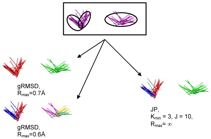
gRMSD clustering vs. JP clustering of ethane molecules. Hydrogens are not shown for clarity. The top image shows three clusters from MCM minimizations, two closely spaced but densely packed clusters and one larger diffuse cluster that spans approximately the same dimensions. gRMSD clustering (left) is too coarse, identifying too few clusters (left-top) or too many (left-bottom) with a minimal change of R_max. JP clustering (right) is able to correctly discriminate between the three clusters. Clusters are identified by color: the purple ethanes in the top image are not clustered. Red, green, blue, purple, yellow, and teal represent different clusters in the lower images. Note that the JP method does not designate the few grey molecules in the lower right image as being part of any cluster.

The example shown in Fig. 2 is by no means unique. In Fig. 3, we present the p53-HDM2 complex. Fig. 3a shows solvent mapping with methanol, as clustered by JP algorithms. This system was chosen because it demonstrates the superiority of JP clustering and also demonstrates the fact that some mapped sites are appropriate but not necessarily complemented by a binding partner. For instance, the purple and orange sites in Fig. 3b represent hydrogen-bonding interactions with backbone carbonyl oxygens (Val93 and Gln72). These are not complemented by p53, but can be successfully used in SBDD [52]. In Fig. 3b, six of the cluster sites directly map to interactions from p53: the black and blue clusters represent the interaction from Glu17, the yellow cluster represents a backbone interaction from Phe19, the pink cluster represents an interaction from Trp23, the green cluster represents a backbone carbonyl interaction from Leu25, and the cyan cluster represents an interaction from the C-terminal carboxylate of the peptide used in the crystal structure. The brown cluster represents an acceptor interaction with the solvent-exposed Lys51 side chain on the edge of the binding cleft. The cluster falls between the Lys51 of HDM2 and the Glu28 of the p53 helix, a position appropriate for a bridging water molecule (no water were resolved in the original crystal structure).

Fig. 3.

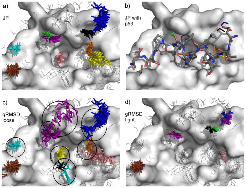
A comparison of JP and gRMSD clustering. Part a) shows the methanol JP clusters for HDM2. In part b), p53 has been overlaid to show its overlap with appropriate clusters. For clarity, only one element from each cluster is shown. Part c) shows the analogous gRMSD clustering at 1.4 Å where we see the typical results of clusters that are much too loose and large (circled); appropriate clusters have been joined together (upper right) and diffuse collections of probes have been marked as either new clusters (bottom center) or parts of other clusters (upper left). An additional problem with gRMSD clustering is that the center of an elongated cluster (e.g. the blue cluster in the upper right of part c) may not be the most energetically favorable location. JP clustering typically alleviates this by separating the cluster into multiple parts. Part d) reducing the gRMSD cutoff to 0.5 Å eliminates this problem, but also eliminates important clusters (circled) and splits some clusters (upper right). The p53/HDM2 system is shown as sticks/surfaces with hydrogens hidden for clarity. Methanol clusters within 3.0 Å of both protein surfaces and containing at least 7 elements are shown in colored sticks. Other methanols are shown in grey lines. For purposes of clarity, some probes outside the binding cleft are not shown, and aliphatic methanol hydrogens are hidden.

Fig. 3c-d demonstrates typical problems encountered with gRMSD clustering (R_max ranging from 0.5-1.4 Å). It was not possible to choose a set of parameters that would reproduce the proper clustering captured by JP. Fig. 2 demonstrates the issues that are encountered when gRMSD parameters are incremented to find parameters that match JP. A total of 7 systems were examined, all of protein-protein recognition events (see Table 2). In 3 of the systems, there were important interactions that were improperly clustered by gRMSD. In 4 systems, results were the same between JP and gRMSD. In some way, these “easy” cases are appropriate because solvent mapping has been successfully used in SBDD [5, 7, 10, 11, 13, 14, 53, 54]. However, to get the correct clustering, each system required individual parameterization. It was necessary to vary the parameters between 0.75-1.25 Å for each individual system. This emphasizes the system-dependant nature of gRMSD clustering; it can often work in a particular case, but parameters are not generalizable. For the other 3 cases, it was not possible to correctly cluster the probes with gRMSD, regardless of our attempts at parameter variation.

Table 2. Comparison of JP and gRMSD clustering across seven protein recognition systems.^a.

Protein System (PDB ID)	# Interactions identified by probes	Properly clustered by JP	Properly clustered by gRMSD	gRMSD cutoff for this system
Barnase-Barstar (1B27) [46]	6	6	4	0.75 Å
CDK6- p16INK4a (1BI7) [49]	5	5	3	0.75 Å
hMms2-hUbc13 (1J7D) [47]	2	2	2	1.25 Å
TRAF6-RANK (1LB5) [48]	2	1	1	1.0 Å
thrombin-BPTI (1BTH) [45]	3	3	3	0.75 Å
CheY-CheA (1EAY) [44]	5	5	5	1.0 Å
HDM2-p53 (1YCR) [43]	6	6	5	0.75 Å

^aFor each system, we recorded the number of hydrogen-bonding interactions found in the natural binding partner that were near clusters of probes (column 2). Column 3 reports how many of those clusters were identified with JP clustering, column 4 the number found with gRMSD clustering, and column 5 gives the optimal gRMSD cutoff required to identify the most clusters appropriate for each system. The cutoff was increased from 0.25 Å to 1.5 Å in steps of 0.25 Å in order to determine this optimal value. When the cutoff is too generous, the reported clusters are too large and diffuse. We have reported the value that was as large as possible without generating this effect.

For an even presentation, we should note that there was one case where JP failed, an interaction with a glutamic acid side chain in TRAF6-RANK. The cluster is a rare case where the probes are slightly too diffuse to be captured by our JP parameters. However, we also note that gRMSD clustering failed in this case. We were not able to find cases where gRMSD clustering performed better than JP clustering.

Applications to structure-based drug design

Our group has a history of success modeling HIV-1 protease [22, 23, 53]. If we re-examine those studies using JP clustering, it generates models that are very comparable to those created by assessing clusters by hand. The structure of the receptor-based pharmacophore models and their performance in identifying known inhibitors over chemically similar decoys are nearly identical (data not shown, but the original models can be found in earlier publications [22]). However, the process is significantly faster using JP clustering. While manually assessing the models can take weeks, the JP clustering takes 15 minutes on a modest 1.0 GHz Intel Pentium II laptop with 256M of memory. Furthermore, it removes the subjective nature of creating models by hand.

To emphasize the improvement that JP offers, we show in Fig. 4 a case that would not be possible to assess manually. The multiple protein structure (MPS) method [13, 23] for SBDD consists of flooding, minimizing, and clustering probes on the surfaces of an ensemble of protein structures. Clusters that are common across the ensemble are identified, and these consensus clusters are used to generate receptor-based pharmacophore models that can be used for lead-generation and SBDD. In developing this model, practitioners of the MPS method must assess clusters for each individual snapshot, choose a representative element from each cluster, and then cluster the representative elements. In Fig 4a, we see the benzene probes from eleven snapshots of an MD simulation [23] (500 probes per snapshot). In Fig 4b, we see the results of applying JP clustering to all 5,500 probes at once (an impossible task by hand): JP clustering results in a model that contains the clusters of the same approximate size and location as the original MPS work. We had to modify the JP parameters in order to cluster such a large system, both increasing the size of the neighbor lists and decreasing the RMSD cutoff. Parameters of (J=250, K_min=3, R_max=0.9 Å) were used for ethane and benzene, and (J=15, K_min=3, R_max=0.75 Å) were used for methanol. In line with the original MPS work, we also required clusters to contain at least one element from the beginning, middle, and end of the simulation. This all-in-one technique has not been broadly applied, and the choice of parameters may not be transferable to other systems.

Fig. 4.

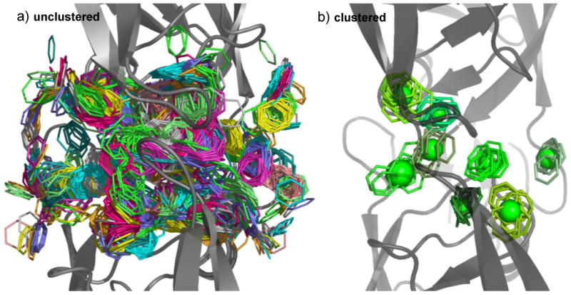
Previously impossible, all-in-one clustering. 5,500 benzene probes are overlaid in part a), 500 each from 11 snapshots of an MD trajectory.[23] All probes from a given snapshot are shown in sticks of the same color. Hydrogens are hidden for clarity, and the protein HIV-1 protease is shown in cartoon. Part b) shows the results of clustering all 5,500 probes at once. Different clusters are shown in different shades of green, and spheres represent the center and RMSD of each cluster.

A final note on the parameters

It is worth recalling the original work of Allen et al. in applying JP clustering to the separation of molecules in physical space [19, 20]. They found great success with JP clustering and provided a preliminary set of clustering criteria for classifying conformational states of six-membered ring compounds. They noted that their parameters were relevant for the particular systems that they had studied, but that further refinement might be necessary as the technique was applied to more diverse systems. Similarly, our parameters have been successful for clustering the particular systems that we have studied, and we feel that they will provide a general starting point for any similar system. Researchers investigating other systems may find it necessary to modify them slightly, but we do not expect great changes from these parameters. Our automated technique has the great advantage that it is orders of magnitude faster than by-hand clustering and less subjective. Thus, when examining a new system, it is a relatively fast and easy task to verify that a correct set of clustering parameters has been chosen. The ranges provided in Table 1 provide a good starting guideline. Users should always take care to verify new parameters by visual inspection of the resulting clusters and through comparisons to hand-generated results. The clustering code that we provide (http://sitemaker.umich.edu/carlsonlab/resources.html) includes scripts that aid in the process of examining and evaluating different parameter sets.

Conclusions

We have developed a fast, easy-to-use set of automated procedures to aid in the mapping of protein surfaces. In particular, we have developed improved procedures for placing small-molecule probes near the site of interest. Once those probes have been minimized to the protein surface, our new technique for clustering the probes shows great success. We have investigated both RMSD-based and JP-based clustering methods, taking the symmetry of the probe molecules into account in all cases. JP-based clustering is more accurate and significantly faster than previous methods like gRMSD and manual processing. Open-source code for flooding and clustering is provided at http://sitemaker.umich.edu/carlsonlab/resources.html.

For validation purposes, we have applied these methods to protein-protein interfaces. We also extended it to our MPS method for SBDD. Our automated techniques produce pharmacophore models that are qualitatively and quantitatively similar to our previous “by-hand” results. These previous results required significant training and time to produce, often taking several weeks for a particular system. The automated methods can perform the same tasks in minutes or hours. Automated methods are also able to cluster thousands of molecules simultaneously, a task that would be impossible by hand.

These methods are robust and may easily be extended to new classes of small molecules. Our automated toolset has been developed as a series of Python scripts and PyMOL plugins and wizards. This makes them easy for other groups to use and extend. Our technique for symmetry-corrected JP clustering could easily be incorporated into other clustering packages such as MCSS, MCSS2PTS, LUDI, or BOSS [5-7, 26, 56]. In addition to these distance-based techniques, interaction-based clustering [14, 15] can also be used in conjunction with JP algorithms, and may be particularly relevant to the study of protein ensembles. The need for better clustering algorithms has been noted in the literature [14, 15].

References

- 1.Vajda S, Guarnieri F. Curr Opin Drug Discov Design. 2006;9:354. [PubMed] [Google Scholar]
- 2.Carr RAE, Congreve M, Murray CW, Rees DC. Drug Discov Today. 2005;10:987. doi: 10.1016/S1359-6446(05)03511-7. [DOI] [PubMed] [Google Scholar]
- 3.Erlanson DA, McDowell RS, O'Brien T. J Med Chem. 2004;47:3463. doi: 10.1021/jm040031v. [DOI] [PubMed] [Google Scholar]
- 4.Rees DC, Congreve M, Murray CW, Carr R. Nat Rev Drug Discov. 2004;3:660. doi: 10.1038/nrd1467. [DOI] [PubMed] [Google Scholar]
- 5.Miranker A, Karplus M. Prot Struct Func Genetics. 1991;11:29. doi: 10.1002/prot.340110104. [DOI] [PubMed] [Google Scholar]
- 6.Schechner M, Dejaegere AP, Stote RH. Int J Quantum Chem. 2004;98:378. [Google Scholar]
- 7.Joseph-McCarthy D, Alvarez JC. Prot Struct Func Bioinfo. 2003;51:189. doi: 10.1002/prot.10296. [DOI] [PubMed] [Google Scholar]
- 8.Hartigan JA, Wong MA. Appl Stat-J Roy St C. 1979;28:100. [Google Scholar]
- 9.Jarvis RA, Patrick EA. IEEE T Comput. 1973;22:1025. [Google Scholar]
- 10.Laurie ATR, Jackson RM. Bioinformatics. 2005;21:1908. doi: 10.1093/bioinformatics/bti315. [DOI] [PubMed] [Google Scholar]
- 11.Caflisch A, Miranker A, Karplus M. J Med Chem. 1993;36:2142. doi: 10.1021/jm00067a013. [DOI] [PubMed] [Google Scholar]
- 12.Evensen E, Joseph-McCarthy D, Weiss GA, Schreiber SL, Karplus M. J Comput-Aided Mol Des. 2007;21:395. doi: 10.1007/s10822-007-9119-x. [DOI] [PubMed] [Google Scholar]
- 13.Carlson HA, Masukawa KM, Rubins K, Bushman FD, Jorgensen WL, Lins RD, Briggs JM, McCammon JA. J Med Chem. 2000;43:2100. doi: 10.1021/jm990322h. [DOI] [PubMed] [Google Scholar]
- 14.Schechner M, Sirockin F, Stote RH, Dejaegere AP. J Med Chem. 2004;47:4373. doi: 10.1021/jm0311184. [DOI] [PubMed] [Google Scholar]
- 15.Sirockin F, Sich C, Improta S, Schaefer M, Saudek V, Froloff N, Karplus M, Dejaegere A. J Am Chem Soc. 2002;124:11073. doi: 10.1021/ja0265658. [DOI] [PubMed] [Google Scholar]
- 16.Arnold JR, Burdick KW, Pegg SC, Toba S, Lamb ML, Kuntz ID. J Chem Inf Comput Sci. 2004;44:2190. doi: 10.1021/ci049814f. [DOI] [PubMed] [Google Scholar]
- 17.Kauffman L, Rousseeuw PJ. Finding groups in data: An introduction to cluster analysis. John Wiley & Sons Inc.; New York: 1990. [Google Scholar]
- 18.Willett P. Similarity and clustering in chemical information systems. John Wiley & Sons Inc.; New York: 1987. [Google Scholar]
- 19.Allen FH, Doyle MJ, Taylor R. Acta Crystallogr B. 1991;47:29. [Google Scholar]
- 20.Allen FH, Doyle MJ, Taylor R. Acta Crystallogr B. 1991;47:41. [Google Scholar]
- 21.Allen FH, Kennard O, Taylor R. Acc Chem Res. 1983;16:146. [Google Scholar]
- 22.Meagher KL, Lerner MG, Carlson HA. J Med Chem. 2006;49:3478. doi: 10.1021/jm050755m. [DOI] [PubMed] [Google Scholar]
- 23.Meagher KL, Carlson HA. J Am Chem Soc. 2004;126:13276. doi: 10.1021/ja0469378. [DOI] [PubMed] [Google Scholar]
- 24.Lerner MG, Bowman AL, Carlson HA. J Chem Inf Model. 2007;47:2358. doi: 10.1021/ci700167n. [DOI] [PubMed] [Google Scholar]
- 25.Bowman AL, Lerner MG, Carlson HA. J Am Chem Soc. 2007;129:3634. doi: 10.1021/ja068256d. [DOI] [PubMed] [Google Scholar]
- 26.Jorgensen WL. BOSS V4.2. Yale University; New Haven, CT: 2000. [Google Scholar]
- 27.Jones S, Thornton JM. Proc Natl Acad Sci USA. 1996;93:13. [Google Scholar]
- 28.Arkin MR, Wells JA. Nat Rev Drug Discov. 2004;3:301. doi: 10.1038/nrd1343. [DOI] [PubMed] [Google Scholar]
- 29.Wells JA, McClendon CL. Nature. 2007;450:1001. doi: 10.1038/nature06526. [DOI] [PubMed] [Google Scholar]
- 30.Keskin O, Tsai CJ, Wolfson H, Nussinov R. Protein Sci. 2004;13:1043. doi: 10.1110/ps.03484604. [DOI] [PMC free article] [PubMed] [Google Scholar]
- 31.Ofran Y, Rost B. J Mol Biol. 2003;325:377. doi: 10.1016/s0022-2836(02)01223-8. [DOI] [PubMed] [Google Scholar]
- 32.Salwinski L, Miller CS, Smith AJ, Pettit FK, Bowie JU, Eisenberg D. Nucleic Acids Res. 2004;32:D449. doi: 10.1093/nar/gkh086. [DOI] [PMC free article] [PubMed] [Google Scholar]
- 33.Xenarios I, Salwinski L, Duan XJ, Higney P, Kim SM, Eisenberg D. Nucleic Acids Res. 2002;30:303. doi: 10.1093/nar/30.1.303. [DOI] [PMC free article] [PubMed] [Google Scholar]
- 34.Larsen TA, Olson AJ, Goodsell DS. Structure. 1998;6:421. doi: 10.1016/s0969-2126(98)00044-6. [DOI] [PubMed] [Google Scholar]
- 35.Reichmann D, Rahat O, Albeck S, Meged R, Dym O, Schreiber G. Proc Natl Acad Sci USA. 2005;102:57. doi: 10.1073/pnas.0407280102. [DOI] [PMC free article] [PubMed] [Google Scholar]
- 36.DeLano WL. Curr Opin Struct Biol. 2002;12:14. doi: 10.1016/s0959-440x(02)00283-x. [DOI] [PubMed] [Google Scholar]
- 37.Janin J. Protein Sci. 2005;14:278. doi: 10.1110/ps.041081905. [DOI] [PMC free article] [PubMed] [Google Scholar]
- 38.Ehrlich LP, Nilges M, Wade RC. Prot Struct Func Bioinfo. 2005;58:126. doi: 10.1002/prot.20272. [DOI] [PubMed] [Google Scholar]
- 39.Berman HM, Westbrook J, Feng Z, Gilliland G, Bhat TN, Weissig H, Shindyalov IN, Bourne PE. Nucleic Acids Res. 2000;28:235. doi: 10.1093/nar/28.1.235. [DOI] [PMC free article] [PubMed] [Google Scholar]
- 40.Lovell SC, Davis IW, Arendall WB, III, de Bakker PIW, Word JM, Prisant MG, Richardson JS, Richardson DC. Prot Struct Func Genetics. 2003;50:437. doi: 10.1002/prot.10286. [DOI] [PubMed] [Google Scholar]
- 41.DeLano WL. The PyMOL Molecular Graphics System. Palo Alto, CA, USA: 2002. [Google Scholar]
- 42.Case DA, Darden TA, Cheatham TE, III, Simmerling CL, Wang J, Duke RE, Luo R, Merz KM, Wang B, Pearlman DA, Crowley M, Brozell S, Tsui V, Gohlke H, Mongan J, Hornak V, Cui G, Beroza P, Schafmeister C, Caldwell JW, Ross WS, Kollman PA. AMBER 8. University of California, San Francisco; San Francisco, CA: 2004. [Google Scholar]
- 43.Kussie PH, Gorina S, Marechal V, Elenbaas B, Moreau J, Levine AJ, Pavletich NP. Science. 1996;274:948. doi: 10.1126/science.274.5289.948. [DOI] [PubMed] [Google Scholar]
- 44.McEvoy MM, Hausrath AC, Randolph GB, Remington SJ, Dahlquist FW. Proc Natl Acad Sci USA. 1998;95:7333. doi: 10.1073/pnas.95.13.7333. [DOI] [PMC free article] [PubMed] [Google Scholar]
- 45.van de Locht A, Bode W, Huber R, Bonniec BFL, Stone SR, Esmon CT, Stubbs MT. EMBO J. 1997;16:2977. doi: 10.1093/emboj/16.11.2977. [DOI] [PMC free article] [PubMed] [Google Scholar]
- 46.Buckle AM, Schreiber G, Fersht AR. Biochemistry. 1994;33:8878. doi: 10.1021/bi00196a004. [DOI] [PubMed] [Google Scholar]
- 47.Moraes TF, Edwards RA, McKenna S, Pastushok L, Xiao W, Glover JNM, Ellison MJ. Nat Struct Mol Biol. 2001;8:669. doi: 10.1038/90373. [DOI] [PubMed] [Google Scholar]
- 48.Ye H, Arron JR, Lamothe B, Cirilli M, Kobayashi T, Shevde NK, Segal D, Dzivenu OK, Vologodskaia M, Yim M, Du K, Singh S, Pike JW, Darnay BG, Choi Y, Wu H. Nature. 2002;418:443. doi: 10.1038/nature00888. [DOI] [PubMed] [Google Scholar]
- 49.Russo AA, Tong L, Lee JO, Jeffrey PD, Pavletich NP. Nature. 1998;395:237. doi: 10.1038/26155. [DOI] [PubMed] [Google Scholar]
- 50.Crowley PB, Golovin A. Prot Struct Func Bioinfo. 2005;59:231. doi: 10.1002/prot.20417. [DOI] [PubMed] [Google Scholar]
- 51.Jorgensen WL, Maxwell DS, Tirado-Rives J. J Am Chem Soc. 1996;118:11225. [Google Scholar]
- 52.Bowman AL, Nikolovska-Coleska Z, Zhong H, Wang S, Carlson HA. J Am Chem Soc. 2007;129:12809. doi: 10.1021/ja073687x. [DOI] [PubMed] [Google Scholar]
- 53.Damm KL, Carlson HA. J Am Chem Soc. 2007;129:8225. doi: 10.1021/ja0709728. [DOI] [PubMed] [Google Scholar]
- 54.Damm KL, Ung PMU, Quintero JJ, Gestwicki JE, Carlson HA. Biopolymers. 2008;89:643. doi: 10.1002/bip.20993. [DOI] [PMC free article] [PubMed] [Google Scholar]
- 55.Duda RO, Hart PE, Stork DG. Pattern classification. Wiley-Interscience; New York: 2000. [Google Scholar]
- 56.Böhm HJ. J Comput-Aided Mol Des. 1992;6:61. doi: 10.1007/BF00124387. [DOI] [PubMed] [Google Scholar]
Associated Data
This section collects any data citations, data availability statements, or supplementary materials included in this article.