Haseman Elston Regression in Ascertained Samples: Importance of Dependent Variable and Mean Correction Factor Selection

Abstract

Objective

One of the first tools for performing linkage analysis, Haseman-Elston regression (HE), has been successfully used to identify linkages to several disease traits. A recent explosion in extensions of HE leaves one faced with the task of choosing a flavor of HE best suited for a given situation. This paper puts this dilemma into perspective and proposes a modification to HE for highly ascertained samples (BLUP-PM).

Methods

Using data simulated for a range of models, we evaluated type I error and power of several dependent variables in HE, including the novel BLUP-PM.

Results

When analyzing a continuous trait, even in highly ascertained samples, type I error is stable and approximately nominal across dependent variables. When analyzing binary traits in highly ascertained samples, type I error is elevated and unstable for all except BLUP-PM. Regardless of trait type, the optimally weighted HE regression and BLUP-PM have the greatest power.

Conclusions

Ascertained samples do not always reflect the population from which they are drawn and therefore choice of dependent variable in HE becomes increasingly important. Our results do not reveal a single, universal choice, but offer criteria by which to choose and demonstrate BLUP-PM performs well in most situations.

Introduction

Efforts to identify genes predisposing to or protecting against common complex disease have been at the forefront of epidemiological research over the last 30 years; linkage studies in particular. Unfortunately, however, these studies are often riddled with difficult decisions, from choosing the most efficient ascertainment scheme and correct phenotype measure, to the most appropriate and powerful statistical technique. One tool that has proven to be both powerful and robust for the mapping of trait loci is Haseman-Elston regression (HE). This robust test to detect linkage between a putative disease locus and a marker locus was first proposed in 1972 [1] and has since been revised [2] and extended several times [3,4,5,6,7,8,9,10].

Consider the situation where we have n sibling pairs, which may or may not be independent. For the j-th sibling pair let their trait values be (x_1j, x_2j), for either a continuous or a dichotomous trait. The original HE [1] regresses the squared trait difference, (x_1j – x_2j)², on the average identical by descent (IBD) allele sharing for the j-th pair π‸_j. Replacing the squared trait difference with the mean corrected cross product:

$$\frac{1}{4}\left[{\left(\left(x_{1j}-\mu \right)+\left(x_{2j}-\mu \right)\right)}^2-{\left(\left(x_{1j}-\mu \right)-\left(x_{2j}-\mu \right)\right)}^2\right],$$ (1)

leads to an increase in the power of HE in some situations [2], largely depending on the residual sibling correlation [5]. Since the original HE can be more powerful than the cross product in some situations, the following dependent variable:

$$\frac{1}{4}\left[w_j{\left(\left(x_{1j}-\mu \right)+\left(x_{2j}-\mu \right)\right)}^2-\left(1-w_j\right){\left(\left(x_{1j}-\mu \right)-\left(x_{2j}-\mu \right)\right)}^2\right],$$ (2)

which is a weighted sum of the mean corrected sum and difference, with optimally chosen weights was proposed [6].

In a further extension, it was shown that when using the cross product, replacing μ with the Best Linear Unbiased Predictor (BLUP) of μ_j, the mean of the j-th sibship (assuming a random mean model), leads to better results than the optimally weighted cross product [11]. The authors also showed that such a dependent variable did not require adjustment for dependence between sibling pairs in a sibship. In particular, the BLUP of μ_j is given by:

$${\overline{\mu }}_j=w_j^{*}{\overline{X}}_j+\left(1-w_j^{*}\right)\stackrel{‸}{\mu },$$ (3)

where the weights, w*_j, are determined by the between and within sibship variances and the size of the sibship. The term X–_j is the mean of the j-th sibship and $\stackrel{‸}{\mu }$, is an estimate of the overall, or population, mean, taken to be the sample mean. Often, however, a sample is ascertained for individuals with extreme values of a trait or in the case of a binary trait, presence of the phenotype of interest, rendering the sample mean a poor estimate of the population mean. In this study, we propose yet another revision to HE for highly ascertained samples and evaluate both type I error and power for many of the dependent variable options for HE as available in the software SIBPAL, implemented in the program package S.A.G.E.. We further offer a guide by which to determine the dependent variable that is most suitable given either continuous or binary phenotypes and various ascertainment schemes and modes of inheritance.

A binary trait is a special case of a quantitative trait, and hence HE can be applied without any modifications [12]. The only requirement of this application of HE is that the sample has discordant as well as concordant sibling pairs. This requirement is often satisfied simply because, when multiplex families are ascertained, unaffected siblings are collected and genotyped to increase information to infer IBD sharing. HE has been shown to have correct type I error and good power with unaffected siblings providing linkage information as shown by both our own results and Davis et al. [13]. Further, the affected/discordant-sib-pair design guards against possible biases due to Mendelian transmission distortions [14] and biased estimation of multi-point IBD sharing probabilities due to marker to marker linkage disequilibrium [15]. Finally, unlike some likelihood based methods, HE, as implemented in S.A.G.E., correctly handles dependencies in large sibships using Generalized Estimating Equations.

Methods

Simulation

To explore the different dependent variables available in HE, we simulated quantitative traits, both continuous and binary, to reflect realistic data for common, complex diseases. We further employed ascertainment schemes most common to genetic epidemiological studies today.

Continuous Traits

For the continuous traits we simulated nuclear families with three siblings each. The sample size was taken to be 250 families, leading to 750 sibling pairs when the families were ascertained using the 70th percentile of the population trait value. When the 90th percentile was used, we took a sample size of 100 pedigrees, leading to 300 sibling pairs, this difference in sample sizes was to demonstrate power at levels where differences were appreciable and results distinguishable (i.e. analyses of 250 families ascertained at the 90% level would yield close to 100% power for all models).

Two basic models, ‘Strong’ and ‘Weak’ (table 1) were simulated with total variance (V_T) of 20. Both had equal additive and genetic variance (V_A and V_G, respectively). Strong had a large residual variance due to environment (V_C) and a strong residual sibling correlation (r), while Weak had a lesser residual environmental variance and more than 2-fold lesser r. Both models had heritabilities less than 20%. To model often used ascertainment schemes (table 1), a family was ascertained if at least k siblings, where k = 1, 2, had trait values equal or greater than the 70th and 90th percentile of the population trait values. SS is used to designate single simplex ascertainment, in which a family was ascertained if one member met criteria (i.e., k = 1), and SM designates single, multiplex ascertainment in which at least 2 members of the family met the criteria for ascertainment (i.e., k = 2).

Table 1.

Parameter values used to simulate a continuous trait

Familial correlation	VA = VG	VC	VT	r	Herita- bility, %	Ascertainment
						cut-off, %	number of sibs attaining cut-off
Strong	3	5	20	0.325	15	70, 90	1, 2
Weak	2	2	20	0.15	10	70, 90	1, 2

As mentioned, the power of the various dependent variables in HE to detect linkage to a quantitative trait locus is closely related to the sib-sib correlation. In particular, the squared difference is a more powerful dependent trait than the cross product when the sib-sib correlation is greater than (2 – √3) = 0.268 (proof shown in the Appendix). However, because of possible ascertainment, the sib-sib correlation in selected samples is not the same as the true population sib-sib correlation. Table 2 gives the estimated sib-sib correlation in a large ascertained population for various ascertainment schemes. These values were estimated using FCOR [16], from 2,500 simulated families with three siblings each and denoted trait model and ascertainment scheme.

Table 2.

Estimates and standard errors of sib-sib correlation in 2,500 families with three siblings

Familial correlation	Ascertainment	Cut-off %	Estimated sib-sib correlation	Standard error
Strong	none		0.3271	0.0074
	SM	70	–0.0442	0.0110
		90	–0.1633	0.0090
	SS	70	0.0322	0.0119
		90	–0.0886	0.0103
Weak	none		0.1486	0.0074
	SM	70	–0.1800	0.0087
		90	–0.2529	0.0071
	SS	70	–0.0864	0.0104
		90	–0.1928	0.0085

Binary Traits

For the binary traits, we simulated 400 families each with four siblings, of whom two were affected and two were unaffected, resulting in families with one pair of affected siblings, one pair of unaffected siblings and four discordant sibling pairs.

Two disease models were simulated, both with a prevalence of approximately 4%, a phenocopy rate of 4% and heritability of 1.8% (when all families are linked to the disease locus). The recessive model (Rec), and the dominant model with a low penetrance of disease allele (Dom) had underlying disease locus genotype (f_DD, f_Dd, f_dd) frequencies corresponding to an 8 and 4% sporadic rate, respectively. In addition we simulated varying degrees of heterogeneity in the population, that is, a portion of the sample is simulated using the disease model and the rest are assigned null chromosomes (table 3).

Table 3.

Parameter values used to simulate a binary trait

Model	P(D)	fDD	fDd	fdd	Proportion not linked	Herita- bility	Preva- lence
Rec	0.04	0.70	0.04	0.04	0.0 0.5 0.75	1.8%	4.1%
Dom	0.01	0.24	0.24	0.04	0.0 0.5 0.75	1.8%	4.4%

Analysis Methods

As mentioned, there are several options for the dependent variable to be used in HE. The options to be evaluated as a part of study include: the difference in the two siblings’ trait values [1], referred to as ‘Diff’; the mean-corrected cross product of the two siblings’ trait values [2], referred to as ‘Prod’; the weighted combination of the ‘Diff’ and mean-corrected sum (Sum) of the two siblings’ trait values assuming difference and sum are independent [16] referred to as ‘W2’; the weighted combination of the Diff and Sum of the two siblings’ trait values further allowing for the correlation between sibling pairs within a sibship [16], referred to as ‘W3’; the weighted combination of the Diff and Sum of the two siblings’ trait values allowing for the correlation between sib-pairs within a sibship as well as the correlation of the Diff and Sum [6], referred to as ‘W4’. All of these, with the exclusion of ‘Diff’, require specification of a ‘mean’ value, μ, for the trait. In a random sample from the population, the sample mean provides a reasonable estimate of the population mean μ. However, samples are often enriched with extreme values of the trait of interest to increase the possibility of identifying linkage. In such a situation the sample mean is no longer a good estimate of the population mean and the choice of μ becomes even more important. It is our hypothesis that, while the BLUP of μ_j (Equation 3), in which μ‸ is taken to be the sample mean (from here forward referred to as BLUP-SM), performs quite well in most situations. However, in the presence of strong ascertainment, a dependent variable in which the estimate of the population mean is used in place of the sample mean for μ‸ (referred to now as BLUP-PM) will perform better, assuming, of course, that the population mean is well estimated from independent epidemiologic studies. It is important to note that while this study focuses on the selection of the mean, HE, as with other regression based methods, does require estimation of the variance. This is done, using either Generalized Least Square regression or, when accounting for the dependence of observations, Generalized Estimating Equations.

To compare the type I error of the various dependent variables in HE (table 4), we analyzed, for the continuous and binary traits, 2,000 and 5,000 replicates, respectively, simulated under the null hypothesis of no linkage. To compare power for both the continuous and binary traits, we analyzed 1,000 replicates simulated under the alternate hypothesis of linkage. SIBPAL, a subroutine of the program package S.A.G.E. (v5.2) and a script in R [17] were used for all analyses.

Table 4.

Dependent variables compared in this study

Dependent variable name	Definition
Diff∗	–1/2 × squared trait difference
Prod∗	Mean-corrected cross-product, m equal to either the sample mean or a pre-specified value
W2∗	Weighted combination of squared trait difference and squared mean-corrected trait sum. Weights are chosen pro- portional to the inverses of the residual variances of the squared differences and sums.
W3∗	Weighted combination of squared trait difference and squared mean-corrected trait sum, as W2 but further adjusted for the possible non-independence of sib-pairs.
W4∗	Weighted combination of squared trait difference and squared mean-corrected trait sum, as W3 but further adjusted for the non-independence of sib-pairs and the non-independence of squared trait sums and differences.
BLUP-SM∗	Mean-corrected cross-product, m equal to the BLUP of the sibship mean, assuming a random sibship mean model; sample mean used to represent the overall mean
BLUP-PM	Mean-corrected cross-product, m equal to the BLUP of the sibship mean, assuming a random sibship mean model; population mean used to represent the overall mean

^∗Denotes features available in SIBPAL, a subroutine of the program package S.A.G.E. Details of each of these options can be found in the S.A.G.E., Version 5.3 User Manual pages 235–244.

Results

Continuous Traits

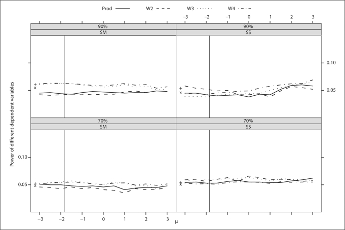
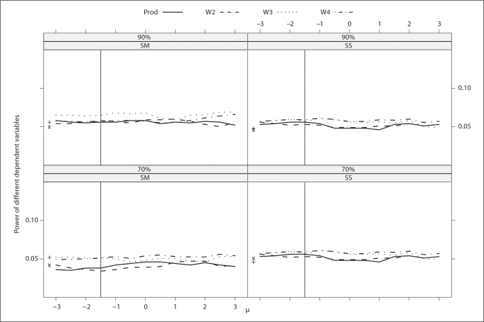
The type I error rates are comparable and close to the nominal level across dependent variables, strength of familial correlation, ascertainment scheme, level of ascertainment (table 5), and values of μ(fig. 1 and 2).

Table 5.

Type I errors of using different dependent variables for a continuous trait, Diff, Prod, W2, W3 and W4, with the sample mean, BLUP-SM, and BLUP-PM

Familial correlation	Ascertainment	Cut-off %	Dependent variable
			Diff	Prod	W2	W3	W4	BLUP-SM	BLUP-PM
Strong	SM	70	0.053	0.044	0.045	0.051	0.051	0.044	0.049
		90	0.061	0.051	0.052	0.061	0.061	0.051	0.055
	SS	70	0.054	0.052	0.054	0.055	0.055	0.052	0.051
		90	0.054	0.056	0.055	0.060	0.060	0.056	0.046
Weak	SM	70	0.052	0.046	0.044	0.054	0.054	0.046	0.042
		90	0.056	0.055	0.054	0.057	0.057	0.055	0.050
	SS	70	0.046	0.048	0.050	0.058	0.058	0.048	0.051
		90	0.048	0.048	0.049	0.052	0.052	0.048	0.046

Fig. 1.

Trait with strong familial correlation. Type I errors of different dependent variables for a continuous trait with different levels and schemes of ascertainment. The abscissa of the vertical line denotes a known population mean of the trait. The ordinates of ‘x’ and ‘+’ denote the type I error of BLUP-PM and Diff, respectively.

Fig. 2.

Trait with weak familial correlation. Type I errors of different dependent variables for a continuous trait with different levels and schemes of ascertainment. The abscissa of the vertical line denotes a known population mean of the trait. The ordinates of ‘x’ and ‘+’ denote the type I error of BLUP-PM and Diff, respectively.

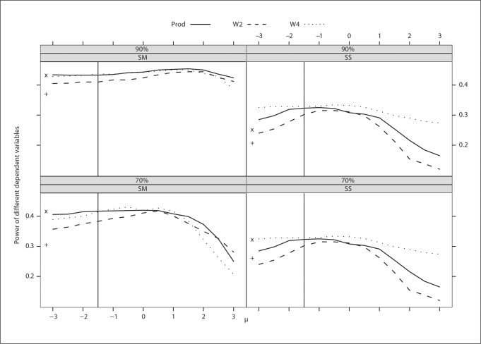
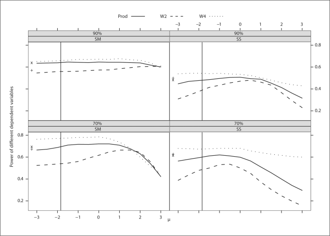
Power for the dependent variables, depending on the strength of the residual familial correlation and the sampling scheme varies from 0.207 to 0.696 (table 6), when using the sample mean in conjunction with the dependent variables Prod, W2, W3 and W4. The power of these same dependent variables used in conjunction with the population mean can be read from the figures 3 and 4 (indicated by the vertical lines). The power of BLUP-PM, on the other hand does not correspond to any value of the abscissa and hence included only in the tables. As explained earlier, these values were kept purposefully low. Because we were interested in seeing differences in the various options, we maintained a power level that would most accentuate these differences. BLUP-PM performs well in a number of the situations, with the biggest gains for the SM ascertainment. W4 performs well when the sample mean is close to the population mean, which is true for SS ascertainment with 70% cut-off, and Diff performs well (best in one situation) for a trait with strong familial correlation but poorly for a trait with low familial correlation. W3 and W4 perform similarly across models when using the sample mean while BLUP-PM performs better than BLUP-SM in all models, the difference being most pronounced when the population and sample means differ substantially. Note that the BLUP- SM and BLUP-PM are only used in conjunction with ‘Prod’. This is because using BLUP leads to independence of the cross-product between sibling pairs and such independence renders the corrections involved in W2, W3, and W4 unnecessary.

Table 6.

Power of using different dependent variables for a continuous trait, Diff, Prod, W2, W3 and W4, with the sample mean, BLUP-SM, and BLUP-PM

Familial correlation	Ascertainment	Cut-off %	Dependent variable
			Diff	Prod	W2	W3	W4	BLUP-SM	BLUP-PM
Strong	SM	70	0.672	0.645	0.654	0.619	0.619	0.647	0.696
		90	0.571	0.520	0.574	0.400	0.400	0.520	0.641
	SS	70	0.629	0.591	0.497	0.681	0.681	0.613	0.617
		90	0.501	0.448	0.426	0.473	0.473	0.448	0.484
Weak	SM	70	0.305	0.373	0.353	0.332	0.332	0.373	0.417
		90	0.370	0.382	0.380	0.237	0.237	0.382	0.433
	SS	70	0.261	0.305	0.309	0.329	0.329	0.305	0.323
		90	0.207	0.225	0.222	0.235	0.235	0.225	0.252

Fig. 3.

Trait with strong familial correlation. Power of different dependent variables for a continuous trait with different levels and schemes of ascertainment. The power of W3 was not plotted because it was the same as that of W4. The abscissa of the vertical line denotes a known population mean of the trait. The ordinates of ‘x’ and ‘+’ denote the power of BLUP-PM and Diff, respectively.

Fig. 4.

Trait with weak familial correlation. Power of different dependent variables for a continuous trait with different levels and schemes of ascertainment. The power of W3 was not plotted because it was the same as that of W4. The abscissa of the vertical line denotes a known population mean of the trait. The ordinates of ‘x’ and ‘+’ denote the power of BLUP-PM and Diff, respectively.

Over a range of μ values, the powers of W3 and W4 are exactly the same regardless of the strength of the familial correlation and hence, the power curve for W3 is not plotted in figures 3 and 4. Note that W4 performs well over the entire range of μand has consistently more power than Prod. BLUP-PM performs reasonably well for most situations but, because it is bounded by the power curve of Prod, is always less powerful than W4. Using W4 with the population mean (represented by a solid vertical line) performs well for all situations (fig. 3 and 4).

Binary Traits

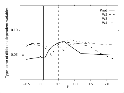
Across models, the type I error rate is slightly elevated (∼0.07) and quite unstable, except BLUP-PM, which has a type I error rate that is close to the nominal (fig. 5).

Fig. 5.

Type I error of different dependent variables for a binary trait. The solid vertical line is a known population mean and the dashed vertical line is the sample mean, as calculated from the observed data. The ordinates of ‘x’ and ‘+’ denote the power of BLUP-PM and Diff, respectively.

For a binary trait, the power does not vary greatly by dependent variables: Prod, W2, W3 and W4 with the sample mean, and Diff (table 7). Using BLUP-PM leads to improved power, except for a recessive disease with high heterogeneity. As expected the power decreases when a smaller percent of families are linked to the locus (i.e. heterogeneity). BLUP-SM is ignored in the table because it has the same power as Prod with sample mean.

Table 7.

Power of using different dependent variables for a binary trait, Diff, Prod, W2, W3 and W4, with the sample mean, and BLUP-PM

Model	Proportion not linked	Dependent variable
		Diff	Prod	W2	W3	W4	BLUP-prod
Recessive	0	0.555	0.555	0.555	0.555	0.556	0.624
	0.5	0.274	0.274	0.274	0.274	0.274	0.289
	0.75	0.147	0.147	0.147	0.147	0.149	0.121
Dominant	0	0.519	0.519	0.519	0.519	0.521	0.662
	0.5	0.226	0.226	0.226	0.226	0.226	0.291
	0.75	0.130	0.130	0.130	0.130	0.130	0.133

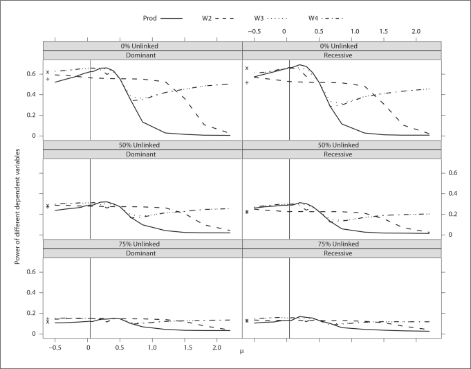
Across values of μ, the power of the different dependent variables is quite variable, but highest around the population mean value or prevalence (0.04, denoted by the solid vertical line in fig. 6). Using W4 with the population mean provides close to optimal power. However, as shown in figure 5, the type I error of W4 is elevated. As a result, it might be better to use BLUP-PM, which has the correct type I error and close to optimal power for all dominant models and the recessive model with no heterogeneity.

Fig. 6.

Power of different dependent variables over a range of μ values for a binary trait with different modes of inheritance and levels of heterogeneity. The solid vertical line denotes the population mean. The ordinates of ‘x’ and ‘+’ denote the power of BLUPPM and Diff, respectively.

Discussion

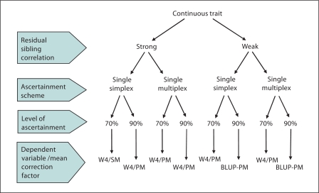
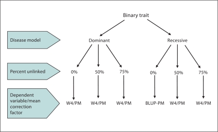
As shown in table 2, the properties of an ascertained sample do not always reflect that of the population from which it is drawn. For this reason, and others, careful attention should be given in choosing an analysis method for an ascertained sample, to both minimize false positives and maximize power. It was the aim of this study to (1) offer a slight modification of the HE for highly ascertained samples, (2) report the type I error and power of various dependent variables for HE in light of this ascertainment, and (3) provide users of HE a guide by which to choose a dependent variable most suited for their particular study and trait of interest. As can be seen in figures 7 and 8, no one method or choice of mean correction factor is always superior. However, in the case of a continuous trait, for the models we examined, W3 and W4 perform consistently better than the others. For a binary trait, the BLUP-PM is consistently better, but the power of all models is highly dependent on the choice of the mean correction factor. Certainly, the more one knows about the trait of interest the more informed the decision. However, we are not always so enlightened and must therefore choose a method that, while it may not be the most powerful in a particular situation, is consistently powerful across models, with correct type I error. In linkage studies, particularly now that we have the capability of generating data every few kb, it is important to protect against a large number of false positives while at the same time preserving as much power as possible. In this study, we provide users of the HE yet another option in doing this. We offer a recommendation of statistical technique, given a variety of study designs, underlying genetic model, and amount of information.

Fig. 7.

Choice of dependent variable and mean correction factor given various scenarios for a continuous trait.

Fig. 8.

Choice of dependent variable and mean correction factor given various scenarios for a binary trait.

Appendix

For a set of independent sibling pairs, let x_ij be the trait value of sib i in pair j; μ be the overall mean; g_ij be the effect of a quantitative trait locus; p_ij be a polygenic effect; c_jbe a common sibship environmental effect; and e_ij be a sib specific random effect. A general model describing the trait value is given by

$$x_{ij}=\mu +g_{ij}+p_{ij}+c_j+e_{ij}$$

Assume that polygenic, common-environmental and random effects are independently and identically distributed as N(0, σ²_p), N(0,σ²_c) and N(0,σ²_e), respectively. Then the variance of the trait value is given by

$$V={\sigma }_g^2+{\sigma }_p^2+{\sigma }_c^2+{\sigma }_e^2,$$

and the covariance between the trait values of the two sibs is

$$C=\frac{k}{2}{\sigma }_g^2+\frac{{\sigma }_p^2}{2}+{\sigma }_c^2,$$

where k is the number of alleles shared IBD. Also, let r = C/V be the correlation between two sibling trait values and define D = −1/2(x_1j – x_2j)² and S = 1/2(x_1j + x_2j − 2μ)².

Let R² be the proportion of the variance of the dependent variable explained by $\stackrel{‸}{\pi }$. Then, Wang & Elston [11] show that R²_o and R²_CP, the R² values for the original HE and cross product, respectively, are given by

$$R_0^2=\frac{{\beta }_0^{2}V\left(\stackrel{‸}{\pi }\right)}{V\left(-2D\right)}=\frac{{\sigma }_G^{2}V\left(\stackrel{‸}{\pi }\right)}{2{\left(1-r\right)}^2}$$

and

$$R_{CP}^2=\frac{{\beta }_{CP}^{2}V\left(\stackrel{‸}{\pi }\right)}{V\left(\frac{1}{2}D+\frac{1}{2}S\right)}=\frac{{\sigma }_G^{2}V\left(\stackrel{‸}{\pi }\right)}{\frac{1}{2}\left[{\left(1+r\right)}^2+{\left(1-r\right)}^2\right]},$$

and

$$\begin{array}{c}{R}_0^2>R_{CP}^2\\ \iff 1+r^2>2{\left(1-r\right)}^2\\ \iff r>2-\sqrt{3}=\mathrm{0.268.}\end{array}$$

The above implies that, when the sib-sib correlation is greater than 0.268, the Diff has more power than the Prod.

References

- 1.Haseman JK, Elston RC. The investigation of linkage between a quantitative trait and a marker locus. Behav Genet. 1972;2:3–19. doi: 10.1007/BF01066731. [DOI] [PubMed] [Google Scholar]
- 2.Elston RC, Buxbaum S, Jacobs KB, Olson JM. Haseman and Elston revisited. Genet Epidemiol. 2000;19:1–17. doi: 10.1002/1098-2272(200007)19:1<1::AID-GEPI1>3.0.CO;2-E. [DOI] [PubMed] [Google Scholar]
- 3.Etzel CJ, Shete S, Beasley TM, Fernandez JR, Allison DB, Amos CI. Effect of Box-Cox transformation on power of Haseman-Elston and maximum-likelihood variance components tests to detect quantitative trait loci. Hum Hered. 2003;55:108–116. doi: 10.1159/000072315. [DOI] [PubMed] [Google Scholar]
- 4.Forrest WF. Weighting improves the ‘new Haseman-Elston’ method. Hum Hered. 2001;52:47–54. doi: 10.1159/000053353. [DOI] [PubMed] [Google Scholar]
- 5.Palmer LJ, Jacobs KB, Elston RC. Haseman and Elston revisited: the effects of ascertainment and residual familial correlations on power to detect linkage. Genet Epidemiol. 2000;19:456–460. doi: 10.1002/1098-2272(200012)19:4<456::AID-GEPI15>3.0.CO;2-N. [DOI] [PubMed] [Google Scholar]
- 6.Shete S, Jacobs KB, Elston RC. Adding further power to the Haseman and Elston method for detecting linkage in larger sibships: weighting sums and differences. Hum Hered. 2003;55:79–85. doi: 10.1159/000072312. [DOI] [PubMed] [Google Scholar]
- 7.Single RM, Finch SJ. Gain in efficiency from using generalized least squares in the Haseman-Elston test. Genet Epidemiol. 1995;12:889–894. doi: 10.1002/gepi.1370120660. [DOI] [PubMed] [Google Scholar]
- 8.Wiener H, Elston RC, Tiwari HK. X-linked extension of the revised Haseman-Elston algorithm for linkage analysis in sib pairs. Hum Hered. 2003;55:97–107. doi: 10.1159/000072314. [DOI] [PubMed] [Google Scholar]
- 9.Wright FA. Information perspectives of the Haseman-Elston method. Hum Hered. 2003;55:132–142. doi: 10.1159/000072318. [DOI] [PubMed] [Google Scholar]
- 10.Xu X, Weiss S, Xu X, Wei LJ. A unified Haseman-Elston method for testing linkage with quantitative traits. Am J Hum Genet. 2000;67:1025–1028. doi: 10.1086/303081. [DOI] [PMC free article] [PubMed] [Google Scholar]
- 11.Wang T, Elston RC. A modified revisited Haseman-Elston method to further improve power. Hum Hered. 2004;57:109–116. doi: 10.1159/000077548. [DOI] [PubMed] [Google Scholar]
- 12.Elston RC, Song D, Iyengar SK. Mathematical assumptions versus biological reality: myths in affected sib pair linkage analysis. Am J Hum Genet. 2005;76:152–156. doi: 10.1086/426872. [DOI] [PMC free article] [PubMed] [Google Scholar]
- 13.Davis S, Weeks DE. Comparison of nonparametric statistics for detection of linkage in nuclear families: Single-marker evaluation. Am J Hum Genet. 1997;61:1431–1444. doi: 10.1086/301635. [DOI] [PMC free article] [PubMed] [Google Scholar]
- 14.Lemire M, Roslin NM, Laprise C, Hudson TJ, Morgan K. Transmission-ratio distortion and allele sharing in affected sib pairs: A new linkage statistic with reduced bias, with application to chromosome 6q25.3. Am J Hum Genet. 2004;75:571–586. doi: 10.1086/424528. [DOI] [PMC free article] [PubMed] [Google Scholar]
- 15.Xing C, Sinha R, Xing G, Lu Q, Elston RC. The affected-/discordant-sib-pair design can guarantee validity of multipoint model-free linkage analysis of incomplete pedigrees when there is marker-marker disequilibrium. Am J Hum Genet. 2006;79:396–401. doi: 10.1086/506331. [DOI] [PMC free article] [PubMed] [Google Scholar]
- 16.Statistical Analysis for Genetic Epidemiology (S.A.G.E.). Version 5.3, 2006.
- 17.R Development Team Core: R: A language and environment for statistical computing. 2005.