FM Reconstruction of Non-Uniformly Sampled Protein NMR Data at Higher Dimensions and Optimization by Distillation

Abstract

Non-uniform sampling (NUS) enables recording of multidimensional NMR data at resolutions matching the resolving power of modern instruments without using excessive measuring time. However, in order to obtain satisfying results, efficient reconstruction methods are needed. Here we describe an optimized version of the Forward Maximum entropy (FM) reconstruction method, which can reconstruct up to three indirect dimensions. For complex datasets, such as NOESY spectra, the performance of the procedure is enhanced by a distillation procedure that reduces artifacts stemming from intense peaks.

Introduction

Multi-dimensional NMR spectra are traditionally recorded by uniformly sampling all complex points through each indirect dimension. To reach the maximal resolution attainable by modern NMR spectrometers would, however, require unreasonably long measurement times. Thus, this spectral resolution is typically sacrificed by sampling only to relatively short evolution times thereby under exploiting the advantages of expensive high-field spectrometers. For example, a typical 3D HNCO experiment records only 50 and 25 points in the indirect nitrogen and carbon dimensions, respectively, which is far from the optimal range (Rovnyak, Hoch et al., 2004). In fact, with identical measurement times (identical number of increments) and spectral widths in ppm, lower spectral resolution is obtained at high field because the shorter dwell times lead to shorter maximum evolution times. Obviously the losses in resolution limit the precision by which peak positions can be determined, hampering unambiguous cross peak identification for sequence-specific resonance assignment and NOE contact identification.

One way to overcome these limitations relies on non-uniform sampling (NUS) of a fraction of the time domain in the indirect dimensions. This allows accessing long evolution times without increasing the total duration of the experiments. In contrast, achieving the equivalent resolution by uniform sampling (US) is prohibitive because of the long measuring times that would be required. However, when only part of the indirect time-domain data points are measured, procedures other than the discrete Fourier transform have to be used for converting the sparse time domain data into spectra that have the correct peak positions and intensities.

Non-uniform sampling has first been proposed for 2D NMR spectra with an exponentially weighted sampling schedule in one indirect dimension (Barna et al., 1987). Subsequently, this approach has been further developed with the Maximum Entropy (MaxEnt) reconstruction tool using a different algorithm (Hoch, 1989); and many applications and implementations have followed (Shimba et al., 2003; Schmieder et al., 1997b, 1994, 1993; Sun, Hyberts et al., 2005; Rovnyak, Hoch et al., 2004; Rovnyak, Frueh et al., 2004; Sun, Frueh et al., 2005); (Frueh et al., 2006). The principle advantages of non-uniform sampling are increasingly recognized (Tugarinov et al., 2005). Besides Maximum Entropy reconstruction, other methods are used for processing non-uniformly recorded spectra, such as the maximum likelihood method (MLM) (Chylla and Markley, 1995), a Fourier transformation of non-uniformly spaced data using the Dutt-Rokhlin algorithm (Marion, 2005), and multi-dimensional decomposition (MDD) (Korzhneva et al., 2001; Orekhov et al., 2001; Orekhov et al., 2003; Gutmanas et al., 2002). Several other methods have been presented to allow for a rapid acquisition of NMR spectra with suitable processing tools, including radial sampling and GFT (Kupce and Freeman, 2004b, a); (Kim and Szyperski, 2003; Coggins and Zhou, 2006, 2008; Coggins et al., 2005; Venters et al., 2005; Kazimierczuk, Zawadzka et al., 2006; Kazimierczuk, Kozminski et al., 2006).

Recently, we have developed the Forward Maximum (FM) approach for the reconstruction of non-uniformly sampled NMR spectra (Hyberts et al., 2007). This was motivated by the need to obtain high-resolution spectra of metabolite mixtures within a reasonable acquisition time. The program developed was quite successful and exhibited a high fidelity in reproducing correct peak intensities in 2D spectra.

Here, we present improvements to FM reconstruction to allow for applications to biological macromolecules, such as proteins and DNA. First, the method is expanded to allow for the reconstruction of multiple indirect dimensions. Second, a distillation procedure has been developed to overcome difficulties originating from spectral crowding. The performance of the reconstruction and distillation procedure is demonstrated on multidimensional triple-resonance and NOESY spectra of large proteins or systems with heavily overlapped spectra.

Multidimensional FM reconstruction

Several modifications had to be made to extend the previously presented FM program (Hyberts et al., 2007) to higher dimensions. The FM reconstruction program is designed to fill in the missing data points in a NUS time-domain data set and obtain the best approximation of the uniformly sampled equivalent. The reconstructed data points are obtained so that they are most consistent with the sampled points and exhibit the lowest norm for the frequency domain data. In short, the FM reconstruction starts with a straight Fourier transformation of the NUS data. This creates satellite artifacts for each peak, which are due to the multiplication of the FID with the sampling function consisting of zeros and ones. These artificial satellite peaks are minimized by an iterative conjugant gradient optimization of the data minimizing the norm of the spectrum while building up the reconstructed time-domain data as described previously in detail (Hyberts et al., 2007). The final result is a time-domain data set that consists of the measured data points, which in contrast to other procedures are not altered by the reconstruction procedure, and the filled in points obtained by the optimization. Thus, the reconstructed data set can be subsequently processed with any standard processing package.

The outline of the routine is as follows:

Let t = {t_i} and f = {f_i} represent the time- and frequency-domain signals, and only a subset of {t_i} are recorded. FM reconstruction minimizes a target function Q(f) with respect to the subset of time-domain data points that have not been recorded. Q(f) describes a norm of the spectrum. Initially, Q(f) was set to the negative Shannon entropy of the spectrum: Q(f) = −S(f) = Σf_i·logf_i. However, alternative and simpler expressions for the norm can be used to speed up optimization. The final result is a reconstructed time-domain data set that contains all measured data points unchanged, and the reconstructed data points that were previously missing. We use the term Forward Maximum entropy (FM) reconstruction since we apply a regular (forward) Fast Fourier transformation (FFT) of the optimized time domain data set. This “forward” moment has yielded the name to the Forward Maximum Entropy method, or simply FM. The use of a forward Fourier Transform is in contrast to the inverse Fourier transformation used in the previously described Maximum Entropy (MaxEnt) reconstruction developed by Hoch and Stern (Hoch and Stern, 1996).

Here, we describe an extension of the FM reconstruction program, which now allows the user to choose between different target functions and enables reconstruction of higher dimensionality spectra. Options for Q(f) are:

• the negative value of the traditional Shannon entropy (Shannon, 1948):

  $$\mathrm{Q}\left(\mathbf{f}\right)=-\mathrm{S}\left(\mathbf{f}\right)=\sum f_i\log \left(f_i\right).$$ [1]

• the negative values of the Skilling entropy (Gull and Skilling, 1991):

  $$\mathrm{Qs}\left(\mathbf{f}\right)=-S_{\mathrm{S}}\left(\mathbf{f}\right)=\sum (f_i\cdot \log \left(f_i\right)-f_i)$$ [2]

• and the negative value of the Hoch/Stern entropy (Daniell and Hore, 1989):

  $$Q_{\mathrm{H}}\left(\mathbf{f}\right)=-S_{\mathrm{H}}\left(\mathbf{f}\right)=\sum \frac{f_i}{\mathit{def}}\log \left(\frac{f_i∕\mathit{def}+\sqrt{4+f_i^2∕{\mathit{def}}^2}}{2}\right)-\sqrt{4+f_i^2∕{\mathit{def}}^2}$$ [3]

In addition, we have extended the program to include the simple minimum L¹ norm:

$$Q_L\left(f\right)=\sum f_i$$ [4]

For all target functions, the spectral values f_i are taken as the magnitude of the complex data points. This is commonly taken to be the magnitude value of a acquired time domain point, f_i → |f_i|, $\mid f_i\mid =\sqrt{f_{i,\mathit{real}}^2+f_{i,\mathit{imag}}^2}$. In the following section we will use the indices r and i to indicate real and imaginary components of the complex data points. It should be noted that this is done for all of the above negative entropies and for the minimum L¹ norm in their practical implementation. For the multidimensional implementation in 2D and 3D reconstructions (3D and 4D spectra), $\sqrt{f_{i,rr}^2+f_{i,ri}^2+f_{i,ir}^2+f_{i,ii}^2}$ and $\mid f_i\mid =\sqrt{f_{i,rrr}^2+f_{i,rri}^2+f_{i,rir}^2+f_{i,rii}^2+f_{i,irr}^2+f_{i,iri}^2+f_{i,iir}^2+f_{i,iii}^2}$, respectively.

Note that in general, the 1D FM reconstruction is applied for 2D NMR spectroscopy, the 2D FM reconstruction for 3D NMR spectroscopy and 3D FM reconstruction for 4D NMR spectroscopy, as the direct dimension is commonly obtained uniformly. Presently, the FM program can handle three indirect dimensions. On the other hand, nothing prevents alternative use, e.g. if only one of the indirect dimensions of a 4D NMR spectrum is acquired by NUS, only this dimension requires reconstruction. With this approach, FM reconstruction may be used for NMR spectra acquired at more than four dimensions.

The particular target function Q(f) is always minimized, whether S(f) is a specific form of entropy or a simpler norm. Hence it is possible to use traditional multi-dimensional minimization in all cases. This can be achieved by minimization via conjugate gradient methods. We have evaluated public domain conjugate gradient methods from GSL (GNU science library). Note further that the problem is convex, which implies that as long as the gradient has sufficient value in a computational aspect, no local minima are to be expected. Each of the derivatives can be either calculated numerically or calculated analytically. The latter option yields faster execution and better results. Hence we now use this option as default. Additionally, we have extended the code to work not only for one but also for two and three indirect dimensions. This makes it possible to use FM reconstruction on non-uniformly sampled versions of all the common triple resonance and multi-dimensional NMR spectra up to four dimensions.

The distill procedure – enhanced FM reconstruction of protein NOESY spectra

Application of the FM reconstruction approach to NUS data that contain peaks of similar intensities (low dynamic range) has been straightforward. This is the case for HSQC and most triple-resonance experiments, for example. We realized, however, that the application of the FM reconstruction of 2D NOESY spectra with very strong diagonal peaks tends to not fully eliminate the satellite artifacts that arise from the modulation of the FID with the sampling function (see above). For example, FM reconstruction of sparsely sampled 2D NOESY of a 16 base pair DNA represented no problem since the diagonal is not very crowded, and the resulting diagonal peaks are not immensely tall (data not shown). On the other hand, reconstruction of a sparsely sampled 2D NOESY of an all-helical protein where many diagonal peaks coincide and create very intense diagonal peaks ended up with significant satellites from the diagonal peaks (see below). This is more of a problem for 2D rather than 3D and 4D NOESY spectra because the latter spectra don’t have these overlapped diagonals. However, to cope with this problem we have developed an ad-hoc “distill” process as an optional feature of the FM reconstruction: data points of an FM reconstructed spectrum, f⁰_rec are divided into two sub-spectra one containing the “tall”, f^0/Tall_rec, and the other containing “small” information, f^0/Small_rec. The “tall” information is inversely transformed to yield the corresponding “tall” spectral FID, t^0/Tall_rec. It is then subtracted from the original reconstructed FID, t⁰_rec, yielding the difference FID, t^0/Diff_rec, which is then reconstructed with the FM algorithm yielding t¹_rec, the reconstructed difference. For an intermittent result, t¹_rec can be added to t^0/Tall_rec as a first round distillation result. In the next iteration, the re-reconstruction of the difference, f¹_rec, is treated as above, divided into f^1/Tall_rec and f^1/Small_rec, which are inversely transformed yielding t^1/Tall_rec and t^1/Diff_rec, respectively. The difference is again treated with the FM reconstruction, and the data are then added as described at the bottom of eqs. [5]. This procedure can be carried out multiple times for an increasingly better total reconstruction. In our experience, no further improvement is reached beyond 7 to 8 iterations. The “distillation” procedure resembles that of CLEAN (Högbom, 1974). In contrast to the CLEAN procedure, however, the distill approach does not require setting any thresholds; the method to separate the “tall” and the “small” information works strictly on the basis of the relation to the tallest pixel of information. The distill process can be summarized as follows:

$$\begin{array}{c}FM\left\{{\mathbf{t}}_{\mathit{NUS}}\right\}={\mathbf{t}}_{\mathit{rec}}^0\stackrel{\mathit{FFT}}{\to }{\mathbf{f}}_{\mathit{rec}}^0\hfill \\ {\mathbf{f}}_{\mathit{rec}}^0={\mathbf{f}}_{\mathit{rec}}^{0∕\text{Tall}}+{\mathbf{f}}_{\mathit{rec}}^{0∕\text{small}}\hfill \\ {\mathbf{f}}_{\mathit{rec}}^{0∕\text{Tall}}\stackrel{{\mathit{FFT}}^{-1}}{\overrightarrow{}}{\mathbf{t}}_{\mathit{rec}}^{0∕\text{Tall}}\hfill \\ {\mathbf{t}}_{\mathit{rec}}^0-{\mathbf{t}}_{\mathit{rec}}^{0∕\text{Tall}}={\mathbf{t}}_{\mathit{rec}}^{0∕\mathit{Diff}}\hfill \end{array}$$ [5]

$$\begin{array}{c}FM\left\{\mathit{NUS}\left[{\mathbf{t}}_{\mathit{rec}}^{0∕\mathit{Diff}}\right]\right\}={\mathbf{t}}_{\mathit{rec}}^1\stackrel{\mathit{FFT}}{\to }{\mathbf{f}}_{\mathit{rec}}^1\hfill \\ {\mathbf{f}}_{\mathit{rec}}^1={\mathbf{f}}_{\mathit{rec}}^{1∕\text{Tall}}+{\mathbf{f}}_{\mathit{rec}}^{1∕\text{small}}\hfill \\ {\mathbf{f}}_{\mathit{rec}}^{1∕\text{Tall}}\stackrel{{\mathit{FFT}}^{-1}}{\to }{\mathbf{t}}_{\mathit{rec}}^{1∕\text{Tall}}\hfill \\ {\mathbf{t}}_{\mathit{rec}}^1-{\mathbf{t}}_{\mathit{rec}}^{1∕\text{Tall}}={\mathbf{t}}_{\mathit{rec}}^{1∕\mathit{Diff}}\hfill \\ {\mathbf{t}}_{\mathit{rec}}={\mathbf{t}}_{\mathit{rec}}^{0∕\mathit{Diff}}+{\mathbf{t}}_{\mathit{rec}}^{0∕\text{Tall}}\Rightarrow ({\mathbf{t}}_{\mathit{rec}}^{1∕\mathit{Diff}}+{\mathbf{t}}_{\mathit{rec}}^{1∕\text{Tall}})+{\mathbf{t}}_{\mathit{rec}}^{0∕\text{Tall}}\Rightarrow (({\mathbf{t}}_{\mathit{rec}}^{2∕\mathit{Diff}}+{\mathbf{t}}_{\mathit{rec}}^{2∕\text{Tall}}+)+{\mathbf{t}}_{\mathit{rec}}^{1∕\text{Tall}})+{\mathbf{t}}_{\mathit{rec}}^{0∕\text{Tall}}\hfill \end{array}$$

To define the “Tall” component of the spectrum we use a dynamic procedure. First, we do a magnitude calculation of the reconstructed spectrum, f^x_rec → |f|^x_rec where x adopts any value 0, 1, 2, … etc, according to the particular iteration. Each data point, |f_i|^x_rec is evaluated and the maximum value of all i data points is determined: max{|f_i|^x_rec} → |f-max|^x_rec. The values of ${f_i^{\mathrm{x}∕\text{Tall}}}_{\mathrm{rec}}$ are henceforth set to ${f_i^{\mathrm{x}∕\text{Tall}}}_{\mathrm{rec}}={f_i^{\mathrm{x}}}_{\mathrm{rec}}\cdot \mid f_i\mid {{}^{\mathrm{x}}}_{\mathrm{rec}}∕{{\mid \mathrm{f}-\max \mid }^{\mathrm{x}}}_{\mathrm{rec}}$; the values of ${f_i^{\mathrm{x}∕\text{Small}}}_{\mathrm{rec}}$ are simply ${f_i^{\mathrm{x}∕\text{Small}}}_{\mathrm{rec}}={f_i^{\mathrm{x}}}_{\mathrm{rec}}-{f_i^{\mathrm{x}∕\text{Tall}}}_{\mathrm{rec}}$. In other words, the tallest point is sent to the tall spectrum entirely and nothing of it goes into the small spectrum. For a point that is 0.6 as high as the tallest peak, 60% of its value goes into the tall spectrum and 40% is sent to the small spectrum. This ad-hoc procedure requires no cutoff value and yields seemingly a smoother response.

The procedure works on the principle that the difference-FIDs are increasingly more uniform regarding spectral information. This “distill” process facilitates a more accurate FM reconstruction especially in cases where there is a large dynamic range problem in the spectral intensities. Currently, only the separation of the “tall” and “small” information is coded in a C program; the rest of the process uses executables scripts in NMRPipe (Delaglio et al., 1995).

Software Implementation

The language C was used to implement the FM reconstruction algorithm. The software consists of one central program of approximately 2700 lines of code (76,554 bytes). It is responsible for (a) the input/output according to NMRPipe specifications, (b) providing user specified iterations over conjugate gradient minimization, (c) setting up the target function(s) and (d) providing an appropriate gradient for the minimization. A flow diagram is shown in Fig. 1. Four input items are required: the NMRPipe header information, the arguments to the execution, the sampling schedule file (filename is entered with the arguments) and the actual spectroscopic data. The list of points sampled is a separate file, read by both the pulse program and the FM program. The data are stored internally on a Nyquist grid and zeros are placed at grid points that have not been sampled. FM loops according to the desired number of iterations, which is one of the arguments to the execution. Within the loop, FFT is used to transform the sparse time domain data, the target function Q(f) is calculated and the high-dimensional gradient is calculated with respect to the t_i values that have not been calculated. The target function is then minimized using a conjugant gradient procedure. This process is iterated until the value of the target function doesn’t decrease significantly any more, or the user decides to terminate iteration. Finally, the header information and the data with the reconstructed data points are repackaged and read for further NMRPipe processing, including apodization and transformation of the newly reconstructed data.

Figure 1.

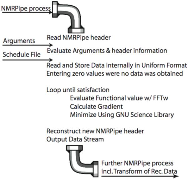
Flow diagram of FM reconstruction. See text for a description of the procedure.

The multidimensional minimization is delegated to the GSL Polak-Ribiere conjugate gradient algorithm, gsl_multimin_fdfminimizer_conjugare_pr. As the 1D, 2D and 3D FM reconstruction require 1D, 2D and 3D Fourier transforms respectively, FFTW is used for the 1D complex FFTs; 2D and 3D transforms are constructed of sets of 1D complex FFTs. The program allows reconstruction of up to three simultaneously sparsely sampled dimensions. This practically means support for 4D data as the direct dimension is processed separately by regular FFT via nmrPipe prior to FM reconstruction.

In addition to the main program, several supporting programs have been written. (1) A program, mpiPipe, was created in order to use MPI for delegating processing of approximately 1000 lines of C code (31,415 bytes). (2) Programs to convert from and to a “phase-first” internal format, phf2pipe (370 lines of C code) and pipe2phf (356 lines of C code). (3) Programs to reduce the data from US to NUS data by specified sampling schedule, used e.g. within the distill process.

The procedure of the mpiPipe program essentially achieves the following: (a) Initiating and connecting with the other processing nodes. (b) Receiving data according to NMRPipe specifications. (c) Once initiating is done, the head node engages each external processor with a job; (i) a task identifier is sent to the external processor, (ii) a static command operation is sent to the processor, (iii) a unique job order is assigned and kept, allowing asynchronous work flow, (iv) the data are prepared and sent, (v) a non-blocking receive is requested. (d) Once a processor node has completed its task, the head node receives it and new data are delegated. (e) Once all processed data have been received from the processing nodes, the processed data is moved from the internal storage to the output pipe according to NMRPipe specifications. Notable, the mpiPipe program may be used for most types of NMRPipe processing on a cluster or farm via MPI.

The phf2pipe was constructed, as it is customary to collect all phases for a particular sampling point before incrementing the sampling list when doing non-uniform sampling. For instance, in a 3D experiment each point of the hyper dimensional matrix consists of four FIDs: rr, ri, ir and ii, describing the four combinations of real (r) and imaginary (i) components of the two indirect dimensions. The internal format for NMRPipe typically requires a different layout of the data. Thus, the phf2pipe conversion is used after the multidimensional FM reconstruction. This results in a conventional NMRPipe data organization, which can be processed in a traditional and familiar fashion. The pipe2phf is a complementary program to phf2pipe, used within the distill process.

The program suite is implemented to run on a multiple cpu farm in parallel mode where the indirect data associated with each directly sampled data point are sent to one processor. Currently we use a farm of 32 Intel Xenon computers each containing four cores 3 GHz operating at 64 bit. Processing times are indicated for the spectra shown below. The program has also been ported on a ServMax Tesla GPU HPC, which contains a 3 GHz Intel CPU with a Nvidia CUDA 960-Core card.

Application of the FM reconstruction to 3D and 4D spectra of a large protein

The gain of resolution that can be obtained by NUS of triple resonance experiments is demonstrated with a 3D HNCO experiment on the 48 kDa C-domain of the non-ribosomal peptide synthetase EntF. Very high resolution can be obtained without extending the total measuring time compared to conventional linear sampling at low-resolution. This facilitates backbone resonances assignment of large proteins significantly. Figure 2 shows HN-C’ strips and sections of ¹H-¹⁵N planes of a 3D HNCO experiment on the 48 kDa C-domain of the non-ribosomal peptide synthetase EntF. Two experiments of the same overall measuring time are compared, using uniform (left) and non-uniform sampling (right). For both spectra 1250 indirect points were sampled. The spectrum on the left was obtained by recording the first 50 points in the nitrogen dimension and the first 25 points in the carbon dimension. For the spectrum on the right, the same number of increments (1250) was spread randomly over a Nyquist grid extending over 400 points in the nitrogen dimension and 100 points in the carbon dimension. Thus, while the Nyquist grid consists of 40,000 points, only 3% of the grid points were sampled. Comparison of the two spectra shows that spectrum of superior resolution can be obtained with non-uniform sampling. The H^N-C’ strips of the US spectrum (top left) exhibit numerous encroachments of peaks from adjacent planes due to the limited resolution in the ¹⁵N dimension. These encroachments are absent in the strips of the NUS high-resolution spectrum at the right. This is even more clearly demonstrated in the comparison of the ¹H-¹⁵N planes at the bottom of the figure. The increased resolution in the carbon dimension is clearly visible in the comparison of the strips in the two top panels. Thus, using NUS and FM reconstruction, very high-resolution spectra can be obtained in a reasonably short overall measuring time. This facilitates assignments and allows defining precise peak positions at the resolution provided by the high-field spectrometers.

Figure 2.

Comparison of two 3D semi constant time HNCO spectra of the 48 kDa C domain of EntF recorded with US (left) and NUS (right). Sampling points were selected randomly with an exponentially decreasing sampling density to account for relaxation. Top: Representative ¹H-¹³C’ strips. Bottom: representative sections of the H-N projections. For both spectra, a total of 1250 FIDs were recorded in the N-C Nyquist space, and thus the same measuring time was needed for both experiments. For the US spectrum, the first 50 and 25 grid points of the N-C Nyquist grid were populated, respectively; for the NUS spectrum, the 1250 recordings were randomly distributed over a much larger Nyquist grid spanned by 400 points in the nitrogen and 100 points in the carbon dimension. This represents population of only 3% of the 40,000 grid points. The NUS data were processed with the FM reconstruction procedure using 100 iterations minimizing the linear l₁ norm. Processing was carried out on a share 128 core Xenon cluster within 14 days. The dramatic gain in resolution is obvious.

The current FM reconstruction program can also handle 4D NUS spectra. Fig. 3 displays a small section of a ¹H-¹³C plane (ω₃ × ω₄) from a ¹³C-¹³C dispersed 4D NOESY of the 48 kDa C-domain of the non-ribosomal peptide synthetase EntF. Cross sections in all four dimensions are shown for the peak placed in a box at 0.47 ppm and 20.0 ppm, respectively. Here we call the finally frequency labeled ¹³C-¹H pair ¹H and ¹³C_dir, and the connected ¹³C-¹H pair ¹H_indir and ¹³C_indir. In the left panel all the missing points were reconstructed with the FM method using 100 cycles of conjugate gradient optimization. For comparison, in the right panel, the NUS spectrum was transformed with straight discrete Fourier transformation where all missing points were left at zero. As can be seen, the DFT method reproduces the strongest points, however, with a rather poor signal-to-noise ratio. In contrast, the FM reconstruction reveals well-defined and additional signals. Furthermore, the FM reconstruction lacks some false positive signals.

Figure 3.

FM reconstruction of a NUS 4D ¹³C-HSQC-NOESY-¹³C-HSQC spectrum of the 48 kDa C domain of the non-ribosomal peptide synthetase EntF. The sample is selectively protonated and ¹³C enriched for the methyls of Ile (δ-position), Leu and Val. 4000 complex points were sampled out of 24 (H_indir) × 16(C_indir) × 66(C_dir) = 25,344 complex points (16% sampling) for an experiment time of 7 days and 12 hours. The spectrum was recorded on an 800 μM sample on a Bruker 750 MHz spectrometer equipped with a cryoprobe. The experiment can be viewed as correlating proton/carbon pairs that are directly detected (H_dir/C_dir, for direct detected dimension) with other proton/carbon pairs (H_indir/C_indir) via nuclear Overhauser effects. The 2D plane shown is a ¹³C/¹H (ω₃/ω₄) section through the 4D cube. All 1D cross sections are through the peak marked by the box. FM reconstruction was carried out with seven minimization cycles minimizing the linear l₁ norm over eleven days, using a 128 core Xenon cluster, which was shared with other applications.

Application of the Distillation Procedure

To test the limits of NUS and FM reconstruction and to explore the effect of the distillation procedure we recorded a crowded 2D NOESY of the Gal11 KIX domain, a three-helix bundle protein with little NH chemical shift dispersion (Thakur et al., 2008). Fig. 4 (top) shows the spectrum recorded uniformly with 1024 increments. The spectrum in the middle was obtained with traditional random sampling of 384 of the 1024 points and processed with FM reconstruction. Here we sample the first 32 points linearly and the subsequent 352 points non-linearly with a random schedule following a uniformly weighted sampling probability. We call this a l32u schedule indicating that the first 32 indirect points were sampled linearly followed by the other points randomly picked but with uniform sampling density. As can be seen, the crowded central portion suffers from truncation artifacts leading to noise bands along the indirect dimension. The spectrum at the bottom was reconstructed with seven iterations of the distillation method. The reconstructed NUS spectrum is essentially identical to the US sampled spectrum although it was only recorded in one third of the time.

Fig. 4.

Effects of distillation in the FM reconstruction of a 2D NOESY spectrum of the Gal11 KIX domain. Top: 2D NOESY spectrum obtained at 600 MHz with 1024 complex increments in the t₁ dimension. Middle: The same data, from which 384 (3/8 of 1024) increments were selected on an “L32u” basis (the first 32 increments are sampled linearly, the succeeding 352 increments are randomly selected with uniform sampling density). Data were reconstructed with the FM algorithm. Processing time on a 128 cpu cluster using 500 iterations was 10 minutes. Bottom: Same data as in the middle with the addition of 7 iterations of the ad-hoc “distill” process. Processing time on a 128 cpu cluster was approximately one hour.

A comparison of US and NUS 3D ¹⁵N-dispersed NOESY spectra is shown in Fig. 5. In the NUS spectrum 32% of the indirect 2D time domain was sampled randomly. Here the NUS spectrum was recorded independently and not extracted from a US spectrum. Thus, some features are different, such as the spurious signals at the water position in the indirect ¹H dimension. The FM reconstructed spectrum was also run through the distill procedure and is compared with the regular FM reconstruction. The US and reconstructed NUS time domain data, with and without distillation, were then processed identically with NMRPipe. A representative ¹H-¹⁵N cross plane and a ¹H-¹H strip are compared in the figure. The spectra are essentially indistinguishable. Here, the sampling schedule was generated with a random number generator as described in (Rovnyak, Frueh et al., 2004). In this 3D NOESY, the distillation procedure yields only minor improvements compared to what it can do in the 2D NOESY shown in Fig. 4. Most significantly, the intensity of the diagonal peak is now identical to that in the US spectrum while it is somewhat decreased in the spectrum with the straight FM reconstruction without distillation.

Fig. 5.

Effect of the FM reconstruction on line shapes. We plot the values of the pixels of the FM reconstruction against the values of the same pixels from the linearly sampled data. If the line shape is reproduced exactly the correlation should be a straight line with slope 1 and a y-intercept of zero. We have analyzed a section of the 2D NOESY with a strong diagonal peak at the lower left corner of the 2D NOESY from Fig. 4. As can be seen, FM reconstruction only reproduces the line shapes with a slope of 0.897 and a y-intercept of 43771. Use of the distill procedure increases the slope to 0.947, and the y-intercept is reduced more than four fold.

Reproducibility of peak positions, peak intensities and line shapes

We have previously shown quantitatively and in much detail that the FM reconstruction reproduces peak intensities with high fidelity (Hyberts et al., 2007). We see no detectable changes of peak positions. To examine possible changes of line shapes we plot the values of the pixels of the FM reconstruction of the NUS data from Figure 4 against the values of the same pixels from the linearly sampled data (Figure 5A). If the line shape is reproduced exactly the correlation should be a straight line with slope 1 and a y intercept of zero. We have analyzed a section of the 2D NOESY with a strong diagonal peak, at the lower left corner of the 2D NOESY from Fig. 4. As can be seen, FM reconstruction only reproduces the line shapes with a slope of 0.897 and a y-intercept of 43771. Use of the distill procedure increases the slope to 0.947, and the y intercept is reduced more than four fold. Thus, the FM procedure provides a rather faithful reconstruction of line shapes, and distillation slightly improves the reproduction of the line shapes close to those obtained with uniform sampling.

Discussion

NUS offers the great advantage that multi-dimensional NMR spectra can be acquired at a resolution matching the spectrometer capabilities but without using excessive amounts of instrument time as would be needed for linearly stepping through the indirect dimensions towards the desirable maximum evolution times (Rovnyak, Hoch et al., 2004). To allow a faithful reconstruction of the spectra, we have developed the forward maximum entropy (FM) procedure. FM reconstruction obtains best approximations of the missing time-domain data points by using a high-dimensional conjugate gradient minimization of the norm of the frequency-domain data with respect to the missing data points. Currently the FM reconstruction software can handle up to three indirect dimensions (2D to 4D spectra). The speed of reconstruction depends on the size of the time-domain data grid and the complexity of the spectra. The spectra are most rapidly reconstructed using parallel mode on a multiple-cpu farm. An important benefit of the FM method is that it does not require setting of parameters and leads to a reconstructed time-domain data set that can be handled with any available processing software.

FM reconstruction of NUS triple resonance spectra is very robust and reproduces the spectra with high fidelity. Here the main benefit is that spectra can be recorded at very high resolution without the need of extra measurement time. This is particularly significant for large proteins where the higher resolution defines peak positions more accurately and facilitates cross peak assignments.

If spectra are very crowded and exhibit a wide dynamic range of peak intensities, such as encountered in 2D NOESYs with strong diagonals, regular FM reconstruction may lead to spurious bands along the indirect dimension. It is of paramount importance that the NOESY spectrum is reconstructed with high fidelity with respect to peak intensities. These intensities are directly used as distance constrains in structure calculations and the weak peaks generally provide the important long distance restrains which primarily determines the final structure. The quality of the FM reconstruction in this respect can be significantly improved with a distillation procedure that alleviates artifacts arising from very intense peaks. The distillation procedure is also most valuable “after the fact” once data were recorded, and it has been realized that the sampling schedule was not optimally chosen.

The FM reconstruction method, like other maximum entropy methods, does not infuse a model about line shapes. This is in contrast to linear prediction methods that assume Lorentzian line shapes. Thus, FM reconstruction is suitable for handling signals that have unusual shapes or are distorted due to spectrometer imperfections. It is perfectly usable, for example, to handle solid-state NMR spectra that contain powder patterns or other line shapes.

The FM procedure differs from other methods because it does not alter the points that are actually recorded. Other maximum entropy reconstructions, such as MaxEnt, vary all time domain data points, those not obtained and those obtained (Stern et al., 2002). In this case, an additional constraining term, C(t) = (t_i -t_i’)², is constructed in order not to stray too far from the original value of the recorded data. The set t’ = {t_i’} represents the back calculated trial spectrum. Summation is performed only over acquired data point indices. The constraining term is multiplied by a variable λ, often referred to as the LaGrange multiplier, and the final term is added to the target function, Q’(f) = −S(f) + λ C(t). Note that the target function in the MaxEnt approach is written partially in the frequency domain, and partially in the time domain. The issue however with traditional MaxEnt is that it seems non-trivial to algorithmically resolve the constraining term at the end of the minimization. The term is therefore left, and the solution depends on the value chosen for λ. Practically, this is manifested in a non-linearity response in the reconstruction of the signal intensities (Schmieder et al., 1997a). Since Maximum Entropy Methods do not take account of a correlation between a collection of data points, such as in form of a line shape, this non-linearity is also the reason why finite lines are often sharpened by traditional MaxEnt. In contrast to the FM reconstruction, MaxEnt requires setting of the parameters λ and def. High values of λ in traditional MaxEnt increase the linearity at the cost of computational time; low values of λ shorten the computation but make tall peaks taller and small peaks smaller. A theoretical value of infinity would yield that the minimization only takes the constraining term C in account, enforcing the values that were obtained to stay the same, not necessarily optimizing the non obtained values; a value of zero releases the attachment to the term C, resulting in S to be optimized without regards to obtained data and sets the spectrum to a straight line. The MaxEnt algorithm has been applied successfully, for example when used for triple resonance experiments of well-behaved proteins (Rovnyak, Frueh et al., 2004). It has weaknesses, however, with processing spectra with a high dynamic range and may lose weak peaks. The latter aspect has motivated the development of the FM reconstruction procedure. In addition, in MaxEnt the user needs to make a choice for the parameters λ and def. Furthermore, and in contrast to the FM approach, MaxEnt delivers a frequency-domain spectrum. Thus, the user can/must do all processing in the same MaxEnt software package.

It has been pointed out that NUS spectra can be reconstructed by a straightforward discrete Fourier transformation (DFT), and an example is shown in Fig. 3. This creates significant truncation noise. Nevertheless, straightforward DFT of NUS spectra may be suitable if one is only interested in determining the chemical shifts of the strongest peaks at high resolution. However, it goes to the expense of losing weak signals, and the S/N is severely affected (see Fig. 3). In contrast, the FM reconstruction procedure can provide high resolution chemical shifts, an optimal S/N and high fidelity intensities even for small peaks.

Conclusion

The FM reconstruction procedure has evolved to be used routinely for reconstructing spectra with up to three NUS indirect dimensions. It is straightforward to use for triple-resonance experiments and allows a dramatic increase of the resolution without the need of extra long measurement times. For crowded data and spectra with a high dynamic range it can be combined with a distillation procedure described here. The outcome of FM reconstruction of NUS data depends crucially on the choice of optimal sampling schedules. This has been discussed extensively in the literature, together with a whole array of reconstruction methods. A further analysis of optimizing sampling schedules is under development and will be discussed in detail elsewhere. NUS with FM reconstruction is particularly beneficial for large proteins where the approach facilitates unambiguous peak assignments.

Fig. 6.

Comparison of sections of a NUS and FM reconstructed 3D ¹⁵N dispersed NOESY with the corresponding US experiment. Both spectra cover a Nyquist grid of 128 and 50 indirect time domain points in the indirect ¹H and ¹⁵N dimensions, respectively. For the NUS data 2048 grid points (32%) were selected randomly, and the missing time-domain data were obtained with the FM reconstruction. The direct dimension was processed to 512 t₃ data points prior to the FM reconstruction of the indirect dimensions. The US data were processed with regular FM and also with 7 iterations of distillation. All three data sets, the US, NUS-FM, and NUS-FM-distill time domain data were finally transformed identically with the DFT algorithm of the NMRPipe program. Top left: ¹H-¹⁵N HSQC as a reference. Bottom: Comparison of the same cross plane from the US data, the NUS-FM reconstructed data, and the same NUS data reconstructed with the FM and distillation procedure. Top right: ¹H-¹H strips from the same three data sets. The positions where the cross planes are taken are indicated with arrows. The FM reconstruction of the NUS spectrum was obtained in 1.5 hrs on a 128 cpu Linux farm. The US and NUS spectra were recorded independently, the NUS spectrum was recorded in one third of the time.

References

- Barna JCJ, Laue ED, Mayger MR, Skilling J, Worrall SJP. Exponential sampling, an alternative method for sampling in two-dimensional NMR experiments. J Magn Reson. 1987;73:69–77. [Google Scholar]
- Chylla RA, Markley JL. Theory and application of the maximum likelihood principle to NMR parameter estimation of multidimensional NMR data. J Biomol NMR. 1995;5:245–258. doi: 10.1007/BF00211752. [DOI] [PubMed] [Google Scholar]
- Coggins BE, Venters RA, Zhou P. Filtered backprojection for the reconstruction of a high-resolution (4,2)D CH3-NH NOESY spectrum on a 29 kDa protein. J Am Chem Soc. 2005;127:11562–11563. doi: 10.1021/ja053110k. [DOI] [PubMed] [Google Scholar]
- Coggins BE, Zhou P. Polar Fourier transforms of radially sampled NMR data. J Magn Reson. 2006;182:84–95. doi: 10.1016/j.jmr.2006.06.016. [DOI] [PubMed] [Google Scholar]
- Coggins BE, Zhou P. High resolution 4-D spectroscopy with sparse concentric shell sampling and FFT-CLEAN. J Biomol NMR. 2008;42:225–239. doi: 10.1007/s10858-008-9275-x. [DOI] [PMC free article] [PubMed] [Google Scholar]
- Daniell GJ, Hore PJ. Maximum entropy and NMR - a new approach. J. Magn. Reson. 1989;84:515–536. [Google Scholar]
- Delaglio F, Grzesiek S, Vuister GW, Zhu G, Pfeifer J, Bax A. NMRPipe: a multidimensional spectral processing system based on UNIX pipes. J Biomol NMR. 1995;6:277–293. doi: 10.1007/BF00197809. [DOI] [PubMed] [Google Scholar]
- Frueh DP, Sun ZY, Vosburg DA, Walsh CT, Hoch JC, Wagner G. Non-uniformly Sampled Double-TROSY hNcaNH Experiments for NMR Sequential Assignments of Large Proteins. J Am Chem Soc. 2006;128:5757–5763. doi: 10.1021/ja0584222. [DOI] [PMC free article] [PubMed] [Google Scholar]
- Gull S, Skilling J. MEMSYS5 Quantified Maximum Entropy. 1991 [Google Scholar]
- Gutmanas A, Jarvoll P, Orekhov VY, Billeter M. Three-way decomposition of a complete 3D 15N-NOESY-HSQC. J Biomol NMR. 2002;24:191–201. doi: 10.1023/a:1021609314308. [DOI] [PubMed] [Google Scholar]
- Hoch JC. Modern spectrum analysis in nuclear magnetic resonance: alternatives to the Fourier transform. Methods Enzymol. 1989;176:216–241. doi: 10.1016/0076-6879(89)76014-6. [DOI] [PubMed] [Google Scholar]
- Hoch JC, Stern AS. NMR data processing. Wiley-Liss; New York, NY: 1996. [Google Scholar]
- Högbom Aperture synthesis with a non-regular distribution of interferometer baselines. Astron. Astrophys. Suppl. 1974;15:417–426. [Google Scholar]
- Hyberts SG, Heffron GJ, Tarragona NG, Solanky K, Edmonds KA, Luithardt H, Fejzo J, Chorev M, Aktas H, Colson K, Falchuk KH, Halperin JA, Wagner G. Ultrahigh-Resolution (1)H-(13)C HSQC Spectra of Metabolite Mixtures Using Nonlinear Sampling and Forward Maximum Entropy Reconstruction. J Am Chem Soc. 2007;129:5108–5116. doi: 10.1021/ja068541x. [DOI] [PMC free article] [PubMed] [Google Scholar]
- Kazimierczuk K, Kozminski W, Zhukov I. Two-dimensional Fourier transform of arbitrarily sampled NMR data sets. J Magn Reson. 2006;179:323–328. doi: 10.1016/j.jmr.2006.02.001. [DOI] [PubMed] [Google Scholar]
- Kazimierczuk K, Zawadzka A, Kozminski W, Zhukov I. Random sampling of evolution time space and Fourier transform processing. J Biomol NMR. 2006;36:157–168. doi: 10.1007/s10858-006-9077-y. [DOI] [PubMed] [Google Scholar]
- Kim S, Szyperski T. GFT NMR, a new approach to rapidly obtain precise high-dimensional NMR spectral information. J Am Chem Soc. 2003;125:1385–1393. doi: 10.1021/ja028197d. [DOI] [PubMed] [Google Scholar]
- Korzhneva DM, Ibraghimov IV, Billeter M, Orekhov VY. MUNIN: application of three-way decomposition to the analysis of heteronuclear NMR relaxation data. J Biomol NMR. 2001;21:263–268. doi: 10.1023/a:1012982830367. [DOI] [PubMed] [Google Scholar]
- Kupce E, Freeman R. Projection-reconstruction technique for speeding up multidimensional NMR spectroscopy. J Am Chem Soc. 2004a;126:6429–6440. doi: 10.1021/ja049432q. [DOI] [PubMed] [Google Scholar]
- Kupce E, Freeman R. Fast reconstruction of four-dimensional NMR spectra from plane projections. J Biomol NMR. 2004b;28:391–395. doi: 10.1023/B:JNMR.0000015421.60023.e5. [DOI] [PubMed] [Google Scholar]
- Marion D. Fast acquisition of NMR spectra using Fourier transform of non-equispaced data. J Biomol NMR. 2005;32:141–150. doi: 10.1007/s10858-005-5977-5. [DOI] [PubMed] [Google Scholar]
- Orekhov VY, Ibraghimov I, Billeter M. Optimizing resolution in multidimensional NMR by three-way decomposition. J Biomol NMR. 2003;27:165–173. doi: 10.1023/a:1024944720653. [DOI] [PubMed] [Google Scholar]
- Orekhov VY, Ibraghimov IV, Billeter M. MUNIN: a new approach to multi-dimensional NMR spectra interpretation. J Biomol NMR. 2001;20:49–60. doi: 10.1023/a:1011234126930. [DOI] [PubMed] [Google Scholar]
- Rovnyak D, Frueh DP, Sastry M, Sun ZY, Stern AS, Hoch JC, Wagner G. Accelerated acquisition of high resolution triple-resonance spectra using non-uniform sampling and maximum entropy reconstruction. J Magn Reson. 2004;170:15–21. doi: 10.1016/j.jmr.2004.05.016. [DOI] [PubMed] [Google Scholar]
- Rovnyak D, Hoch JC, Stern AS, Wagner G. Resolution and sensitivity of high field nuclear magnetic resonance spectroscopy. J Biomol NMR. 2004;30:1–10. doi: 10.1023/B:JNMR.0000042946.04002.19. [DOI] [PubMed] [Google Scholar]
- Schmieder P, Stern AS, Wagner G, Hoch JC. Application of nonlinear sampling schemes to COSY-type spectra. J Biomol NMR. 1993;3:569–576. doi: 10.1007/BF00174610. [DOI] [PubMed] [Google Scholar]
- Schmieder P, Stern AS, Wagner G, Hoch JC. Improved resolution in triple-resonance spectra by nonlinear sampling in the constant-time domain. J Biomol NMR. 1994;4:483–490. doi: 10.1007/BF00156615. [DOI] [PubMed] [Google Scholar]
- Schmieder P, Stern AS, Wagner G, Hoch JC. Quantification of maximum-entropy spectrum reconstructions. J Magn Reson. 1997a;125:332–339. doi: 10.1006/jmre.1997.1117. [DOI] [PubMed] [Google Scholar]
- Schmieder P, Stern AS, Wagner G, Hoch JC. Quantification of maximum-entropy spectrum reconstructions. J Magn Reson. 1997b;125:332–339. doi: 10.1006/jmre.1997.1117. [DOI] [PubMed] [Google Scholar]
- Shannon CE. A Mathematical Theory of Communication. Bell System Technical Journal. 1948;27:379–432. 623–656. [Google Scholar]
- Shimba N, Stern AS, Craik CS, Hoch JC, Dotsch V. Elimination of 13Calpha splitting in protein NMR spectra by deconvolution with maximum entropy reconstruction. J Am Chem Soc. 2003;125:2382–2383. doi: 10.1021/ja027973e. [DOI] [PubMed] [Google Scholar]
- Stern AS, Li KB, Hoch JC. Modern spectrum analysis in multidimensional NMR spectroscopy: comparison of linear-prediction extrapolation and maximum-entropy reconstruction. J Am Chem Soc. 2002;124:1982–1993. doi: 10.1021/ja011669o. [DOI] [PubMed] [Google Scholar]
- Sun ZJ, Hyberts SG, Rovnyak D, Park S, Stern AS, Hoch JC, Wagner G. High-resolution aliphatic side-chain assignments in 3D HCcoNH experiments with joint H-C evolution and non-uniform sampling. J, Biomol. NMR. 2005;32:55–60. doi: 10.1007/s10858-005-3339-y. [DOI] [PubMed] [Google Scholar]
- Sun ZY, Frueh DP, Selenko P, Hoch JC, Wagner G. Fast assignment of 15N-HSQC peaks using high-resolution 3D HNcocaNH experiments with non-uniform sampling. J Biomol NMR. 2005;33:43–50. doi: 10.1007/s10858-005-1284-4. [DOI] [PubMed] [Google Scholar]
- Thakur JK, Arthanari H, Yang F, Pan SJ, Fan X, Breger J, Frueh DP, Gulshan K, Li DK, Mylonakis E, Struhl K, Moye-Rowley WS, Cormack BP, Wagner G, Naar AM. A nuclear receptor-like pathway regulating multidrug resistance in fungi. Nature. 2008;452:604–609. doi: 10.1038/nature06836. [DOI] [PubMed] [Google Scholar]
- Tugarinov V, Kay LE, Ibraghimov I, Orekhov VY. High-resolution four-dimensional 1H-13C NOE spectroscopy using methyl-TROSY, sparse data acquisition, and multidimensional decomposition. J Am Chem Soc. 2005;127:2767–2775. doi: 10.1021/ja044032o. [DOI] [PubMed] [Google Scholar]
- Venters RA, Coggins BE, Kojetin D, Cavanagh J, Zhou P. (4,2)D Projection--reconstruction experiments for protein backbone assignment: application to human carbonic anhydrase II and calbindin D(28K) J Am Chem Soc. 2005;127:8785–8795. doi: 10.1021/ja0509580. [DOI] [PubMed] [Google Scholar]