Cognitive Mechanisms Underlying Risky Decision-Making in Chronic Cannabis Users

Abstract

Chronic cannabis users are known to be impaired on a test of decision-making, the Iowa Gambling Task (IGT). Computational models of the psychological processes underlying this impairment have the potential to provide a rich description of the psychological characteristics of poor performers within particular clinical groups. We used two computational models of IGT performance, the Expectancy-Valence Learning model (EVL) and the Prospect-Valence Learning model (PVL), to assess motivational, memory, and response processes in 17 chronic cannabis abusers and 15 control participants. Model comparison and simulation methods revealed that the PVL model explained the observed data better than the EVL model. Results indicated that cannabis abusers tended to be under-influenced by loss magnitude, treating each loss as a constant and minor negative outcome regardless of the size of the loss. In addition, they were more influenced by gains, and made decisions that were less consistent with their expectancies relative to non-using controls.

Substance abusers often are impaired on laboratory measures of decision-making (Bechara et al., 2001; Petry, 2003; Petry, Bickel, & Arnett, 1998; Rogers et al., 1999). For example, in a laboratory decision-making task known as the Iowa Gambling Task (IGT; Bechara, Damasio, Damasio, & Anderson, 1994), substance abusers often make choices that lead to small, immediate gains at the cost of larger losses over time (S. Grant, Contoreggi, & London, 2000). Cannabis (marijuana) users, like other substance-using populations, perform more poorly than non-using controls on the IGT (Lamers, Bechara, Rizzo, & Ramaekers, 2006; Whitlow et al., 2004), even after prolonged abstinence from the drug (Bolla, Eldreth, Matochik, & Cadet, 2005). This impairment may be due to underlying deficits or differences in psychological processes (e.g., memory impairments, loss insensitivity, etc.), but pinpointing such processes can be difficult with traditional behavioral measures from the IGT. Recent work has attempted to disentangle component processes of the IGT by means of computational cognitive models (Busemeyer & Stout, 2002; Garavan & Stout, 2005; Yechiam, Busemeyer, Stout, & Bechara, 2005). In this report, we use mathematical models of choice behavior on the IGT to better understand the risk taking behavior of cannabis users. We present a comparison of two such models, and then compare estimated model parameters of chronic cannabis users and controls to identify the particular psychological processes which may be impaired in cannabis users.

For the IGT, the participant must make a series of choices from four decks of cards with the goal of maximizing his or her net payoff across trials. On each trial, the participant selects a card from any of the four decks and is informed how much (s)he won or lost by choosing that card. Every choice leads to a gain that sometimes is coupled with a simultaneous loss (see Table 1). Selecting from the two “disadvantageous” decks will result in a larger per-selection gain, but on average leads to a net loss over ten selections, whereas selecting from the two “advantageous” decks results in a smaller per-selection gain but an overall net gain over ten selections. To perform well on the IGT the participant learns to select primarily from advantageous decks on the basis of the net gains and losses they experience across the task. Thus, the IGT incorporates cognitive (i.e., learning and memory) and motivational processes (i.e., responsivity to gains and losses) associated with the anticipation of outcomes following choices over time. The decision to use or abstain from also drugs invokes processes related to learning from previous experiences with the drug, and the perceived rewards (i.e., pleasure) and punishments (i.e., financial, interpersonal, legal trouble) associated with drug use.

Table 1.

Payoffs used in the Iowa Gambling Task

Deck	Win per card	Losses	Expected value per selection
A (Disadvantageous)	$100	Probability = 0.5 to lose $150, $200, $250, $300, or $350 (Frequent)	−$25
B (Disadvantageous)	$100	Probability = 0.1 to lose $1250 (Infrequent)	−$25
C (advantageous)	$50	Probability = 0.2 to lose $25 or $75; Probability = 0.3 to lose $50 (Frequent)	+$25
D (advantageous)	$50	Probability = 0.1 to lose $250 (Infrequent)	+$25

Computational cognitive models allow us to disentangle the processes contributing to IGT performance and to identify specifically those processes which may account for the poorer overall performance of an individual or group on the task (Busemeyer & Stout, 2002). Our research group has developed a mathematical model called the Expectancy Valence Learning (EVL) model (Busemeyer & Stout, 2002) to investigate the psychological processes underlying individuals’ decisions on the IGT. The model has three assumptions. First, a utility function represents an individual’s subjective evaluation of gains and losses. Second, a learning rule allows the development of expectancies for each deck that are updated on the basis of experienced utilities. Third, these expectancies determine the probabilities that the participant will choose a given deck on each trial via a choice rule. The EVL model is based on principles derived from the judgment and decision-making literature and yields theoretically-derived dependent measures (model parameters) that describe psychological processes underlying IGT performance. These parameters reflect the degree to which the decision maker attends to gains versus losses (Attention to Gains parameter), his or her learning rate (Recency parameter), and the degree of consistency between deck selections and the expected outcomes associated with each deck (Consistency parameter). By applying the model to several datasets from clinical populations who demonstrate impaired IGT performance, we have identified distinctive patterns within the empirical data which differentiate various groups of drug abusers, subjects with Huntington’s disease, and subjects with orbitofrontal brain lesions from their respective control groups (for a review, see Yechiam et al., 2005).

Using the EVL model of IGT performance, our group has shown previously that disruptions in psychological processes may underlie the poorer performance of cocaine abusers (Stout, Busemeyer, Lin, Grant, & Bonson, 2004) and polysubstance abusers (Stout, Rock, Campbell, Busemeyer, & Finn, 2005) on the IGT. With regard to cannabis users specifically, a recent analysis of decision processes in a sample of 21 young (mean age = 24 years) cannabis-using college students found no significant differences between that group and non-using controls on any EVL model parameters (Bishara et al., in press). In addition, a review of the EVL modeling of the IGT performance in various clinical samples included a brief summary of 25 chronic cannabis abusers who differed from controls on the Recency and Attention to Gains parameters (Yechiam et al., 2005). This report includes the 17 chronic cannabis abusers from that report who had been abstinent only long enough for the acute effects of the drug to have worn off (i.e., they were no longer intoxicated, or high) but before they would have started having withdrawal symptoms, and extends this previous work principally by allowing an evaluation of a new model that may have better explanatory ability for IGT behavior.

Investigations of cognition among chronic cannabis abusers have identified disruptions in psychological processes which could contribute to their poorer IGT performance. For instance, chronic users are impaired relative to non-users on neuropsychological measures of memory and learning (for reviews, see I. Grant, Gonzalez, Carey, Natarajan, & Wolfson, 2003; Solowij & Battisti, 2008). This impairment could compromise their ability to maintain and update representations of the expectancy for each deck across IGT trials. The effects of chronic cannabis use on sensitivity to reward and punishment are less clear, although acute administration studies have shown that cannabis exposure is associated with increased risk-taking and decreased sensitivity to choice outcomes (Lane & Cherek, 2002; Lane, Cherek, Tcheremissine, Lieving, & Pietras, 2005). These results are supported by a recent functional magnetic resonance imaging (fMRI) study which showed that chronic cannabis users exhibit patterns of neural activity consistent with hypersensitivity during reward anticipation and hyposensitivity to loss outcomes (Nestor, Hester, & Garavan, in press). Chronic users may show a similar pattern of behavior on the IGT, manifested as a bias toward the disadvantageous decks. Lastly, chronic cannabis users score highly on personality measures related to risk-seeking, which may lead them to make impulsive selections that are inconsistent with their expectancies regarding deck outcomes (Satinder & Black, 1984).

We recently developed the Prospect Valence Learning (PVL) model, which is a modification of the EVL model (Ahn, Busemeyer, Wagenmakers, & Stout, 2008)¹. The PVL model employed in this report uses the same learning rule as the EVL model, but uses a different utility function and a different choice rule. Ahn et al. (2008) showed that the PVL model resulted in better post-hoc fits, simulation performance, and generalizability than comparison models when applied to IGT data from healthy normal subjects. There are two main purposes of this report. The primary purpose is to compare the new PVL model to the EVL model using both a clinical population and a control population for the first time. This is an important step for two reasons: first, we need to determine whether the superior predictive power of the PVL model over the EVL models continues to hold for clinical populations; second, we need to examine if the parameters estimated from the PVL model are more or less informative than the parameters estimated from the EVL model with respect to revealing important differences between clinical and control populations.

The equations for the EVL and PVL models are shown in Table 2. The models explain choices in the IGT in slightly different ways. First consider the concept ‘valuing a card’ shown in Table 2. As each card is selected in the IGT, the decision maker assesses the value of that card. The decision maker’s valuation of a card will vary depending on the relative amount of attention the (s)he pays to gains versus losses. Some individuals will only register gains, others will only register losses, and still others will attend to both wins and losses, with the weighting of attention varying across decision-makers. The Attention to Gains parameter (w; see Table 2) in the EVL model captures the relative amount of attention a decision maker pays to gains compared to losses on a given trial. If w = 0 all attention is paid to losses, whereas if w = 1 all attention is paid to gains. Based on the level of attention to gains, the decision maker generates a value for that card. In the PVL model, the subjective utilities are represented by a non-linear prospect utility function. The shape parameter (α) governs the curvature of the utility function (0 < α < 1: as α approaches 1, subjective utility increases in direct proportion to the outcome value; as α approaches 0, subjective utility increases in a stepwise fashion so all gains are subjectively equal and all losses are subjectively equal). The utility function of the PVL model also contains a loss-aversion parameter (λ) which indicates the subject’s sensitivity to losses compared to gains (0 < λ < 10: as λ approaches 0 losses are experienced as neutral events with utility = 0; for λ = 1 losses and gains have the same impact; for λ > 1 losses have greater impact than gains on the subjective utility of an outcome, leading to loss aversion). The advantage of using the PVL’s non-linear utility function is that it accounts for the gain/loss frequency effect. That is, winning $100 five times is often perceived as better than winning $500 once, even though the net gain is equivalent (Erev & Barron, 2005). The EVL’s linear utility function assumes that both of these events have the same overall utility. Therefore, the PVL model explains participants’ preferences for decks with low net-loss frequency (e.g., Deck B) over decks with high net-loss frequency (e.g., Deck A) even if their expected values are the same (Ahn et al., 2008).

Table 2.

EVL and PVL model equations for estimating parameters. Model-fitting selects parameter values that maximize the likelihood of the decision maker’s responses, given the model.

Concept	Model	Model Equation	Free Parameter(s)
Valuing a card	EVL	u(t) = w · win(t) − (1 − w) · loss(t)	w = Attention to Gains
	PVL	$u(t)=\{\begin{array}{rr}\hfill x{(t)}^a& \hfill \text{if}x(t)\ge 0\\ \hfill -\lambda \mid x(t){\mid }^a& \hfill \text{if}x(t)<0\end{array}$	λ = Loss Aversion α = Utility Shape
Creating a deck expectancy, E, for decky j on trial t	EVL & PVL	Ej = Ej(t − l) + A · δj(t) · [u(t) − Ej(t−1)]	A = Recency
Probability of choosing Deck j	EVL & PVL	$Pr[D(t+1)=j]=\frac{e^{\theta (t)·E_j(t)}}{{\displaystyle \sum _{j=1}^4}{e}^{\theta (t)·E_j(t)}}$
Consistency between choices and expectancies	EVL	$\theta (t)={\left(\frac{t}{10}\right)}^c$	c = Consistency
	PVL	θ(t) = 3c − 1

Note. j refers to deck A, B, C, or D. The variable δ_jt is a dummy variable equal to 1 if deck j was chosen on trial t, otherwise 0.

Next consider the concept ‘creating an expectancy’ shown in Table 2. With the experience of each card’s payoff, the decision maker can then revise the expectancy about the deck from which the card was chosen. Each time a new card is drawn, the old deck expectancy is updated based on the value of the new card. The Recency parameter (A) is a parameter of the delta learning rule (Rescorla & Wagner, 1972) for both the EVL and PVL models. The Recency parameter (0 < A < 1) is an index of learning rate, indicating how much weight is given to past experiences with a given deck versus how much weight is placed on the value of the most recent selection from that deck. A high Recency parameter indicates that the value of the most recent card selection has a large influence on the expectancy for that deck, and forgetting of previous card selections is rapid. In contrast, a low Recency parameter indicates that the value of the most recent card selection has a small influence on the expectancy for that deck, and forgetting is more gradual. In this way, expectancies about each deck develop as each new card is selected.

The third concept in Table 2 is the ‘probability of choosing a deck.’ In order to select a deck on each trial, the decision maker compares the current expectancies for each deck. A good decision maker makes choices consistent with his or her deck expectancies as the trials progress and as confidence in the expectancies increases with experience. The Consistency parameter (c) is an indicator of the fidelity between the decision maker’s selections and expectancies as the task progresses. A high value indicates that the decision maker’s choices are deterministic, resulting in maximal choices from the deck with the highest expectancy. A low Consistency value indicates that the decision maker chooses more randomly, possibly reflecting impulsivity or boredom with the task. The EVL model uses a trial-dependent choice rule in which the consistency increases or decreases over trials (−5 < c < 5; Busemeyer & Stout, 2002). In contrast, the PVL model uses a trial-independent choice rule in which consistency remains constant over trials (0 < c < 5).

In summary, for the current study, we applied the EVL and PVL models to the IGT performance data obtained from 17 chronic, heavy cannabis users and 15 control subjects who had only minimal lifetime exposure to cannabis. Empirical results from ten of the subjects in this sample were included in a previous report (Whitlow et al, 2004), which revealed poor gambling task performance in the cannabis group as compared to the control group. We replicate this finding in an enlarged sample of chronic cannabis users. We then report a comparison of the ability of the EVL and PVL models to account for each group’s performance on the IGT. Finally, we present an analysis of the individual differences in psychological processes underlying cannabis users’ poor performance on the IGT.

Methods

Participants

Participants consisted of 17 chronic cannabis users and 15 control subjects (see Table 3). Inclusion in the chronic cannabis group required reported cannabis usage for at least 25 out of every 30 days for at least 5 years. This group reported an average of 13.2 ± 9.0 (M ± SD) years of cannabis abuse. The control group included individuals who reported a maximum of 100 lifetime uses of cannabis, with no use in the past year. On average, they reported 19.7 ± 29.4 lifetime uses of cannabis. Thus, the control group had minimal lifetime cannabis exposure (Pope, Gruber, & Yurgelun-Todd, 1995; Pope & Yurgelun-Todd, 1996). Potential subjects were excluded based on reported history of head trauma, neurological disorders, psychiatric disorders (including substance abuse disorders other than cannabis in the cannabis group), and systemic diseases which might affect the central nervous system. All participants gave written informed consent.

Table 3.

Mean values on demographic measures. Standard deviations are in parentheses.

	Group
	Controls (n = 15)	Cannabis users (n = 17)
Age (years)	29.6 (7.6)	33.3 (8.2)
Education (years)	14.9 (2.5)	13.7 (1.8)
Estimated IQ	110 (10.9)	101.2 (13.8)
Drinks/week	2.9 (4.2)	4.3 (6.3)
Cigs./day	8.3 (10.1)	12.2 (8.7)
Age at first cannabis use (years)	18.6 (5.0)	16.4 (5.4)
Years of cannabis use	-	13.2 (9.0)

Members of the chronic cannabis user group were asked to abstain from cannabis use for 12 hours prior to the study. We expected twelve hours to be long enough to avoid any effects of acute intoxication and short enough to precede significant withdrawal symptoms (Budney, Moore, Vandrey, & Hughes, 2003; Grotenhermen, 2003). Among users, the last reported cannabis use averaged 13.9 ± 2.3 (M ± SD) hours prior to testing and ranged from 11 to 18 hours prior to testing. Abstinence was confirmed by urine drug screens (Laboratory Corporation of merica, Research Triangle Park, NC). The presence of symptoms related to depression, anxiety, and alcohol use disorders were assessed via the Beck Depression Inventory-II (BDI-II; Beck, Steer, & Brown, 1996), Spielberger State-Trait Anxiety Inventory (STAI; Spielberger, 1983) and the Alcohol Use Disorders Identification Test (AUDIT; Bohn, Babor, & Kranzler, 1995), respectively. Users did not significantly differ from controls on years of education, gender distribution, number of cigarettes smoked per day, number of alcoholic drinks consumed per week, or scores on the BDI-II, STAI, or AUDIT (all ps > .05; see Table 3). However, the difference in estimated full-scale IQ was marginally significant between the groups (estimated IQ [M ± SD] for controls = 110 (10.9); users = 101.2 (13.8); t(30) = 1.99; p = .06).

Procedures

Subjects participated in a study that included a brief neuropsychological battery (described in Whitlow et al., 2004) prior to completion of the IGT. The IGT was administered while subjects underwent fMRI; however, only the behavioral results are analyzed in this report.

The procedures for the IGT have been described in detail previously by Bechara and colleagues (Bechara et al., 1994), and are described only briefly here. Subjects began the task with $2000 in play gambling money. They were told that the purpose of the game was to win as much play money as possible, and that the subject who accumulated the largest amount over the course of the study would win a real monetary bonus of $50. This bonus was intended to motivate subjects to perform well on the task. The IGT was presented on a computer display, and subjects made a series of 100 card selections from four decks of cards labeled A, B, C, and D by pressing one of four buttons on a button box. Choosing a card from deck A or B always yielded a gain of $100, whereas choosing a card from deck C or D always yielded a gain of $50. Each deck was associated with a schedule of penalties, such that some card selections yielded both a gain and a loss. Every 10 cards selected from deck A or B resulted in a net loss of $250 whereas every 10 cards selected from deck C or D resulted in a net gain of $250 (see Table 1). Thus, the advantageous decks C and D provided smaller gains but also smaller losses relative to the disadvantageous decks A and B. Following each selection, the computer displayed the gain and, if present, the loss for that selection and also displayed total earnings. For each subject, all 100 card selections were recorded.

Results

Analysis of IGT Performance

To analyze IGT performance, the 100 card selections were divided into a series of five blocks. Blocks 1 through 4 each consisted of twenty card selections (trials 1–20, 21–40, 41–60, and 61–80, respectively) whereas Block 5 consisted of fifteen card selections (trials 81 through 95). Performance for trials 96 through 100 was not analyzed because many subjects depleted at least one of the 4 decks between the 96^th and 100^th trial, changing the structure of the task at that point from a choice among 4 decks to a choice among 3 decks. The percentage of advantageous choices was computed for each block. A 2 (group: User v. Control) × 5 (Block) repeated measures analysis of (ANOVA) was performed to examine group differences in learning across blocks. In addition, we conducted similar analyses to contrast group preferences for specific decks across blocks.

IGT Performance

Although Controls and Users began the IGT by selecting predominantly from the disadvantageous decks, only Controls subsequently learned to select from the advantageous decks (see Figure 1). Controls made more advantageous selections than Users as the task progressed (F_BlockxGroup [4,120] = 3.44, p < .05). Follow-up ANOVAs revealed that Controls outperformed Users on Blocks 2 through 5 of the IGT (ps < .01) and exhibited a trend toward better performance in Block 1 (p = .06). These results are consistent with previous reports indicating impaired IGT performance among chronic cannabis users (Bolla et al., 2005; Lamers et al., 2006; Whitlow et al., 2004). The groups differed in their preference for specific decks throughout the task (F_{DeckxBlockxGroup} [7.2, 215.3] = 3.73, p < .001 [degrees of freedom corrected using the Greenhouse–Geisser correction for violated sphericity]; see Figure 2). The most popular decks among all participants were Decks B and D (infrequent punishment; disadvantageous and advantageous, respectively). Compared to Controls, Users made significantly more selections from Deck B in blocks 2 and 5 and fewer selections from Deck D in blocks 2 through 5 (all ts > 2.43; ps < .05).

Figure 1.

IGT performance for controls and cannabis users, by block. Dots represent mean proportion of advantageous selections in each block; error bars represent ± 1 SEM. Controls outperformed Users on Blocks 2 – 5 (p < .01).

Figure 2.

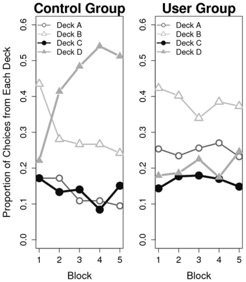
Comparison of group selections from each deck across each block of the IGT.

Model Evaluation

To determine which model to use in comparing control and user groups, two methods were used to evaluate the EVL and the PVL: post-hoc model fits and simulation performance of each model.

Post-hoc model fits

First, maximum likelihood estimates of the parameters from each model were obtained by searching for parameters that minimized the following lack of fit function (see Busemeyer & Stout, 2002). Define Y_i(t) as column vector with Y_ij(t) = 1 if deck j was chosen on trial t, otherwise zero. Define X_i(t) as another vector containing the payoffs received by subject i on trial t. Define

$$Pr[D(t)=j\mid Y_i(t-1),X_i(t-1),\dots ,Y_i(1),X_i(1)],$$ (1)

as the probability of choosing deck j to be selected on trial t by a model given information from subject i on all previous trials. Define the lack of fit function for model m as

$${G^2}_{i,m}=-2·{\sum }_{t=2,t}{\sum }_{j=1,4}{Y}_{ij}(t)·ln\{Pr[D(t)=j\mid Y_i(t-1),\dots ,Y_i(1),X_i(1)]\},$$ (2)

where t = the total number of trials. The search to minimize the lack of fit function was done using a Nelder-Mead algorithm and multiple quasi-random starting points.

The EVL and PVL models were compared separately to a Bernoulli baseline model using the Bayesian Information Criterion (BIC; Schwartz, 1978) to adjust for differences in the number of parameters (model complexity).

$${\text{BIC}}_{i,m}={G^2}_{i,m}+k_m\ast ln(N-1),$$ (3)

where N equals the total number of trials (in this case, 95) and k_m equals the number of model parameters for model m. The BICs that we report are the BICs produced by the taking the differences with respect to baseline: (BIC_Baseline − BIC_EVL) and (BIC_Baseline − BIC_PVL). Thus positive values indicate improvement of a model (either EVL or PVL) over the baseline. The Bernoulli model assumes that a participant’s probability of selecting from a specific deck on a given trial is equal to the final proportion of cards the decision maker actually selected from that deck. For example, if a participant’s proportion of cards selected from each deck were p(Deck A) = .10, p(Deck B) = .30, p(Deck C) = .10 and p(Deck D) = .50, then the Bernoulli model posits that this person has the same .50 probability of selecting from Deck D on all trials.

The model comparison analyses produced discrepant results for the Control and User groups. Non-parametric sign tests revealed that the PVL model fit significantly better than the EVL model among Controls (PVL median BIC relative to Bernoulli model = 1.24, EVL median BIC relative to Bernoulli model = −9.43; p < .001). However, the EVL model fit significantly better than the PVL model among Users (PVL median BIC relative to Bernoulli model = −6.70, EVL median BIC relative to Bernoulli model = −3.32; p < .05). Overall, both the EVL and PVL models provided a poor fit for Users’ data. However, we focus our analyses on the differences between the groups on the PVL model parameters for the following reasons. First, the PVL and EVL models assume learning across trials. Users on average did not exhibit learning during the IGT as revealed by a non-significant effect of Block on the proportion of advantageous choices for that group, F(4, 64) = .99, n.s. (see Figure 1). Therefore, since Users’ preference for disadvantageous decks remained relatively consistent over the course of the task, it is unsurprising that the Bernoulli model fit Users’ data better than the PVL and EVL models.

Second, Users’ tendency to overvalue gains while discounting losses resulted in utility functions that were approximately linear when generated by both the PVL and EVL models (see Figure 4a). Under the EVL model, Users’ Attention to Gains parameter was very high (median w =.96), while under the PVL model their Loss Aversion (λ) parameter was very low and their Utility Shape parameter (α) was very high (see below). These values represent a special case whereby the utility function of the PVL model mimics that of the EVL model. However, the PVL model’s extra free parameter relative to the EVL model means that the PVL model was penalized to a greater extent than the EVL when the BIC was calculated. Indeed, nonparametric sign tests revealed that the G² values for both models relative to the Bernoulli model were similar in both the Control and User groups, ps > .10.

Figure 4.

Subjective median utility values for a) net gains only, and b) net losses only, plotted separately for Users (solid lines) and Controls (dashed lines). Dotted lines are ± 1 SEM and dots are possible outcomes in the IGT.

Third, we conducted a hierarchical Bayesian analysis to verify that the PVL model provided a better fit for the data than the Bernoulli model when all subjects from both groups were used for Bayesian model comparison (see Appendix). This analysis produced strong evidence favoring the PVL model over the Bernoulli model (Bayes factor = 29). This suggests that the PVL model generalizes better to both groups than the Bernoulli model, and that the PVL parameter estimates for Users may still be validly interpreted to explain their behavior, even if its model fit to the user group data alone may not be as good as the Bernoulli model’s.

Fourth, the results of simulation analyses (see below) supported the superiority of the PVL over the EVL with regard to the ability of the models to accurately simulate the actual choice behavior of each group. These results are similar to those of Ahn et al. (2008), which showed that the prospect utility function had better accuracy and generalizability than the expectancy utility function when accounting for participants’ choices on the IGT.

Simulation method

A simulation method can be used to evaluate how accurately the model is able to predict a participant’s future choice behavior given that individual’s previous choices and the outcomes (s)he obtained from those choices. Using the procedure in Appendix B of Ahn et al. (2008), we ran simulations using both models. For each model, a subject’s best fitting parameters were provided to the model and 100 simulations of that subject’s trial by trial deck selections were created. The simulated proportion selected from each deck was then computed separately for users versus controls.

Examination of Figure 3 suggests that the PVL model more accurately simulated the observed pattern of choices for each group. Among Controls, the EVL simulation over-predicts the proportion actually chosen from the high frequency loss decks (A and C) and under-predicts the proportion chosen from the low frequency loss decks (B and D). In contrast, the PVL simulation better matches participants’ actual preferences for the low frequency loss decks (B and D). Among Users, the PVL does a better job than the EVL of modeling Users’ actual preference for high immediate gains coupled with low frequency losses (Deck B). The remaining results will focus on the PVL model.

Figure 3.

Simulation results of the PVL and EVL models for a) Control group and b) user group. Error bars represent ± 1 SEM.

Predicting Group Membership using Model Parameters

We evaluated the ability of the parameters of the PVL model to significantly predict group membership after accounting for group differences in estimated IQ and IGT behavioral performance using logistic regression. This analysis, with group (User v. Control) as the dependent variable, revealed that the PVL model parameters significantly improved the accuracy of logistic regression model to predict group membership. The model containing only estimated IQ and IGT performance (percent advantageous) as predictors classified 84.4% of participants correctly (χ²(2) = 21.96; p < .001; −2 log likelihood = 22.28, sensitivity (to cannabis use) = 88.2%, specificity = 80%). After accounting for IQ and IGT performance, the inclusion of the PVL model parameters to the logistic regression model significantly improved the ability to predict group membership (χ²(4) = 11.66; p < .05; −2 log likelihood = 10.62, sensitivity = 100%, specificity = 93.3%). The logistic regression model classified 96.9% of participants correctly with the inclusion of the PVL parameters.

Between-groups Comparison of PVL Model Parameters

Next, we compared the groups on the parameter estimates of the PVL model to determine how psychological processes relevant to decision-making differed between Users and Controls. The groups differed significantly on all parameters generated by the PVL model. Non-parametric group comparisons were used because the model parameters were not normally distributed (see Table 4). Compared to Controls, Users exhibited lower values for the Consistency (Mann-Whitney U_c = 37.0; p < .001) and Loss Aversion (U_λ = 47.0; p < .01) parameters, but higher values for the Recency (U_A = 60.5; p < .01) and Utility Shape (U_α = 54.5; p < .01) parameters.

Table 4.

Median values of model parameters for the PVL model.

	Recency (A)**	Utility shape (α)**	Loss Aversion (λ)**	Consistency (c)***
Controls	.06	.44	.73	1.64
Users	.21	.99	.01	.88

Note. Groups were compared using the Mann-Whitney U test.

^**p < .01;

^***p < .001

Users and Controls differed in their subjective evaluations of the outcomes experienced during the IGT as shown by plots of their utility functions for gains (Figure 4a) and losses (Figure 4b). To construct these plots, we first computed a utility function for each subject based upon his or her Utility Shape (α) and Loss Aversion (λ) values as determined by the PVL model. Next, the average utility function for members of each group was generated by averaging group members’ expected utility values associated with each of a number of possible actual outcomes. In Figure 4, the x-axis of each graph corresponds to the actual (objective) amount gained/lost on a trial and the y-axis to the subjective utility of the outcome as calculated by the prospect utility function. Compared to Controls, Users appeared to be more sensitive to gains but less sensitive to losses. The difference in subjective utility between gains of $50 and $100 was approximately $50 for Users but only $30 for Controls (Figure 4a). For large losses (−$1250), the subjective utility was approximately $0 for Users but −$400 for Controls (Figure 4b). Thus, Controls were less sensitive to the magnitudes of gains, whereas Users were less sensitive to the magnitude of losses. Users’ utility functions were so extreme for losses that loss magnitude typically was ignored altogether.

Discussion

Summary of basic findings

The results of the present study suggest that the PVL model provides a more accurate account of decision-making on the IGT than the EVL model, and demonstrate the usefulness of the PVL model in uncovering the cognitive processes that contribute to performance on that task.

Furthermore, the results show that the PVL model may be used to identify specific impairments in those processes among members of a clinical sample (chronic cannabis users). The between-groups comparison of the PVL model parameters indicated that Users and Controls differed on several processes germane to decision-making. Relative to Controls, Users’ choices on the IGT were characterized by greater sensitivity to gains, insensitivity to losses, greater dependence upon recent outcomes, and less consistency with expected payoffs. Thus, cannabis users differ from controls in terms of the motivational, memory, and response processes that contribute to overall performance on the IGT (Stout et al., 2004).

Comparison of decision processes between cannabis users and controls

The present findings suggest that psychological processes important for decision-making may be disrupted in chronic cannabis users. The implications of such disruptions and the relationship between the present results and the existing literature on cognition and cannabis abuse are discussed in detail below.

Sensitivity to Gains and Losses

Our results suggest that chronic cannabis users are relatively insensitive to losses and exhibit an attentional bias, compared to controls who are more loss-averse. Examination of Figure 4a reveals that Users were more sensitive than Controls to increases in the magnitude of wins, while Figure 4b shows that Users were relatively insensitive to increases in the magnitude of losses. These results are consistent with previous research demonstrating a relationship between substance abuse, increased reward salience, and decreased sensitivity to punishment (Finn, Mazas, Justus, & Steinmetz, 2002). In addition, these results are similar to those obtained in previous studies of decision-making in cocaine and polysubstance users using the EVL model (Stout et al., 2004; Stout et al., 2005). The IGT performance of those groups was characterized by heightened attention to gains relative to losses. Thus, chronic cannabis abusers may exhibit the same hypersensitivity to gains and/or hyposensitivity to losses as do chronic users of other drugs such as cocaine.

In addition to the IGT, drug users’ hypersensitivity to gains has been observed with other tasks and models. Drug users have shown increased risk taking behavior on both the Balloon Analog Risk Task (Lejuez et al., 2002) and the Angling Risk Task (Pleskac, 2008). When these tasks were further analyzed with a Bayesian learning model, drug use was related to higher sensitivity to payoffs, as indicated by the model’s γ⁺ parameter (Pleskac, 2008; Wallsten, Pleskac, & Lejuez, 2005). Thus, the finding of a higher alpha parameter in marijuana users here converges with findings from other tasks and models, and thereby provides support for the usefulness of the PVL model.

The PVL model’s use of the prospect utility function may explain why that model fit the data better than did the EVL model. The PVL model incorporates two parameters (α, λ) that collectively describe sensitivity to gains and loss aversion, whereas the EVL model computes outcome utilities based upon a single parameter (w). Indeed, sensitivity to gains and loss aversion may not be perfectly correlated (i.e., an individual could be sensitive to losses and gains, whereas another could be sensitive to losses only). The PVL model permits this type of relationship, whereas the EVL model treats win/loss sensitivity as perfectly correlated, such that an increase in sensitivity to losses is necessarily accompanied by a decrease in sensitivity to gains. Importantly, the simulation data revealed that the PVL model was able to account for participants’ preferences for Deck B, whereas the EVL model was not (Figure 3). This may be a consequence of the PVL model’s non-linear utility function, rather than its extra model parameter. Yechiam and Busemeyer (2005) modified the EVL model to incorporate a linear two-parameter utility function (including separate gain/loss sensitivity parameters) but with the same learning rule (delta learning rule) and choice rule (trial-dependent choice rule) as in the present study. The results revealed that the modified EVL model was unable to predict participants’ preferences for Deck B.

Previous research has indicated that acute cannabis exposure may increase human participants’ sensitivity to reward in a decision-making task. Lane and colleagues (2005) showed that individuals were more likely to choose a “risky” option over a “non-risky” option following exposure to cannabis versus placebo. In that study, the “non-risky” option was associated with lower per-selection gains but a positive expected value over the experimental session (112 trials), whereas the “risky” option was associated with higher per-selection gains but an expected value of $0 over 112 selections. Furthermore, following the highest dose of marijuana administered during the study, participants were more likely to perseverate on the risky option whether they won or lost. In contrast, participants in the placebo condition exhibited a higher probability to shift to the non-risky option when a risky choice resulted in punishment. The IGT is similar to the task used by Lane and colleagues (2005) in that both tasks require participants to consider outcomes experienced over a sequence of selections when making choices between options associated with varying outcomes. The present results suggest that chronic cannabis abuse may be associated with disruptions in motivational processes similar to those observed during acute intoxication.

Recency

Users exhibited a higher value for the Recency parameter than did Controls, suggesting that the decisions of Users were affected more heavily by recent outcomes than were those of the Controls. Large values of this parameter indicate rapid forgetting of past outcomes. In addition, IGT performance suffers when a working memory load is introduced (Hinson, Jameson, & Whitney, 2002). Thus, working memory impairment among chronic cannabis users may compromise their ability to retain active representations of previous outcomes on the IGT, resulting in poorer overall task performance.

The present results differ from previous studies from our group that modeled substance users’ decision-making on the IGT. Bishara and colleagues (in press) found no differences between young cannabis users and non-using controls on any EVL model parameters, although that sample was younger than our User group (mean age = 24 years v. 33 years, respectively) and were generally lighter users of cannabis. In a separate investigation, Stout and colleagues (2004) found that male cocaine users did not differ with regard to the learning rate parameter when compared to sex-matched controls, whereas Stout and colleagues (2005) found that female (but not male) polysubstance users exhibited higher values for that parameter². Collectively, these results suggest that different drugs of abuse may be associated with different outcomes on assessments of learning and memory processes. In addition, they suggest that sex differences may exist among substance users with regard to relationships between chronic drug use and learning and memory processes.

Our modeling analysis is consistent with previous reports that have identified an association between cannabis use and poorer performance on measures of learning and memory (I. Grant et al., 2003; Solowij & Battisti, 2008). There are at least two possible accounts of Users’ memory impairment and its impact on decision-making on the IGT. First, Users may have had trouble explicitly recalling the previous outcomes of their choices, which may have led them to choose more often from disadvantageous decks. Second, users may have been unable to integrate the information obtained from each card selection (i.e., the card’s value) online as it was presented into an overall expectancy of the outcomes associated with each deck. That is, users may have been unable to retain the outcome associated with each selection in memory long enough to integrate it into a coherent representation of the deck’s value that could be used to guide selections toward advantageous decks.

Consistency

Users exhibited a lower value for the Consistency parameter than Controls, indicating that Users’ selections were less consistent with their expectancies regarding the outcomes associated with each deck. Group differences on this parameter may reflect differences in personality variables related to risk-seeking. Current and former substance users score higher than non-users on personality measures designed to assess impulsivity (Allen, Moeller, Rhoades, & Cherek, 1998; Patton, Stanford, & Barratt, 1995). Cannabis-using college students rate more highly than non-users on a self-report measure of disinhibition (Satinder & Black, 1984), a personality trait associated with a tendency to seek out and engage in risky experiences. Among adolescents, cannabis use is correlated with engagement in risky behaviors, such as sexual promiscuity (Miles et al., 2001). Thus, cannabis users may possess underlying personality traits that predispose them to engage in multiple forms of risky behavior in addition to substance use. With regard to the present findings, Users’ lower value for the Consistency parameter may reflect the tendency of this group to engage in risk-seeking behavior, regardless of whether they are aware of the potential consequences. That is, on the IGT, heavy cannabis users may understand the contingencies associated with each deck but may choose from the disadvantageous decks because they are undeterred by their association with risk.

Caveats

The results of the present investigation should be viewed in light of some potential caveats. We studied a small sample of users that had been using for a long period of time (M = 13.2 years); therefore, these results may not generalize to individuals that have used cannabis for a shorter period of time. In addition, Users’ performance may have reflected the presence of transient levels of cannabinoids in the brain rather than persistent alterations of neural structures underlying decision-making that are the result of chronic exposure to cannabis (Pope et al., 1995). Cannabis metabolites can be detected in the urine of chronic users even following one month abstinence from the drug (Ellis, Mann, Judson, Schramm, & Tashchian, 1985), and the effects of these metabolites on cognition are unclear.. Furthermore, the present study’s cross-sectional design and use of self-selected (instead of randomly assigned) samples of Users and Controls limit our ability to determine whether the observed group differences in IGT performance and PVL model parameters reflect the effects of drug use, or premorbid group differences in personality traits or cognitive-motivational processes. For instance, cannabis users are more impulsive than non-users (Satinder & Black, 1984), a personality trait which has been associated with poorer IGT performance (Davis, Patte, Tweed, & Curtis, 2007). Future research on this topic may be best informed by modeling the decision making processes of groups of participants that are matched on impulsivity or other relevant personality traits but that differ in terms of their exposure to drugs of abuse, or by within-subjects designs which compare the decision-processes of substance users during a period when they are actively using with the same processes in those individuals after a period of prolonged abstinence.

Overall evidence for the PVL model was strong compared to the Bernoulli baseline model (see Appendix), but group comparisons revealed that the PVL model fit Users’ data poorly. Given Users’ poor learning on the IGT, however, the baseline model’s better fit for this group is unsurprising (see Figure 1). We may view this from the perspective of model mimicry, which is not uncommon in mathematical modeling (Navarro, Pitt, & Myung, 2004; Wagenmakers, Ratcliff, Gomez, & Iverson, 2004). Model mimicry occurs when competing models provide a similar level of fit to a certain kind of data pattern. This problem may be resolved if it can be shown that one model describes a wider range of plausible data than the other. Otherwise, it may be necessary to evaluate those models using other kinds of criteria such as interpretability. In the present case, we may view that the baseline model mimics the PVL model for Users’ data. The utility of the PVL model to explain individual differences in choice behavior on the IGT would be in question if the baseline model mimicked the PVL model for most of the observed data patterns, but the maximum likelihood and hierarchical Bayesian analyses demonstrate that this is not the case. Furthermore, the PVL model resulted in a plausible, interpretable set of model parameters for both groups, and Users’ parameters were consistent with previous research on the cognitive sequelae of chronic cannabis use. Therefore, the PVL model may provide a useful account of decision-making on the IGT even in clinical groups that do not perform well on that task.

Conclusions

Our analyses revealed that the PVL model of decision-making more accurately accounted for participants’ behavior on the IGT than did the original EVL model. This may be due to the PVL model’s use of a prospect utility function, which can account for the gain/loss frequency effect and Controls’ decreasing sensitivity to very large gains versus smaller gains (Ahn et al, 2008). We found that chronic cannabis users’ decisions on the IGT could be characterized by more reward-seeking, less loss-aversion, greater reliance upon recent outcomes, and less consistency between choice behavior and outcome expectancies than non-users. These results support the contention that chronic cannabis users exhibit impairments on psychological processes related to motivation, learning and memory, and behavioral control. These impairments may contribute to poor decision-making in this group and lead to or exacerbate problems related to cannabis use, such as the inability to achieve or maintain abstinence. Future investigations should focus on the similarities and differences among these psychological processes across diverse substance-abusing samples. Collectively this knowledge may contribute to the development of prevention and intervention approaches for substance use disorders that are sensitive to individual differences in specific psychological processes underlying decision-making.

Appendix

Understanding differences in basic decision making processes between drug abusers and non abusers using cognitive models such as EVL and PVL relies on estimating model parameters from individual subjects (using maximum likelihood methods), and comparing competing non-nested cognitive models using a model comparison index. This method requires us to collect a large number of trials from each participant. In practice, however, the actual number of trials we may collect from each participant is small, which may contribute to noisy parameter estimates for each person. One could assume that all people in the group are the same, and average across individuals and fit the model to more stable data representing the average individual. However, there are substantial individual differences (i.e., the behavior of the average does not look like any single individual’s behavior), and fitting the average data can produce highly misleading results (Estes & Maddox, 2005). A hierarchical Bayesian analysis may be applied to avoid these problems (cf. Gelman, Carlin, Stern, & Rubin, 2004; Gill, 2008) and using this approach yields a substantial increase in power to detect differences and identify relationships. Hierarchical Bayesian analysis allows for individual differences yet pools information from the data of all individuals to obtain more stable and reliable estimates of model parameters.

We developed a hierarchical Bayes extension of the PVL model as follows. Rather than fitting each individual separately using maximum likelihood, this analysis used Bayesian estimation based on data from all individuals. In particular, we use a distribution model to represent the individual differences in model parameters (rather than fitting individuals separately). A beta distribution is used to represent the distribution of individual differences for each of the four parameters. Specifically, if we randomly sample an individual i, A_i ~ beta (μ_A, σ_A), α_i ~ beta (μ_α, σ_α), λ_i ~ beta (μ_λ, σ_λ), and c_i ~ beta (μ_c, σ_c), jointly independent, where μ and σ are the mean and standard deviation of each beta distribution. This is a commonly used distribution for Bayesian modeling when the parameters are bounded. It is effective because it is capable of capturing a wide variety of distribution shapes. The Bayesian approach to estimation also requires an assignment of a prior distribution to the mean and standard deviation of each beta distribution. For the prior distribution, we use a uniform (i.e., flat) distribution which assumes no a priori knowledge about these parameters. Finally, the observed data matrix from all participants is used to compute the posterior distributions for all parameters according to the Bayes rule. For each model parameter, the posterior distributions describe the likelihood that various values correspond to the true parameter value. This entire procedure was implemented in the WinBUGS environment (Lunn, Thomas, Best, & Spiegelhalter, 2000)^A1.

Table A1 summarizes the results from the hierarchical Bayes estimation of the PVL model parameters. For each group, the parameter estimate in the table is the posterior mean of the group average of individual parameters (i.e., mean of beta distribution discussed in the preceding paragraph). Differences between control and user groups were evaluated by examining the posterior distribution of differences of group means. For example, from the hierarchical Bayes estimation, a posterior distribution of group mean difference of the recency parameter (i.e.,μ_A.control − μ_A.user) can be obtained. Then, by estimating the probability of this value being greater than (or less than) zero, we can estimate the posterior probability that the group mean parameter of a group is greater or less than that of the other. Figure A1 shows such posterior distributions of the group mean difference of each parameter. The results from the hierarchical Bayes analysis, including the group means of each parameter and their differences between groups, are consistent with the results obtained from the maximum likelihood estimation procedure (see Table 4).

Table A1.

Posterior mean values of group mean parameters for the PVL model.

	Recency (A)**	Utility shape (α)**	Loss Aversion (λ)***	Consistency (c)***
Controls	.05	.39	1.12	1.73
Users	.27	.89	.04	.81

Note. In this Bayesian analysis, groups are compared by computing the posterior probability that each parameter of a group is greater than that of another group. Thus, the p values listed below do not have the same meaning as the p values in traditional hypothesis testing, but should be interpreted as direct estimates of such probabilities.

^**p < .005;

^***p < .0001

Figure A1.

Posterior distributions of differences of group mean parameters. Differences represent each mean parameter of the control group minus the corresponding parameter of the user group. Specifically, they are denoted by μ_{A control} − μ_A.user, μ_α.control − μ_α.user, μ_λ.control − μ_λ.user, and μ_{c control} − μ_c.user. Each of the parameters is the mean of the beta distribution that models individual differences in each PVL model parameter for the two groups.

A benefit of hierarchical Bayes modeling lies not only in the estimation of model parameters but also in model comparison. The inference of model selection can also be affected by noise in the data if done solely with individual data, just as with parameter estimation. With non-hierarchical models, the best that can be done is to obtain as many model selection indexes, such as BIC values, as the number of individual subjects, and then to perform a significance test of the null hypothesis that two competing models are equally plausible. By assuming that individual data are totally independent, however, this approach loses the power of the test. Hierarchical modeling, in contrast, properly accumulates evidence in the data by capturing the dependency among individuals, if it exists.

The same hierarchical form of the PVL model as described above was used in the present hierarchical Bayes analysis of model comparison. For the baseline model, a categorical distribution with four fixed probabilities (i.e., the probability of a choice from each of the four decks) was specified to explain each subject’s responses throughout all trials. Two assumptions were made to convert this into to a hierarchical form. First, this set of probabilities was assumed to be different among subjects; second, those probabilities were assumed to be governed by a parent distribution for which a Dirichlet distribution with diffuse priors for the Dirichlet parameters was used. Data from all subjects were used to estimate the posterior probability of the PVL model being true versus the Bernoulli baseline model. An equal probability of 0.5 for each model was assumed as a prior. Initially, two separate analyses were performed using control and user group data, just as with the case of parameter inference. The results showed that the posterior probability of the PVL model against the Bernoulli model, evidenced by the data, is approximately 1 − (10¹⁸) for the control group, and 0.000012 for the user group. These values translate into the more commonly used Bayes factors of 87 for Controls and −23 for Users on the scale of twice the natural logarithm. Both are considered to be “very strong” evidence according to the guidelines suggested by Kass and Raftery (1995), and agree with the results of the non-hierarchical BIC analyses conducted for each group separately that are described in the main text.

Theoretically, however, there is not much to learn from modeling if the conclusion is that the PVL model explains people’s learning in the control group better whereas the baseline model fits users’ behavior better. The reason is that a model that provides a good description for data from a population should, if it is to be considered to be a good one, do so for data from another population as well. That is, the PVL model should generalize adequately well to users’ data even if its model fit may not be as good as that of a competing model, and the same logic applies to the baseline model, too, if it is to be considered to be a good model. A straightforward way to compare these models in this regard is to perform the same Bayesian model comparison described above, but using all subjects’ data from both groups to select the model that generalizes better across all individuals. The results of this analysis produced a Bayes factor of 29, indicating very strong evidence for the PVL model and the superior generalizability of that model to all participants as compared to the baseline model.

References

- Ahn WY, Busemeyer JR, Wagenmakers EJ, Stout JC. Comparison of decision learning models using the generalization criterion method. Cognitive Science. 2008;32:1376–1402. doi: 10.1080/03640210802352992. [DOI] [PubMed] [Google Scholar]
- Allen TJ, Moeller FG, Rhoades HM, Cherek DR. Impulsivity and history of drug dependence. Drug and Alcohol Dependence. 1998;50:137–145. doi: 10.1016/s0376-8716(98)00023-4. [DOI] [PubMed] [Google Scholar]
- Bechara A, Damasio AR, Damasio H, Anderson SW. Insensitivity to future consequences following damage to human prefrontal cortex. Cognition. 1994;50:7–15. doi: 10.1016/0010-0277(94)90018-3. [DOI] [PubMed] [Google Scholar]
- Bechara A, Dolan S, Denburg N, Hindes A, Anderson SW, Nathan PE. Decision-making deficits, linked to a dysfunctional ventromedial prefrontal cortex, revealed in alcohol and stimulant abusers. Neuropsychologia. 2001;39:376–389. doi: 10.1016/s0028-3932(00)00136-6. [DOI] [PubMed] [Google Scholar]
- Beck AT, Steer RA, Brown GK. Beck Depression Inventory. 2. San Antonio, TX: Psychological Corporation; 1996. (BDI-II) [Google Scholar]
- Berger JO. Statistical decision theory and Bayesian analysis. 2. New York: Springer-Verlag; 1985. [Google Scholar]
- Bishara AJ, Pleskac TJ, Fridberg DJ, Yechiam E, Lucas J, Busemeyer JR, Finn PR, Stout JC. Similar processes despite divergent behavior in two commonly used measures of risky decision-making. Journal of Behavioral Decision Making. 2009;22:435–454. doi: 10.1002/bdm.641. [DOI] [PMC free article] [PubMed] [Google Scholar]
- Bohn MJ, Babor TF, Kranzler HR. The Alcohol Use Disorders Identification Test (AUDIT): Validation of a screening instrument for use in medical settings. Journal of Studies on Alcohol. 1995;56:423–432. doi: 10.15288/jsa.1995.56.423. [DOI] [PubMed] [Google Scholar]
- Bolla KI, Eldreth DA, Matochik JA, Cadet JL. Neural substrates of faulty decision-making in abstinent marijuana users. Neuroimage. 2005;26:480–492. doi: 10.1016/j.neuroimage.2005.02.012. [DOI] [PubMed] [Google Scholar]
- Budney AJ, Moore BA, Vandrey RG, Hughes JR. The time course and significance of cannabis withdrawal. Journal of Abnormal Psychology. 2003;112(3):393–402. doi: 10.1037/0021-843x.112.3.393. [DOI] [PubMed] [Google Scholar]
- Busemeyer JR, Stout JC. A contribution of cognitive decision models to clinical assessment: Decomposing performance on the Bechara Gambling Task. Psychological Assessment. 2002;14(3):253–262. doi: 10.1037//1040-3590.14.3.253. [DOI] [PubMed] [Google Scholar]
- Davis C, Patte K, Tweed S, Curtis C. Personality traits associated with decision-making deficits. Personality and Individual Differences. 2007;42(2):279–290. [Google Scholar]
- Ellis GM, Mann MA, Judson BA, Schramm NT, Tashchian A. Excretion patterns of cannabinoid metabolites after last use in a group of chronic users. Clinical Pharmacology and Therapeutics. 1985;38(5):572–578. doi: 10.1038/clpt.1985.226. [DOI] [PubMed] [Google Scholar]
- Estes WK, Maddox WT. Risks of drawing inferences about cognitive processes from model fits to individual versus average performance. Psychonomic Bulletin and Review. 2005;12(3):403–408. doi: 10.3758/bf03193784. [DOI] [PubMed] [Google Scholar]
- Erev I, Barron G. On adaptation, maximization, and reinforcement learning among cognitive strategies. Psychological Review. 2005;112(4):912–931. doi: 10.1037/0033-295X.112.4.912. [DOI] [PubMed] [Google Scholar]
- Finn PR, Mazas CA, Justus AN, Steinmetz J. Early-Onset Alcoholism With Conduct Disorder: Go/No Go Learning Deficits, Working Memory Capacity, and Personality. Alcoholism: Clinical and Experimental Research. 2002;26(2):186–206. [PubMed] [Google Scholar]
- Garavan H, Stout JC. Neurocognitive insights into substance abuse. Trends in Cognitive Sciences. 2005;9:195–201. doi: 10.1016/j.tics.2005.02.008. [DOI] [PubMed] [Google Scholar]
- Grant I, Gonzalez R, Carey CL, Natarajan L, Wolfson T. Non-acute (residual) neurocognitive effects of cannabis use: A meta-analytic study. Journal of the International Neuropsychological Society. 2003;9:679–689. doi: 10.1017/S1355617703950016. [DOI] [PubMed] [Google Scholar]
- Grant S, Contoreggi CS, London ED. Drug abusers show impaired performance in a laboratory test of decision making. Neuropsychologia. 2000;38:1180–1187. doi: 10.1016/s0028-3932(99)00158-x. [DOI] [PubMed] [Google Scholar]
- Grotenhermen F. Pharmacokinetics and Pharmacodynamics of Cannabinoids. Clinical Pharmacokinetics. 2003;42(4):327–360. doi: 10.2165/00003088-200342040-00003. [DOI] [PubMed] [Google Scholar]
- Hinson JM, Jameson TL, Whitney P. Somatic markers, working memory, and decision making. Cognitive, Affective, & Behavioral Neuroscience. 2002;2:341–353. doi: 10.3758/cabn.2.4.341. [DOI] [PubMed] [Google Scholar]
- Kass RE, Raftery AE. Bayes factors. Journal of the American Statistical Association. 1995;90:773–795. [Google Scholar]
- Lamers CTJ, Bechara A, Rizzo M, Ramaekers JG. Cognitive function and mood in MDMA/THC users, THC users and non-drug using controls. J Psychopharmacol. 2006;20(2):302–311. doi: 10.1177/0269881106059495. [DOI] [PubMed] [Google Scholar]
- Lane SD, Cherek DR. Marijuana effects on sensitivity to reinforcement in humans. Neuropsychopharmacology. 2002;26(4):520–529. doi: 10.1016/S0893-133X(01)00375-X. [DOI] [PubMed] [Google Scholar]
- Lane SD, Cherek DR, Tcheremissine OV, Lieving LM, Pietras CJ. Acute marijuana effects on human risk taking. Neuropsychopharmacology. 2005;30:800–809. doi: 10.1038/sj.npp.1300620. [DOI] [PubMed] [Google Scholar]
- Lejuez CW, Read JP, Kahler CW, Richards JB, Ramsey SE, Stuart GL, Strong DR, Brown RA. Evaluation of a behavioral measure of risk taking: The Balloon Analogue Risk Task (BART) Journal of Experimental Psychology: Applied. 2002;8(2):75–84. doi: 10.1037//1076-898x.8.2.75. [DOI] [PubMed] [Google Scholar]
- Lunn DJ, Thomas A, Best N, Spiegelhalter D. WinBUGS - A Bayesian modelling framework: Concepts, structure, and extensibility. Statistics and Computing. 2000;10:325–337. [Google Scholar]
- Miles DR, van den Bree MBM, Gupman AE, Newlin DB, Glantz MD, Pickens RW. A twin study on sensation seeking, risk taking behavior and marijuana use. Drug and Alcohol Dependence. 2001;62:57. doi: 10.1016/s0376-8716(00)00165-4. [DOI] [PubMed] [Google Scholar]
- Navarro DJ, Pitt MA, Myung IJ. Assessing the distinguishability of models and the informativeness of data. Cognitive Psychology. 2004;49:47–84. doi: 10.1016/j.cogpsych.2003.11.001. [DOI] [PubMed] [Google Scholar]
- Nestor L, Hester R, Garavan H. Increased ventral striatal BOLD activity during non-drug reward anticipation in cannabis users. Neuroimage. doi: 10.1016/j.neuroimage.2009.07.022. (in press) [DOI] [PMC free article] [PubMed] [Google Scholar]
- Patton JH, Stanford MS, Barratt ES. Factor structure of the Barratt Impulsiveness Scale. Journal of Clinical Psychology. 1995;51(6):768–774. doi: 10.1002/1097-4679(199511)51:6<768::aid-jclp2270510607>3.0.co;2-1. [DOI] [PubMed] [Google Scholar]
- Petry NM. Discounting of money, health, and freedom in substance abusers and controls. Drug and Alcohol Dependence. 2003;71:133–141. doi: 10.1016/s0376-8716(03)00090-5. [DOI] [PubMed] [Google Scholar]
- Petry NM, Bickel WK, Arnett M. Shortened time horizons and insensitivity to future consequences in heroin addicts. Addiction. 1998;93(5):729–738. doi: 10.1046/j.1360-0443.1998.9357298.x. [DOI] [PubMed] [Google Scholar]
- Pleskac TJ. Decision making and learning while taking sequential risks. Journal of Experimental Psychology: Learning, Memory, & Cognition. 2008;34:167–185. doi: 10.1037/0278-7393.34.1.167. [DOI] [PubMed] [Google Scholar]
- Pope HG, Gruber AJ, Yurgelun-Todd DA. The residual neuropsychological effects of cannabis: The current status of research. Drug and Alcohol Dependence. 1995;38:25–34. doi: 10.1016/0376-8716(95)01097-i. [DOI] [PubMed] [Google Scholar]
- Pope HG, Yurgelun-Todd DA. The residual cognitive effects of heavy marijuana use in college students. Journal of the American Medical Association. 1996;275(7):521–527. [PubMed] [Google Scholar]
- Rescorla RA, Wagner AR. A theory of Pavlovian conditioning: Variations in the effectiveness of reinforcement and nonreinforcement. In: Black AH, Prokasy WF, editors. Classical Conditioning II. Appleton-Century-Crofts; 1972. pp. 64–99. [Google Scholar]
- Rogers RD, Everitt BJ, Baldacchino A, Blackshaw AJ, Swainson R, Wynne K, et al. Dissociable deficits in the decision-making cognition of chronic amphetamine abusers, opiate abusers, patients with focal damage to prefrontal cortex, and tryptophan-depleted normal volunteers: Evidence for monoaminergic mechanisms. Neuropsychopharmacology. 1999;20:322–339. doi: 10.1016/S0893-133X(98)00091-8. [DOI] [PubMed] [Google Scholar]
- Satinder KP, Black A. Cannabis use and sensation-seeking orientation. Journal of Psychology. 1984;116(1):101. doi: 10.1080/00223980.1984.9923623. [DOI] [PubMed] [Google Scholar]
- Schwartz G. Estimating the dimension of a model. Annals of Statistics. 1978;5:461–464. [Google Scholar]
- Solowij N, Battisti R. The chronic effects of cannabis on memory in humans: A review. Current Drug Abuse Reviews. 2008;1:81–98. doi: 10.2174/1874473710801010081. [DOI] [PubMed] [Google Scholar]
- Spielberger CD. Manual for the State-Trait Anxiety Inventory (STAI) Palo Alto, CA: Consulting Psychologists Press; 1983. [Google Scholar]
- Stout JC, Busemeyer JR, Lin A, Grant SR, Bonson KR. Cognitive modeling analysis of the decision-making processes in cocaine abusers. Psychonomic Bulletin & Review. 2004;11(4):742–747. doi: 10.3758/bf03196629. [DOI] [PubMed] [Google Scholar]
- Stout JC, Rock SL, Campbell MC, Busemeyer JR, Finn PR. Psychological processes underlying risky decisions in drug abusers. Psychology of Addictive Behaviors. 2005;19:148–157. doi: 10.1037/0893-164X.19.2.148. [DOI] [PubMed] [Google Scholar]
- Wagenmakers EJ, Ratcliff R, Gomez P, Iverson GJ. Assessing model mimicry using the parametric bootstrap. Journal of Mathematical Psychology. 2004;48:28–50. [Google Scholar]
- Wallsten TS, Pleskac TJ, Lejuez CW. Modeling Behavior in a Clinically Diagnostic Sequential Risk-Taking Task. Psychological Review. 2005;112(4):862–880. doi: 10.1037/0033-295X.112.4.862. [DOI] [PubMed] [Google Scholar]
- Whitlow CT, Liguori A, Livengood LB, Hart SL, Mussat-Whitlow BJ, Lamborn CM, et al. Long-term heavy marijuana users make costly decisions on a gambling task. Drug and Alcohol Dependence. 2004;76:107–111. doi: 10.1016/j.drugalcdep.2004.04.009. [DOI] [PubMed] [Google Scholar]
- Yechiam E, Busemeyer JR. Comparison of basic assumptions embedded in learning models for experience-based decision making. Psychonomic Bulletin & Review. 2005;12:387–402. doi: 10.3758/bf03193783. [DOI] [PubMed] [Google Scholar]
- Yechiam E, Busemeyer JR, Stout JC, Bechara A. Using Cognitive Models to Map Relations Between Neuropsychological Disorders and Human Decision-Making Deficits. Psychological Science. 2005;16(12):973–978. doi: 10.1111/j.1467-9280.2005.01646.x. [DOI] [PubMed] [Google Scholar]