A data-driven weighting scheme for family-based genome-wide association studies

Abstract

Recently, Steen et al proposed a novel two-stage approach for family-based genome-wide association studies. In the first stage, a test based on between-family information is used to rank SNPs according to their P-values or conditional power of the test. In the second stage, the R most promising SNPs are tested using a family-based association test. We call this two-stage approach top R method. Ionita-Laza et al proposed an exponential weighting method within a two-stage framework. In the second stage of this approach, instead of testing top R SNPs, it tests all SNPs and weights the P-values of association test according to the information of the first stage. However, both of the top R and exponential weighting methods only use the information from the first stage to rank SNPs. It seems that the two methods do not use information from the first stage efficiently. Furthermore, it may be unreasonable for the exponential weighting method to use the same weight for all SNPs within a group when only one or a few SNPs are related with a disease. In this article, we propose a data-driven weighting scheme within a two-stage framework. In this method, we use the information from the first stage to determine a SNP-specific weight for each SNP. We use simulation studies to evaluate the performance of our method. The simulation results showed that our proposed method is consistently more powerful than the top R method and the exponential weighting method, regardless of the LD structure, population structure, and family structure.

Introduction

Family-based genome-wide association studies have identified susceptibility loci for some complex human diseases.^{1, 2, 3} Currently, family-based association tests, such as the TDT and its extensions,^{4, 5, 6, 7, 8} are the most commonly used methods to detect disease susceptibility loci in genome-wide association studies. This kind of method uses the within-family information, but not the between-family information. The reason is that the methods using between-family information may have the problem of population stratification. Recently, Steen et al¹ proposed a two-stage test for family-based genome-wide association studies. In the first stage, a test based on between-family information is used to screen SNPs, that is, choose R best SNPs (SNPs with the smallest P-values). In the second stage, a family-based test based on within-family information is used to test the R selected SNPs for association. The two-stage test is robust to population stratification because the association is determined by the family-based test in the second stage. Furthermore, as the statistic used in the first stage is statistically independent of that in the second stage, the overall significance level of the tests in the second stage does not need to be adjusted for the first stage. This two-stage test may be more powerful than family-based tests.¹ Feng et al⁹ further extended this two-stage approach to deal with general pedigrees. We call the two-stage approaches as proposed by Steen et al¹ and Feng et al,⁹ as the top R method. One problem with the top R method is how to choose the value of R. Steen et al¹ suggested R=10. Feng et al⁹ pointed out that when the SNPs were independent, 5 to 20 were good choices for R and when there were LDs between SNPs, the optimal value of R was between 100 and 500. In fact, the optimal value of R depends on the LD structure between SNPs and therefore it is difficult to determine the optimal value for R.

To avoid the problem of choosing the value of R in the top R method, Ionita-Laza et al² proposed an exponential weighting method within the two-stage framework. In this approach, SNPs are ordered according to their P-values of the test used in the first stage. Then, the SNPs are divided into groups with the first group containing r₁ SNPs and having weight w¹=1/(2r₁), the second group containing r₂=2r₁ SNPs and having weight w²=1/(2²r₂), and so on. In the second stage, all SNPs are tested using a family-based test. For a SNP in the ith group with a P-value of p_i, when p_i≤wⁱα, the SNP is declared to be significant at a significance level of α. Ionita-Laza et al² showed that the exponential weighting method is more powerful than the top R method. However, the optimal value for r₁ (the number of SNPs in the first group) also depends on the LD structure between SNPs, although r₁ is more robust to the LD structure than R in the top R method. Furthermore, it may be unreasonable to use the same weight for all SNPs within the same group when only one or a few SNPs are related with a disease.

In this article, we propose a data-driven weighting scheme within a two-stage framework. In this method, we use the information from the test in the first stage to determine a SNP-specific weight for each SNP. Our method has a similar idea with that of Rubin et al¹⁰ and Roeder et al¹¹ who used information from a linkage study or an independent association study to determine a SNP-specific weight for a case–control design. We use simulation studies to evaluate the performance of our method. The simulation results show that the proposed method is robust to LD structure and is more powerful than the top R method with the optimal choice of R and the exponential weighting method with the optimal choice of r₁.

Methods

Data-driven weighting method

In the two-stage approach, we call the test used in the first stage as the screening test and the test used in the second stage as an association test. Within the two-stage framework, the data-driven weighting method has the following steps:

1. Test all SNPs using a screening test and order SNPs according to their P-values of the test. In the following discussion, we assume that the SNPs have been ordered.

2. Similar to Ionita-Laza et al,² we divided the SNPs into groups with the first group containing k₁ SNPs, the second group containing k₂=2k₁ SNPs, the third group containing k₃=2k₂=2²k₁, and so on.

3. Let p_ij^s denote the P-value of the screening test at the jth SNP in the ith group. Within each group, we will give an importance measure for each SNP. The importance measure of the jth SNP in the ith group is given by

   

   in which ɛ is a small number to make the algorithm stable (in our simulation studies, we used ɛ=10⁻⁶). On the basis of the importance measure, we defined a weight for each SNP. The weight for the jth SNP in the ith group is given by .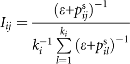

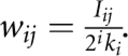4. Test each SNP using an association test. Denote p_ij^a the P- value of the association test at the jth SNP in the ith group. Then, we declared that the jth SNP in the ith group is significant at a level of α if p_ij^a≤αw_ij.

Here, k₁ is a parameter in our algorithm. We used k₁=20 in our simulation studies. However, the results are robust to the choice of k₁ as we used different weights for SNPs within each group. More discussion will be given later in the discussion section.

Statistics

We needed two test statistics. One was for the screening test used in the first stage. The other was for the association test used in the second stage. The two test statistics used in this article are those proposed by Feng et al.⁹ These test statistics can be applied to general pedigree data and can corporate the founder's phenotype. In brief, consider a sample containing n pedigrees. Suppose that the ith pedigree contains n_i informative nuclear families (with both parents and at least one being heterozygous or with at most one parent and two or more children) and the jth informative nuclear family in the ith pedigree contains n_ij children. For the jth informative nuclear family in the ith pedigree, we used (Y_ijF, Y_ijM, Y_ij1, …, Y_ijnij) and (X_ijF, X_ijM, X_ij1, …, X_ijnij) to denote trait values and genotypic scores of the parents and children. We defined the mean within-family genotypic score as if the genotypic information of both parents is available, and as

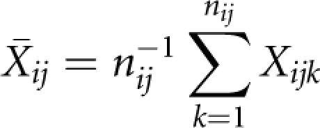if otherwise. In addition, we defined the mean within-family trait value of the children as

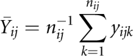and the overall mean genotypic score and trait value across the whole sample as X̄ and Ȳ. Then, the screening test statistic was given by

in which

and δ_ijF=1 (δ_ijM=1) if the father (mother) of the jth nuclear family in the ith pedigree is a founder, and =0 otherwise.

The association test proposed by Feng et al⁹ used in the second stage is the quantitative pedigree disequilibrium test.¹² The test statistic is given by

in which

Under the null hypothesis of no association, both T_screen and T_a asymptotically follow the standard normal distribution. The screening test uses the between-family and founder's information. The association test uses the within-family information and thus is robust to population stratification.

Simulation designs

We evaluated the type I error of our proposed data-driven weighting method and compared the power of the method with that of the top R and exponential weighting methods using simulation studies. We carried out simulation studies under several scenarios that included different LD structures, family structures, and population structures. Under each scenario, we simulate M=100 000 bi-allelic markers for each individual.

A homogeneous population

In a homogeneous population, the simulation studies include two types of family structures and two types of LD structures. The two types of family structures are trio structure and the CEPH family structure.^{9, 13} Each CEPH family contains three generations: four founders, two parents, and eight grandchildren (see Morley et al¹³ for more details). The two types of LD structures include (1) no LD between SNPs and (2) with LD between SNPs.

For each family structure, we generated genotypes of sampled individuals by first generating genotypes of the founders and then generating genotypes of the children by Mendelian law. For the case of no LD, we generated the founder's genotypes at each SNP by assuming that the minor allele frequency follows a uniform distribution on interval [0.1, 0.5]. For the case of with LD, we generated the founder's genotypes using the ms program by Hudson.¹⁴ In the ms program, we used a mutation rate of 2.5 × 10⁻⁸ per nucleotide per generation, a recombination rate of 10⁻⁸ per pair of nucleotides per generation, and an effective population size of 10 000. These choices were also adopted in Nordborg and Tavare,¹⁵ Kimmel and Shamir,¹⁶ and Feng et al.⁹

Under each scenario, the sample sizes are 400 trios in the trio family structure and 200 CEPH families in the extended family structure. For power comparison, we supposed that there is one disease locus. After we generated the genotypes for all sampled individuals, we randomly chose one SNP at which the minor allele frequency among founders is between 0.1 and 0.4 as the disease locus.

To evaluate type I error rates, we followed Feng et al⁹ to generate trait values under null hypothesis. For a nuclear family with m children, let Y₁=(y_F, y_M) and Y₂=(y₁, y₂,…,y_m) denote the trait values of the parents and the m children. Assume that (Y₁, Y₂) follows a multivariate normal distribution with mean vector of zero and variance–covariance matrix of

where

This covariance structure means that the father and mother are independent, and parents with children and children with children are correlated with correlation coefficient of ρ (ρ=0.2 is used in this study). The conditional distribution of Y₂=(y₁,…,y_m), given the parental trait values Y₁=(y_F, y_M), is a multivariate normal distribution with a mean vector of

and a variance–covariance matrix of

To generate trait values of all individuals in a pedigree, we first generated the trait value of each founder by using a standard normal distribution. The trait values of other members can be generated by a multivariate normal distribution with mean vector of μ_c and variance–covariance matrix of ∑_c, given the trait values of their parents.

For power comparisons, we generated trait values of a pedigree with B members from model y_b=x_bβ+ɛ_b(b=1, 2,…,B) in which x_b is the additive genotypic score at the disease locus, β is a constant, and ɛ₁,…,ɛ_B are background trait values generated under the null hypothesis using aforementioned method. The value of β is determined by heritability h and is given by

in which f is the minor allele frequency at the disease locus.

A structured population

Consider a structured population that consists of two distinct subpopulations with different allele frequencies and distinct phenotypic means. In this set of simulation studies, we considered two family structures as we did for the homogeneous population but only one LD structure, that is, no LD between SNPs. To generate genotypes of founders in a structured population, we followed Ionita-Laza et al.² For each SNP, we randomly selected a number between 0.1 and 0.9 as the ancestral population allele frequency p. Then, we independently drew two values from a beta-distribution with parameters p(1–F_st)/F_st and (1–p)(1–F_st)/F_st and scaled them to the interval (0.1, 0.9) as allele frequencies for the two subpopulations, in which F_st is Wright's measure of population subdivision.¹⁷

The phenotype under null hypothesis was generated similar to that in a homogeneous population. The only difference is that, in the structured population, we generated trait values of the founders in subpopulation 1 from the standard normal distribution and those in subpopulation 2 from a normal distribution with mean 0.2 and variance 1. As argued by Ionita-Laza et al,² the differences in allele frequencies and phenotypic means together result in spurious associations. For power comparisons, trait values are generated in the same way as that in a homogeneous population.

Results

Type I error rates

Under each of the simulation scenarios, we generated T=1000 data sets to estimate type I error rates of the three approaches. For each approach, we estimated its type I error rate as 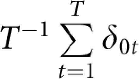in which for the tth data set δ_0t=1 if one or more markers were claimed to be significant, and =0 otherwise.

For 1000 replications, the 95% confidence interval of type I error rates is (0.036, 0.064) for a nominal level of 0.05. Tables 1 and 2 list the estimated type I error rates of the three approaches in the case of a homogeneous population and a structured population, respectively. From the two tables, we can say that, either in a homogeneous population or a structured population, almost all of the estimated type I error rates are within the 95% confidence interval, which means that the three approaches are robust to LD structure and population stratification.

Table 1. Type I error rates for the case of a homogeneous population (nominal level α=0.05).

	400 tros		200 CEPHs
	Without LD	With LD	Without LD	With LD
Data-driven weighting	0.051	0.024	0.041	0.029
Exponential weighting	0.047	0.045	0.054	0.033
Top R	0.048	0.052	0.049	0.042

In the top R method, R=20 and in the exponential weighting method, r₁=20.

Table 2. Type I error rates for the case of a structured population (nominal level α=0.05).

	400 tros			200 CEPHs
	Fst			Fst
	0.001	0.005	0.01	0.001	0.005	0.01
Data-driven weighting	0.041	0.053	0.037	0.052	0.051	0.059
Exponential weighting	0.034	0.038	0.055	0.055	0.039	0.053
Top R	0.052	0.047	0.054	0.051	0.049	0.056

In the top R method, R=20 and in the exponential weighting method, r₁=20. F_st is Wright's measure of population subdivision.

Power comparisons

For power comparisons, we simulated T=1000 data sets under each of the simulation scenarios. Each data set contains either 400 trios or 200 CEPH pedigrees. For a given approach, we assessed its power as the proportion of the simulated replications at which the method successfully identified the disease locus. Precisely, we assess the power as in which for the tth data set δ_1t=1 if the disease locus is detected, and =0 otherwise.

With parental phenotypes

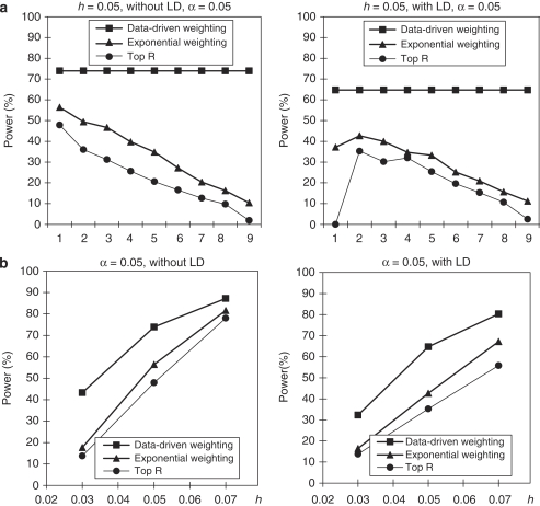
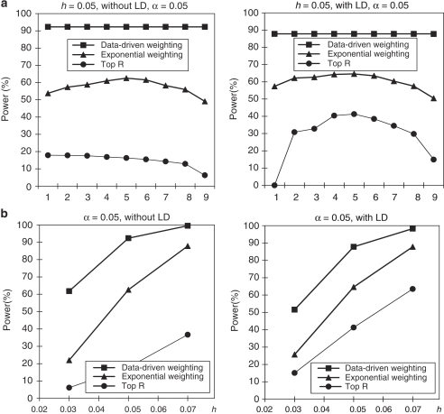
We assumeed that parental phenotypes are available. In the homogeneous population, we first considered the trio design (Figure 1). In the trio design, we compared the power of our data-driven weighting scheme with that of the top R method for different values of R and exponential weighting method for different values of r₁ (Table 3). From Figure 1a, we can see that our data-driven weighting method is consistently more powerful than the top R method and exponential weighting method, regardless of marker LD and the values of R and r₁. Figure 1b gives power comparisons of the three methods for different values of heritability and different LD structures when R and r₁ in the top R method and the exponential weighting method are chosen by their corresponding optimal values. Again, Figure 1b shows that our proposed method is consistently more powerful than the other two methods for different values of heritability and different LD structures.

Figure 1.

Power comparisons based on 400 trios in a homogeneous population with parental phenotypes. (a) The power comparisons for different values of R and r₁ in the top R and exponential weighting methods (see Table 3 for the values of R and r₁ corresponding to each scale on the x axis). (b) The power comparisons for different values of heritability h when R and r₁ in the top R and exponential weighting methods are chosen by their optimal values.

Table 3. The values of R and r₁ for each scale on the x axis.

Scale on x axis	1	2	3	4	5	6	7	8	9
R	1	5	10	20	50	100	200	500	10 000
r1	1	3	5	10	20	50	100	200	500

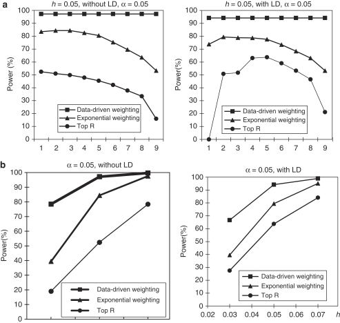
For the CEPH family structure, we used the same simulation setup as that for the trio family structure. The pattern of power comparisons for the CEPH family structure (Figure 2) is very similar to that for the trio family structure. Summarizing the results mentioned above, we may conclude that our proposed weighting scheme is more powerful than the top R method and exponential weighting method, regardless of the LD structure, family structure, and heritability.

Figure 2.

Power comparisons based on 200 CEPH families in a homogeneous population with parental phenotypes. (a) The power comparisons for different values of R and r₁ in the top R and exponential weighting methods (see Table 3 for the values of R and r₁ corresponding to each scale on the x axis). (b) The power comparisons for different values of heritability h when R and r₁ in the top R and exponential weighting methods are chosen by their optimal values.

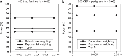
We also compared the power of the three methods in a structured population. The results of power comparisons are summarized in Figure 3. From this figure, we can make the following two conclusions. One is that our data-driven weighting method is more powerful than the other two methods for different family structures and different values of F_st (which measures the ‘how' difference of the two subpopulations). The other is that the power of all the three methods is not much affected by different values of F_st, which means that the power of the three methods is relatively robust to population stratification. Ionita-Laza et al² has pointed out that the power of the top R method will be affected by F_st if R is fixed, for example, R=10. Our results do not contradict with that of Ionita-Laza et al because our conclusion for the top R and exponential weighting methods is based on the fact that R and r₁ in the two methods are chosen by their optimal values and the optimal values depend on the value of F_st.

Figure 3.

(a) The power comparisons for 400 triad families. (b) The power comparisons for 200 CEPH pedigrees. Power comparisons for different values of F_st in a structured population with parental phenotypes. R and r₁ in the top R and exponential weighting methods are chosen by their optimal values and heritability h=0.05.

Without parental phenotypes

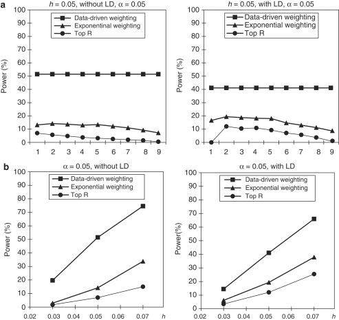
In this set of simulations, we assumed that parental phenotypes are not available. The simulation setup is the same as that in the section of ‘With Parental Phenotypes', but the minor allele frequency at each SNP (in the case of no LD) is simulated from a beta-distribution with parameters 3/14 and 1/2 (scale them to the interval (0.1, 0.5)) instead of a uniform distribution. The power comparisons in this set of simulations are summarized in Figures 4, 5 and 6. From these figures, we can see that the patterns of power comparisons without parental phenotypes are very similar to that with parental phenotypes.

Figure 4.

Power comparisons based on 400 triads in a homogeneous population without parental phenotypes. (a) The power comparisons for different values of R and r₁ in the top R and exponential weighting methods (see Table 3 for the values of R and r₁ corresponding to each scale on the x axis). (b) The power comparisons for different values of heritability h when R and r₁ in the top R and exponential weighting methods are chosen by their optimal values.

Figure 5.

Power comparisons based on 200 CEPH families in a homogeneous population without parental phenotypes. (a) The power comparisons for different values of R and r₁ in the top R and exponential weighting methods (see Table 3 for the values of R and r₁ corresponding to each scale on the x axis). (b) The power comparisons for different values of heritability h when R and r₁ in the top R and exponential weighting methods are chosen by their optimal values.

Figure 6.

(a) The power comparisons for 400 triad families. (b) The power comparisons for 200 CEPH pedigrees. Power comparisons for different values of F_st in a structured population without parental phenotypes. In both panels, R and r₁ in the top R and exponential weighting methods are chosen by their optimal values.

Discussions

In this article, we proposed a novel data-driven weighting scheme for family-based two-stage association studies. This scheme improves the exponential weighting method of Ionita-Laza et al² by allowing different weights for SNPs in the same group. Our simulation studies show that the proposed weighting scheme is consistently more powerful than the top R method with the optimal value of R and the exponential weighting scheme with the optimal value of r₁ in all the cases that we considered in the simulation studies.

The innovation of our new scheme is that it uses the between-family information to calculate marker-specific weights. In contrast, the classical top R and exponential weighting approaches only use the between-family information to rank the SNPs. Our proposed weighting scheme is not only applicable to two-stage family-based association studies, but also to other two-stage approaches as long as the statistics used in the two stages are independent or orthogonal. For example, Chung et al¹⁸ analyzed the orthogonal property between some linkage statistics and family-based association statistics. Our weighting scheme can be applied to a two-stage approach in which the first stage is a linkage test and the second stage is a family-based association test and the two tests are independent or orthogonal.

One thing to be mentioned is that when we performed the power comparison, our proposed method used a constant value for parameter k₁ (k₁=20), and the top R method and exponential weighting method used the optimal value of R and r₁, respectively. In practice, it is difficult to know the optimal values for R or r₁. The optimal value of R or r₁ depends on multiple factors, for example, pedigree structure, marker LD, heritability, and so on. The optimal value is small in the absence of LD between SNPs. In the presence of LD, the optimal value of R or r₁ could be much larger. To evaluate the effect of parameter k₁ in our proposed method, we have conducted simulation studies for k₁=1, 5, 10, 20, 50, and 100. The simulation studies (results are not shown) showed that the results of our proposed method are very similar for different values of k₁, which means that our proposed method is relatively robust to different choices of k₁.

In this study, we assumed consistent genetic effects across all ages. We realize that this assumption may not be true for some diseases, for example, childhood asthma versus adult asthma, childhood obesity versus adult obesity (see Lasky-Su et al¹⁹). For the diseases in which the genetic effects are age dependent, we may need to incorporate age of onset into association tests. However, further analysis on how to incorporate age of onset into testing is needed.

The authors declare no conflict of interest.

References

- Steen KV, McQueen MB, Herbert A, et al. Genomic screening and replication using the same dataset in family-based association testing. Nat Genet. 2005;37:683–691. doi: 10.1038/ng1582. [DOI] [PubMed] [Google Scholar]
- Ionita-Laza I, McQueen MB, Laird NM, Lange C. Genome-wide weighted hypothesis testing in family-based association studies, with an application to a 100k scan. Am J Hum Genet. 2007;81:607–614. doi: 10.1086/519748. [DOI] [PMC free article] [PubMed] [Google Scholar]
- Herbert A, Gerry NP, McQueen MB, et al. A common genetic variant is associated with adult and childhood obesity. Science. 2006;312:279–283. doi: 10.1126/science.1124779. [DOI] [PubMed] [Google Scholar]
- Spielman RS, McGinnis RE, Ewens WJ. Transmission test for linkage disequilibrium: the insulin gene region and insulin-dependent diabetes mellitus (IDDM) Am J Hum Genet. 1993;52:506–516. [PMC free article] [PubMed] [Google Scholar]
- Claton D, Jones H. Transmission/Disequilibrium test for extended marker haplotype. Am J Hum Genet. 1999;65:1161–1169. doi: 10.1086/302566. [DOI] [PMC free article] [PubMed] [Google Scholar]
- Schaid DJ, Rowland CM. Quantitative trait transmission disequilibrium test: allowance for missing parents. Genetic Epidemiol. 1999;17:S307–S312. doi: 10.1002/gepi.1370170752. [DOI] [PubMed] [Google Scholar]
- Zhao H, Zhang S, Merikangas KR, et al. Transmission/disequilibrium test using multiple tightly linked markers. Am J Hum Genet. 2000;67:936–946. doi: 10.1086/303073. [DOI] [PMC free article] [PubMed] [Google Scholar]
- Selman H, Roeder K, Devlin B. Transmission/disequilibrium test meets measured haplotype analysis: family-based association guided by evolution of haplotype. Am J Hum Genet. 2001;68:1250–1263. doi: 10.1086/320110. [DOI] [PMC free article] [PubMed] [Google Scholar]
- Feng T, Zhang S, Sha Q. Two-stage association tests for genome-wide association studies based on family data with arbitrary family structure. Eu J Hum Genet. 2007;15:169–1175. doi: 10.1038/sj.ejhg.5201902. [DOI] [PubMed] [Google Scholar]
- Rubin D, van der Laan M, Dudoit S.Multiple testing approaches which are optimal at a simple alternative Collection of Biostatistics Research Archive 2006 , http://www.bepress.com/ucbbiostat/paper 171.
- Roeder K, Devlin B, Wasserman L. Improving power in genome-wide association studies: weights tip the scale. Genet Epidemiol. 2007;31:741–747. doi: 10.1002/gepi.20237. [DOI] [PubMed] [Google Scholar]
- Zhang S, Zhang K, Li J, Sun FZ, Zhao H. Test of linkage and association for quantitative traits in general pedigree: the quantitative pedigree disequilibrium test. Genetic Epi. 2001;18 (Suppl 1:370–375. doi: 10.1002/gepi.2001.21.s1.s370. [DOI] [PubMed] [Google Scholar]
- Morley M, Molony CM, Weber T, et al. Genetic analysis of genome-wide variation in human gene expression. Nature. 2004;430:743–747. doi: 10.1038/nature02797. [DOI] [PMC free article] [PubMed] [Google Scholar]
- Hudson RR. Generating samples under a Wright-Fisher neutral model of genetic variation. Bioinformations. 2002;18:337–338. doi: 10.1093/bioinformatics/18.2.337. [DOI] [PubMed] [Google Scholar]
- Nordborg M, Tavare S. Linkage disequilibrium: what history has to tell us. Trends Genet. 2002;18:83–90. doi: 10.1016/s0168-9525(02)02557-x. [DOI] [PubMed] [Google Scholar]
- Kimmel G, Shamir R. A fast method for computing high significance disease association in large population-based studies. Am J Hum Genet. 2006;79:481–492. doi: 10.1086/507317. [DOI] [PMC free article] [PubMed] [Google Scholar]
- Balding DJ, Nichols RA. A method for quantifying differentiation between populations at multi-allelic loci and its implications for investigating identity and paternity. Genetica. 1995;96:3–12. doi: 10.1007/BF01441146. [DOI] [PubMed] [Google Scholar]
- Chung RH, Hauser ER, Martin ER. Interpretation of simultaneous linkage and family-based association tests in genome screens. Genet Epidemiol. 2007;31:134–142. doi: 10.1002/gepi.20196. [DOI] [PubMed] [Google Scholar]
- Lasky-Su J, Lyon HN, Emilsson V, et al. On the replication of genetic associations: timing can be everything! Am J Hum genet. 2008;82:849–858. doi: 10.1016/j.ajhg.2008.01.018. [DOI] [PMC free article] [PubMed] [Google Scholar]