

Abstract
Motivation: Exploitation of locally similar 3D patterns of physicochemical properties on the surface of a protein for detection of binding sites that may lack sequence and global structural conservation.
Results: An algorithm, ProBiS is described that detects structurally similar sites on protein surfaces by local surface structure alignment. It compares the query protein to members of a database of protein 3D structures and detects with sub-residue precision, structurally similar sites as patterns of physicochemical properties on the protein surface. Using an efficient maximum clique algorithm, the program identifies proteins that share local structural similarities with the query protein and generates structure-based alignments of these proteins with the query. Structural similarity scores are calculated for the query protein's surface residues, and are expressed as different colors on the query protein surface. The algorithm has been used successfully for the detection of protein–protein, protein–small ligand and protein–DNA binding sites.
Availability: The software is available, as a web tool, free of charge for academic users at http://probis.cmm.ki.si
Contact: dusa@cmm.ki.si
Supplementary information: Supplementary data are available at Bioinformatics online.
1 INTRODUCTION
In the Protein Data Bank (PDB), there are presently 8000 protein structures derived from structural genomic studies and 2000 of these have no known function (Berman et al., 2002). Binding sites are closely related to protein function, the identification of binding sites in proteins is essential to an understanding of their interactions with ligands, including other proteins. Many computational tools for the analysis (Tuncbag et al., 2009) and prediction (Ezkurdia et al., 2009) of binding sites have been reported.
Binding sites can retain conservation of sequence and structure (Keskin et al., 2005; Valdar and Thornton, 2001). Structural conservation however is more prevalent (Lecomte et al., 2005). Even in the absence of obvious sequence similarity, structural similarity between two protein structures can imply common ancestry, which in turn can suggest a similar function (i.e. a binding site). However, it is also possible for structurally similar proteins to have different functions, and similar folding by itself does not necessarily imply evolutionary divergence (Russell et al., 1997). In the case of divergent evolution, similarity is due to the common origin, such as accumulation of differences from homologous ancestral protein structures. In contrast, convergent evolution arises as a result of some sort of ecological or physical drivers toward a similar solution, even though the structure has arisen independently. A rough estimate is that the frequency of two different folds converging to a similar statistically significant side-chain pattern is ∼1% (Russell, 1998). It has been shown that convergent evolution of enzyme binding sites is not a rare phenomenon (Gherardini et al., 2007).
If a protein has no known function, but a known 3D structure, inferences concerning function can be made by comparison to other proteins. Recently, a number of web servers for local structural alignment have become available. These provide comparison of pre-selected parts of proteins (e.g. binding sites, user-defined structural motifs) (Angaran et al., 2009; Debret et al., 2009; Shulman-Peleg et al., 2008) against binding sites or whole-protein structural databases. The MultiBind and MAPPIS servers (Shulman-Peleg et al., 2007, 2008) allow the identification of common spatial arrangements of physicochemical properties such as H-bond donor, acceptor, aliphatic, aromatic or hydrophobic in a set of user provided protein binding sites defined by interactions with small molecules (MultiBind) or in a set of user-provided protein–protein interfaces (MAPPIS). Others provide comparison of entire protein structures (Ausiello et al., 2008) against a number of user submitted structures. Unlike global alignment approaches, local structural alignment approaches are suited to detection of locally conserved patterns of functional groups, which often appear in binding sites and have significant involvement in ligand binding (Shulman-Peleg et al., 2007).
In this article, we describe an algorithm ProBiS, which, in contrast to these methods, enables local structural alignment of entire protein surface structure against a large database of protein structures in reasonable time. It detects structurally similar regions in a query protein by mapping structural similarity scores on its surface. The comparison involves geometry and physicochemical properties, and is conducted at the level of amino acid functional groups. For each pairwise comparison of the query protein to a database protein, the algorithm produces multiple local alignments of the surface regions that are found in both; no attempt is made to align the proteins globally and similar folding is not a requirement for a relationship between the two proteins. Since no presumptions about localization of binding sites prior to comparison are used, ProBiS may detect new binding sites and suggest ligands that these binding sites may accommodate.
ProBiS is a generalization of our earlier algorithm that predicts protein–protein binding sites by searching for conserved protein surface structure and physicochemical properties in proteins with similar folds, and permitting comparison of only a few structural neighbors (Carl et al., 2008; Konc and Janežič, 2007a). Major extensions of the ProBiS algorithm over the earlier algorithm include:
Comparison of proteins regardless of their fold similarities. ProBiS compares the query protein with a database of over 23 000 protein structures. In contrast to the previous algorithm, which simultaneously compares only a few proteins with similar folds, ProBiS identifies all proteins that share local similarities with the query protein. It then calculates local structural similarity scores of query protein residues in each of these retrieved proteins and in this way detects structurally similar regions, which often correspond with binding sites.
Detection of similarities between backbone segments with different conformations (e.g. flexible loops) in the query and database proteins. Such similar backbone segments are detected by 3D comparison of protein backbones.
Assignment of a number of different scores to every structural alignment. These scores are designed to measure statistical and structural significance and are the basis for the retrieval of similar proteins from the database; only alignments with favorable scores are retained for further analysis of structural similarity.
Detection of ‘fingerprints’ that are highly conserved amino acid residues within the most reliable local structural alignments found. These are most commonly of proteins with the same fold as the query protein. The remaining structural alignments are subsequently examined for similar motifs. As a result, proteins that share with the query protein a structurally similar binding site but have a different fold can be retrieved from the protein database.
Storage of results in a database, each entry of which has a record of the aligned residues, rotational matrix, translational vector and alignment scores.
The advantages and limitations of ProBiS in the detection of protein–protein, protein–small ligand and protein–DNA binding sites are described using a quantitative performance evaluation on a test set of 39 proteins. The results show that ProBiS outperforms other methods that rank amino acid residues by degree of sequence conservation and also energy-based methods. Unlike global structural alignment approaches, ProBiS yields high-quality local structural alignments of proteins with dissimilar folds, and aligns similar binding sites without presumption of their whereabouts in the compared structures. The extent of structural similarity in protein–protein and protein–small ligand binding sites is also discussed.
2 METHODS
ProBiS detects surface structural patches that are common to the query protein and a database protein. The algorithm identifies structurally similar sites, whose constituent residues may be scattered in sequence, but are close together in structure. Such similar patches are often related to ligand binding and the search for them exploits the fact that binding sites share similar patterns of interactions in proteins which perform similar functions but may or may not have different folding patterns. The possible interactions are represented with sub-residue precision and a structural similarity search algorithm, which employs a fast maximum clique algorithm and operates independently of fold and sequence, performs a local, surface-oriented comparison of the proteins.
A clique is a subset S of vertices in a graph, composed of vertices and edges, such that each pair of vertices in S is connected by an edge. A maximum clique in a given graph is the clique with the largest number of vertices. The maximal clique algorithm of Bron and Kerbosch, which has previously been used to compare binding sites (Schmitt et al., 2002), significantly differs from our maximum clique algorithm (Konc and Janežič, 2007b). While a maximal search is for all cliques that are not subgraphs of any other clique, maximum clique algorithms search only for the clique with the maximum number of vertices. Consequently, although both address a NP-hard problem, finding a maximum clique requires an order of magnitude less computation time.
Using a fast maximum clique algorithm and a strategy of dividing graphs into subgraphs, enables our approach to the comparison of complete protein surfaces. ProBiS compares the query protein structure sequentially to proteins in the PDB and retrieves structures that share local structural similarities with the query protein. It uses these similar structures to generate a structure-based sequence alignment of the query protein with the proteins from the database and then calculates the similarity score for each query protein surface residue, projecting these scores as colors onto the surface of the query protein. Each of these steps is described in detail in the following sections.
2.1 Representation of protein surfaces
Residues on the protein surface are identified by an algorithm that identifies the solvent accessible surface atoms (Konc et al., 2006). This subset of all the protein atoms is represented as a series of graphs of vertices and edges, as shown in Figure 1. Vertices are points in 3D space, and each replaces one functional group belonging to a residue on the protein surface.
Fig. 1.

Different functional groups in proteins are assigned distinct labels (see color encoding). Subgraphs are generated from the query protein and each database protein and then used to produce product graphs which reveal the extent of superposition of any pair of subgraphs.
Functional groups are specific groups of atoms within these residues responsible for the characteristic interactions of the protein with other molecules. Each vertex is labeled with the physicochemical properties of a functional group that it replaces, hydrogen bond acceptor (AC), hydrogen bond donor (DO), mixed acceptor/donor (ACDO), aromatic (PI) and aliphatic (AL); (Schmitt et al., 2002).
To compare two proteins, represented as graphs, a product graph is constructed as shown in Figure 1. The corresponding vertices in this product graph are pairs of vertices with identical physicochemical properties (u1, u2), e.g. two acceptors: (AC, AC), and each of the two vertices in the pair is derived from its own protein graph. Two vertices (u1, u2) and (v1, v2) of a product graph are connected by an edge if and only if distances between u1 and v1 and between u2 and v2 differ by <2 Å (Konc and Janežič, 2007a). Protein graphs can be regarded as rigid 3D protein structures of vertices, and a product graph constructed from two such graphs is an approximate representation of all possible rotations and translations of one protein graph onto the other. A maximum clique in the product graph corresponds to the rotational–translational variation that superimposes on, or aligns with the largest number of vertices in the two protein graphs.
2.2 The ProBiS algorithm
A local structurally similar site is defined as one or more surface functional groups that adopt a similar geometrical arrangement in two or more compared proteins. The vertices representing these groups can be superimposed with a low root mean square deviation (RMSD), but such a local alignment does not guarantee that entire protein backbones can be superimposed. Protein surface residues are represented as vertices in 3D space and a structurally similar site is merely one with a similar geometrical arrangement of vertices. A maximum clique in the product graph described above is equivalent to a vertex similarity between the two proteins, and in turn, each such vertex similarity, is equivalent to a local structural alignment of common surface residues. A crucial step in the comparison of whole-protein surfaces is the division of protein graphs into subgraphs and filtering of these that precedes the actual comparison using the computationally intensive maximum clique algorithm. The strategy of the ProBiS algorithm is presented schematically in Figure 2. The method, steps A–E corresponding to those in Figure 2, is described in greater detail as follows.
Fig. 2.

Schematic representation of the ProBiS algorithm. (A) The query protein structure (Q) is compared in a pairwise manner with each of ∼23 000 non-redundant structures (P). (B) Proteins, represented as graphs of vertices (white dots) and edges (not shown), are divided into n overlapping subgraphs, where n equals the number of vertices and all vertices are within 15 Å of a central vertex: three subgraphs per protein are depicted here as distinctly colored encirclements. A fast distance-matrix-based filtering is applied to them to eliminate non-similar subgraphs. (C) A product graph is constructed for each similar pair of subgraphs (see color encoding in B and C). A maximum clique (thick lines) in a product graph represents the largest similarity between two compared protein subgraphs. (D) Each maximum clique produces a structural alignment of two compared proteins (the alignment shown corresponds to the middle maximum clique in C). (E) Steps A–D are repeated for each protein from the nr-PDB and the results are stored in a MySQL database. Structural similarity scores are calculated and projected on the query protein surface. Structurally similar and variable residues are colored red and blue, respectively. High-scoring residues are considered as predicted structurally similar binding sites.
(A) A query protein structure (Q) whose structurally similar regions are to be detected is compared with each of ∼23 000 non-redundant PDB structures (P). Residues on the surface of the proteins, identified by a solvent accessible surface algorithm (Konc et al., 2006), are represented as graphs with vertices and edges, and their functional groups are replaced by one of the five vertex types which are shown as white dots in Figure 2B. Finally, vertices that are separated by<15 Å are connected with edges.
(B) Proteins represented as graphs of vertices and edges, are divided into n overlapping subgraphs, where n is the number of vertices in each protein graph. Figure 2B shows two proteins, with three such subgraphs for each protein depicted as distinctly colored regions. A subgraph of a protein graph is defined as all vertices within 15 Å of a central vertex, and is compactly represented as a distance matrix of these neighboring vertices. To find if two such subgraphs, i.e. two distance matrices, represent similar parts of their respective protein surfaces, the two distance matrices are subtracted, and from the resulting difference matrix, a value of similarity is calculated (as described in Konc and Janežič, 2007a). For each pair of query and database protein's subgraphs, which are similar as judged by this value, a product graph is constructed. This ensures that only pairs of subgraphs that have sufficiently similar geometrical arrangements of vertices and with similar physicochemical properties proceed to the next, computationally intensive step.
(C) All sufficiently similar pairs of subgraphs that pass the filtering in the previous step are then subjected to the more rigorous maximum clique procedure, which detects vertex-to-vertex correspondences between the two protein graphs being compared. A product graph is constructed for each such pair of protein subgraphs as described above. The algorithm then finds a maximum clique in each product graph by examining approximately 100–1000 product graphs with up to 1000 vertices each in each protein–protein comparison. A maximum clique in a product graph corresponds to a largest common vertex substructure, which can be translated to a maximum substructure common to the two compared proteins. Maximum cliques of 3, 4 and 3 vertices are shown as thick lines in Figure 2C.
(D) Each maximum clique is equivalent to a single structural alignment and superimposition of two compared proteins. The alignments are local, and allow superimposition of maximum numbers of two protein subgraph vertices. Alignment scores such as surface vectors angle, RMSD and expectation values (E-values) are calculated for each such local superimposition of the two proteins, as discussed in Section 2.4, subsequently. These alignment scores measure the statistical and structural significance of the different local structural superimpositions and allow filtering out of insignificant structural alignments. Maximum cliques passing this filter and possessing at least five common vertices are joined into clusters, which represent the larger structural similarities in the protein surfaces being compared. Finally, a search for similarities in flexible parts of the two compared proteins is conducted, as described below.
(E) Steps A–D are repeated for each database protein and the resulting alignments and their scores are saved to a results database implemented on the MySQL platform. The significant local structural alignments can be retrieved from this results database, using the alignment scores as search parameters. Only local structural alignments with favorable scores (Section 2.4) are considered further in the calculation of similarity scores. For every surface residue in the query protein, ProBiS first sums the number of times it is found in all favorable local structural alignments. These sums, one for each residue, are then translated into discrete similarity scores ranging from 0 (blue) to 9 (red) and the appropriate colors are applied to the structure of the query protein. To facilitate the comparison with other methods, all query protein surface residues with structural similarity scores of 7, 8 or 9 are arbitrarily considered to be parts of binding sites.
2.3 Protein flexibility
Many proteins are flexible, capable of adopting different conformations and an algorithm that detects similarities in purely rigid structures will have only limited value. This problem is addressed by searching for backbone segments with residue compositions and orientations that are similar in the query protein and the database protein, but which may adopt different conformations in the two proteins. Each maximum clique, i.e. its rotational–translational variation, representing a rigid, local similarity, is used to locally superimpose the two compared protein structures and then their backbones are examined for pairs of three consecutive amino acid residues meeting the following conditions.
The distance between the two Cα atoms of the two middle residues must be <10 Å.
The amino acid codes of three residues of the first protein, must be similar to those of the second protein. A BLOSUM62 (Blocks Substitution Matrix) matrix is used to score the match of each residue pair in these three residue-long alignments (Henikoff and Henikoff, 1992). To exclude spurious matches composed solely of hydrophobic residues, the cumulative score for the three residues must be >12.
For each of the three similar residues in a pair of proteins a vector between the first and the third Cα atom is drawn. To ensure similarly oriented matches, the angle between two such vectors must be <45○.
Once identified, these backbone segments of three residues are extended in both directions by adding a new residue to both ends. This is done independently of sequence order. A pair of residues is only added if it lowers the expectation value (see Section 2.4, subsequently) of the alignment. No gaps are allowed and the distances between pairs of newly added residues may be >10 Å.
2.4 Local structural alignment scores
A number of scores are used to measure the statistical and structural significance of the local structural alignments and to permit filtering out of insignificant alignments (see Section 2.2, step D). Since local structural alignments need not involve a large number of residues, the similarity that is detected could in fact be a frequently occurring 3D motif, having no relationship to common protein function. Further, surface properties in the two aligned surface regions may differ, e.g. the surfaces may have different curvatures, or they may be differently oriented. The first step in the calculation of scores is the local superimposition of the two compared proteins, based on the rotational and translational variation imposed by a maximum clique. Then, four distinct criteria are applied to each such local structural alignment.
Surface vectors angle: for each of the two superimposed sets of vertices, an outer-pointing surface vector originating in the geometric center and perpendicular to the surface of the protein is constructed. These vectors each represent the orientation of one of the two superimposed surface patches of vertices and a smaller angle between them indicates a similar orientation of the surfaces in this region. Local structural alignments with surface vector angles <90○ are retained.
Surface patch RMSD: calculated for each pair of superimposed vertices, this measures the shape similarity of the two superimposed surface patches. Local structural alignments having surface patch RMSD <2.0 Å are accepted.
Surface patch size: structural alignments with fewer than 10 vertices are discarded.
E-value: ProBiS algorithm calculates an E-value for each local structural alignment using the Karlin–Altschul equation (Altschul and Gish, 1996; Altschul et al., 1997; Karlin and Altschul, 1990). More details are given in the Supplementary Material. In this calculation, vertices in the structural alignment are converted back to the corresponding residues and each residue may be represented by more than one vertex. Consequently, only one occurrence of each residue in the alignment is counted. In contrast to sequence alignment approaches, gap penalties are not included in the calculation of E-values, since structurally similar residues on a protein surface may by definition, be quite separate in the protein sequence. The lower the E-value, the less likely that the match is by chance, and the greater significance of the local structural alignment. The threshold E-value for acceptance of a structural alignment used here is <1 × 10⁻⁴.
The alignment scores used here have been defined by varying them systematically and observing the effects of the changes on the binding site detection.
2.5 Fingerprint residues
Residues that are important for binding of ligands need not be contiguous but are typically found in well-defined local 3D arrangements and can be regarded as a fingerprint of the specific binding site. A motif of fingerprint residues is therefore first identified in a subset of the most reliable structural alignments and then a search for a similar motif of residues is conducted among the remaining aligned proteins.
A structure-based sequence alignment of proteins with favorable alignment scores (described in Section 2.4) is constructed in which the structurally aligned protein sequences are listed in the order of their decreasing alignment lengths. Alignment length is the sum of residues in all local structural alignments that were found for a pair of compared proteins. In the second step, fingerprint residues are identified in the structure-based sequence alignment as follows.
Only proteins that structurally align to more than one-third of the query protein residues and thus represent the most trusted part of the structure-based sequence alignment are considered.
Discrete similarity scores (between 0 and 9) are calculated for this ‘most trusted’ part of the structure-based sequence alignment.
Structurally similar residues with the highest similarity score, 9 are labeled as fingerprint residues.
After the fingerprint residues have been identified, their appearance in the remainder of structurally aligned proteins is sought and protein structures that share a locally similar interaction pattern with the query protein are retrieved from the structure-based sequence alignment. For the results to be accepted, each aligned protein must have a minimum of five such fingerprint residues.
2.6 Identification of non-redundant PDB structures
A list of more than 23 000 non-redundant single chain protein structures, automatically updated each week, is prepared as follows (Figure 3): the RCSB website provides a list of clustered PDBs derived from the ∼60 000 protein structures in the PDB, in which sequences that are ≥95% identical are clustered together. The structure with the highest resolution is selected from each cluster, X-ray crystallographic structures being given preference over NMR structures. The graph representation of all selected protein structures and residues on the surface of the proteins are calculated, and are saved into ‘surface files’. These surface files represent a current view of the non-redundant database (nr-PDB), which is updated every week following the regular RCSB protein database update. Surface, instead of PDB files are used with ProBiS, since they enable faster pairwise comparisons.
Fig. 3.

Schematic representation of nr-PDB database preparation, conversion to a surface representation and ProBiS results database (MySQL).
2.7 Test set protein structures preparation
As a test set for the detection of binding sites, we use 39 non-redundant protein structures, each involved in well characterized protein–protein interactions and crystallized as a complex involving at least one other protein. The non-redundancy of the test set is achieved with the blastclust algorithm (Altschul et al., 1997), so that no two proteins (with the exception of two pairs, see Supplementary Material) have a sequence identity of >30% in a pairwise alignment covering >90% of each of their sequences. Most of these proteins also bind other ligands, such as cofactors and metal ions, which often are missing from the PDB records. Accordingly, we also identified binding sites for these ligands. A residue is part of a binding site if the distance between any of its atoms and an atom from another molecule (e.g. protein, small molecule, DNA) is less than the sum of their van der Waals radii plus 3.0 Å. Alternatively, if no ligands are available in the crystal structures, known binding site residues obtained from the catalytic site atlas (Porter et al., 2004) and literature were used. A detailed description of the identification of the missing binding sites for each of the 39 proteins can be found in the Supplementary Material.
3 RESULTS
ProBiS detects structurally similar regions and maps them on the surface of the appropriate protein structures. This is accomplished through the detection of high quality local structural alignments in a database of non-redundant protein structures. The program's performance in detecting different types of binding sites, e.g. protein–small ligand, protein–protein, protein–DNA, has been studied on a set of 39 protein structures, details of which are provided in Supplementary Material.
The local structural similarity scores generated by ProBiS are effective predictors of protein binding sites. The predictions, based solely on local structural similarity, are more accurate than those produced by ConSurf (Glaser et al., 2003, 2005), a protein surface mapping tool which depends upon sequence conservation and which to our knowledge, is the only available tool that maps sequence conservation to protein structure. ProBiS is also compared with Q-SiteFinder (Laurie and Jackson, 2005), a method which detects energetic features in protein structures favorable for ligand binding and has been benchmarked as a small-ligand as well as protein–protein binding sites detection tool (Burgoyne and Jackson, 2006). A detailed discussion of the results obtained by ProBiS is provided in the case of biotin carboxylase and in the case of TATA-binding protein (TBP); the unique ability of ProBiS to detect and align similar binding sites in protein structures with different folds and to compare it with other global and local structural alignment methods is described.
All experiments described here were performed on a 16 threaded, 8 core, 2 processor personal computer. On this computer, pairwise local alignment of two protein structures with ProBiS requires typically <1 s and running ProBiS jobs in parallel, the nr-PDB search with a query protein of ∼200 residues, involving fast filtering followed by structural similarity mapping takes ∼10 min.
3.1 Binding sites detection
A test set was prepared of 39 proteins that interact either with other proteins, or with small molecules, substrates or cofactors. In cases where the ligands were missing from the PDB files, the relevant data were supplied from the literature or from homologous cases. As described in the Supplementary Material, we considered the various different types of binding sites as a single united binding region important for protein function and we also considered each binding site type separately. Each of the 39 proteins in the test set was a query used in a search of the database of currently ca. 23 000 non-redundant protein structures extracted from the PDB. The quality of the detected binding regions was measured in terms of the specificity, sensitivity and significance of prediction, as defined below.
Specificity indicates the proportion of the residues predicted to be in the binding site which are actually in the binding site. If T residues are predicted to be in the binding site, but only S are correctly predicted, then the specificity is defined as: SP = S/T
Sensitivity is the proportion of the interface that was predicted. If the interface requires U residues but only W were correctly predicted to be in the interface, then sensitivity is defined as: SE = W/U
Significance of prediction is the probability P of randomly choosing a patch of residues equal in size to the predicted patch, but with equal or better correspondence with the actual binding site than the predicted patch (Carl et al., 2008). P is defined as:
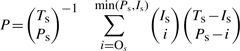 |
where Ts is the total number of protein residues, Is is the number of residues in the actual protein binding site, Ps is the number of residues in the predicted protein binding site and Os is the number of predicted residues that overlap with the actual protein binding site. For example, the value P = 0.5 for a patch of predicted residues indicates that in 5 out of 10 attempts, a patch with the same number of randomly chosen residues will lead to a better prediction of the actual binding site.
The detailed results from the 39 test set structures are presented in the Supplementary Material. The ability of ProBiS to detect protein binding regions in the test set protein structures is compared to that of ConSurf and to that of Q-SiteFinder in Table 1. ProBiS produces discrete similarity scores (0–9) and ConSurf produces conservation scores (1–9) for surface protein residues, and it is possible to compare the two methods directly. Residues with similarity scores 7–9 (ProBiS) and with conservation scores 8–9 (ConSurf), are regarded as reliable binding site predictions. Using this definition, the two methods detect almost equal number of structurally similar (ProBiS) and conserved (ConSurf) residues for a test set protein. ProBiS retrieves 62.8 structurally similar residues/protein and ConSurf retrieves 60.6 sequence conserved residues/protein (Table 1). The specificity, sensitivity and significance of prediction established by the two methods are directly comparable. The top four predicted sites proposed by Q-SiteFinder as the putative binding site are considered; a minimum of P-value at this setting is observed (Supplementary Material).
Table 1.
Binding sites detection with a structural similarity mapping method, evolutionary conservation mapping method and an energy-based method on a set of 39 proteins
| Method | Total no. of residues | Interface no. residues | No. of predicted residues | P-value (× 10−3) | SP (%) | SE (%) |
|---|---|---|---|---|---|---|
| ProBiSa | 224 | 54 | 62.8 | 1.4 | 39.0 | 43.9 |
| ConSurfb | 224 | 54 | 60.6 | 33.0 | 34.3 | 38.1 |
| Q-SiteFinder | 224 | 54 | 48.5 | 6.5 | 39.4 | 38.2 |
Tables with detailed results are available in the Supplementary Material.
aThe alignment scores listed in the ‘Methods’ section were used.
bConSurf uses different methods to count conserved residues. We used the Bayesian method which is enabled by default and gives the best results.
It can be seen from Table 1 that ProBiS achieves on average 4.7% higher specificity and 5.8% higher sensitivity than ConSurf. The lower median value, 1.4 × 10⁻³ for the significance of prediction also favors the ProBiS algorithm. While ConSurf calculates conservation scores on the basis of multiple sequence alignment typically of hundreds of homologous protein sequences, ProBiS usually uses tens of locally similar structures. These results suggest that local structural similarity provides some additional precision to the detection of binding sites. ProBiS outperforms the energy-based Q-SiteFinder method, which produces median P-value of 6.5 × 10⁻³ at a similar specificity as our algorithm and at 5.7% lower sensitivity. Consequently, structural comparison should be a method of choice in the case when 3D structural data for a protein of interest is available and there are similar structures in the PDB.
3.2 Structural similarity in protein–protein and protein–small ligand binding sites
The final test set of 39 proteins includes 39 protein–protein binding sites, 17 sites in which small ligands bind, 1 protein–DNA binding site and 1 loop, associated with protein folding. In the 39 proteins, the average protein–protein binding site contains 42.8 amino acid residues and a small-ligand binding site, 27.9 amino acid residues. Every residue involved in binding, to all ligands including cofactors and metal ions is counted in these numbers. Small-ligand binding sites have 76.0% of their residues structurally similar. In comparison, protein–protein binding sites, with the sensitivity of 38.0%, are two times less structurally similar. The only protein–DNA binding site studied (PDB: 1ytf) was predicted with the sensitivity of 63.0%, which, despite its larger size (46 residues), suggests some similarities in terms of its structural similarity scores, to the small-ligand binding sites. The sensitivities in the two major binding site classes are markedly different. However, the absolute number of structurally similar residues, calculated as the product of the average number of residues in a binding site class and the sensitivity of this class, differ less. Small ligand binding sites have, on average, 21.2, and protein–protein binding sites, 16.3 structurally similar residues. The absolute similarity as judged by structural similarity scores seems to be only moderately lower for protein–protein compared to small-ligand binding sites.
Clearly, structural similarity does not extend to entire protein–protein binding sites and cannot be used as the only predictor of a protein–protein binding site. Instead, it could be used to detect structurally conserved ‘hot-spots’ (Keskin et al., 2005), residues within protein–protein binding sites, with a particularly important function, for example, hydrogen bonding in ligand binding. Hot spots contribute the most to the binding free energy of a protein–protein complex, and their conservation in homologous sequences has been used to aid in their identification (Guney et al., 2008).
Protein–protein binding sites are mostly conserved in structural homologues while similar small-ligand binding sites are, in addition, found in structurally distant proteins that frequently adopt different folds. As an example, the P-loop, which is a small ligand binding site responsible for phosphate binding in the alpha subunit of a G-protein (PDB: 1got) is detected as structurally similar across many hundreds of database proteins, including those with different folds, while the protein–protein binding site for the beta subunit, is conserved substantially in only the nine most similar structural homologues retrieved. This is generally observed in the proteins studied and supports a hypothesis that protein–protein binding sites evolve more rapidly than protein–small ligand binding sites. Arguably, this difference may be attributed to their different biological roles: small ligands binding sites govern processes of molecular transformation, which are relatively unchanged in time, while protein–protein binding sites regulate evolutionary transient processes in which connections with different proteins are developed.
3.3 Detailed binding sites detection examples
Biotin carboxylase (PDB: 1bnc) is a homodimer with two binding sites: an active site in which the ligand biotin is bound and a binding site for the second identical protein subunit (Fig. 4A and B). A search of the nr-PDB database with one of the homodimer subunits as the query protein, resulted in 178 structures with locally similar surface patches retrieved from the nr-PDB; 79% of the active site pocket and 31% of the protein–protein binding site were found to be structurally similar. In biotin carboxylase, the two binding sites are ∼12 Å apart and conservation of one is unlikely to be correlated with that of the other. Notably, the protein–protein interface in this homodimer was found in another study (Caffrey et al., 2004) which used multiple sequence alignment of this protein's sequence homologues to determine the extent of conservation of its surface residues, to be less conserved than the rest of the exposed surface. In contrast, local structural similarity, used by ProBiS seems to be a good predictor of the protein–protein binding site, especially of residues that are involved in hydrogen bonding between the two subunits.
Fig. 4.

Structural similarity pattern in the homodimer protein biotin carboxylase (PDB: 1bnc) and in the TATA-binding protein (TBP) (PDB: 1ytf). The proteins are represented as pink cartoon models, TATA box DNA as cyan cartoon model; the structurally similar residues are shown as yellow, orange and red stick models and the interacting residues on the opposing chains are shown as pink stick models. Hydrogen bond pattern occurring (A) between biotin carboxylase and bound ligands, biotin, ADP, Mg2+ and bicarbonate ion; (B) between the two subunits of biotin carboxylase; (C) between the TBP and the transcription factor IIA and (D) between the TBP and the TATA box DNA is shown.
TATA-binding protein (TBP) recognizes a characteristic sequence of nucleotides composed of deoxyadenosine and deoxythymidine (the TATA box) and binds to it, thus marking the starting point of transcription. TBP (PDB: 1ytf) forms a complex with the transcription factor IIA (Fig. 4C) and the TATA box (Fig. 4D). Structurally similar residues in the DNA binding region of TBP form multiple hydrogen bonds with the TATA box (Fig. 4D); this region has been observed previously to be conserved in sequence (Patikoglou et al., 1999). ProBiS also identifies protein–protein binding site residues (Fig. 4C) with the sensitivity of 50% (ConSurf with the sensitivity of 16.7%). To our knowledge, the structural similarity involving these residues has not been reported previously.
3.4 Detection of similar function in structurally unrelated proteins
In order to demonstrate the unique ability of ProBiS to detect and align similar binding sites in the absence of fold similarity, we examined 10 pairs of protein structures, where the two members of a pair adopt different folds, but have a similar binding site and perform a similar function (Russell, 1998). These pairs of proteins were identified by an all-against-all comparison of SCOP (Structural Classification of Proteins) representatives and the similar binding site residues identified in each protein pair can be superimposed with low RMSD.
We performed pairwise comparisons using the ProBiS algorithm between the proteins in each pair reporting the highest scoring local structural alignment, i.e. that with the lowest E-value. Then, we compared the alignments produced by ProBiS with those of the global and local structural alignment algorithms and obtained the results shown in Table 2. All three structural alignment programs that we used for comparison, DaliLite (Holm et al., 2008), MolLoc (Angaran et al., 2009) and MultiBind (Shulman-Peleg et al., 2008), which represent different approaches to structural alignment are available as web-servers. Global alignment algorithms such as that in DaliLite maximize the aligned length and, concurrently, minimize the RMSD between two protein backbones. Local structural alignment algorithms, such as that in MolLoc and that in MultiBind, minimize the RMSD between preselected regions of the proteins, e.g. binding sites.
Table 2.
Comparison of structural alignments quality of similar binding sites on 10 protein pairs with dissimilar folds
| First protein structure |
Second protein structure |
ProBiS |
DaliLite |
MolLoca |
MultiBindb |
||||
|---|---|---|---|---|---|---|---|---|---|
| PDB | Residue numbers | Ligand | PDB | Residue numbers | Ligand | RMSDs (Å) | |||
| 1addA | 262,295,181,15,214,238 | ZN | 1bmcA | 168,90,152,86,88,149 | ZN | 6.53 | 14.31 | 13.29 | 14.59 |
| 1eceA | 114,162,238,116,161,27 | BGC | 2dnjA | 212,39,134,252,7,170 | DNA | 9.91 | 12.91 | 12.48 | 8.05 |
| 1phrA | 12,129,18,19 | SO4 | 1vhrA | 124,92,130,131 | EPE | 1.50 | 8.94 | 8.10 | 5.37 |
| 1bmfA | 269,270,273,175,176 | ANP | 1aylA | 268,269,213,254,255 | ATP | 2.34 | n/a | 3.26 | 11.93 |
| 1ampA | 179,117,256,97,228 | ZN | 1alkA | 51,327,331,370,102 | ZN | 2.14 | 10.69 | 6.60 | 11.91 |
| 1ribA | 84,237,238,118,121,122 | FEO | 1vhhA | 130,148,127,135,139,142 | ZN | 4.82 | n/a | n/a | 13.19 |
| 1powA | 308,311,286 | FAD | 1inpA | 311,370,358 | n/a | 1.07 | 35.70 | 19.75 | n/a |
| 1alkA | 369,327,101,331,370,166 | ZN | 1fjmA | 64,92,208,125,173,221 | MN | 7.00 | n/a | 9.63 | 7.92 |
| 1qbaA | 844,845,847,850,849,852 | n/a | 1eurA | 176,177,179,182,181,184 | n/a | 0.27 | 46.12 | 0.30 | n/a |
| 2kauC | 134,136,219,246,320,364 | NI | 2mhrA | 54,25,106,77,73,62 | FEO | 12.68 | 25.95 | 12.41 | 12.62 |
| Mean RMSDs (Å) | 4.82 | 22.09 | 9.54 | 10.69 | |||||
aGeometry+atom type method is used; in the two cases, where ligands are not available (n/a), we restricted the comparison to the corresponding residue numbers given above.
bThe compared binding sites are defined by the surface region within 8.0 Å from small ligands with codes ZN, MN, SO4, EPE, NI and FEO; the default threshold of 4.0 Å is used elsewhere.
The comparison between the methods listed in Table 2 is made by calculating, after superimposition, the RMSD between the similar binding site residues, which had been previously identified (Russell, 1998). DaliLite produces the worst RMSD, 22.1 Å, presumably because the protein structures that are compared do not have similar folds and consequently global alignment fails to superimpose the binding site residues. For three of the protein pairs that were examined, DaliLite does not produce any result, probably because the proteins folds are too dissimilar. In the remaining five cases, DaliLite misaligns the binding sites. MolLoc and MultiBind produce better alignments with RMSDs of 9.5 Å and 10.7 Å, respectively, but unlike ProBiS and DaliLite, do not support unsupervised comparison. Thus the user has to manually select regions of protein surfaces that are to be compared. Where the ligands are missing in the compared structures, MolLoc allows the compared binding sites to be defined with a set of user provided residues; we used residues given in Table 2. MultiBind only allows comparisons, where a ligand is present in each of the two compared binding sites, consequently for two pairs we could not perform the alignment; in all other cases, the RMSD of the alignment in the top scoring solution is presented.
In proteins which have different folds, ProBiS produces better alignments of the residues in the similar binding site detected by Russell et al. (1998) than either DaliLite, MolLoc or MultiBind to judge from the calculated RMSD between these residues. In addition, ProBiS can align protein structures in an unsupervised fashion, which allows it to perform database searches.
4 CONCLUSION
It is well known that protein binding sites are structurally similar and many methods exist that can structurally align proteins. We introduce a new approach for the detection of binding sites in a 3D protein structure by searching for the locally similar surface structures in a large database of protein structures. The maximum clique technique, the core of the algorithm detects 3D correspondences between proteins at a sub-residue level. Local structural similarity scores are calculated and mapped to the query protein surface. Such prediction of binding sites which depends on structural similarity of protein surfaces is useful and accurate and can enjoy success in structures with dissimilar folding patterns. Structural similarity can provide additional advantages over sequence conservation in the detection of functional regions such as binding sites and it is concluded that structural comparison should be the method of choice when a crystallographic or NMR structure for a protein of interest is available. The ProBiS algorithm for detection of structurally similar binding sites in proteins is freely available as a web-tool. Detailed explanation and instructions to users of ProBiS can be found at http://probis.cmm.ki.si.
Funding: Ministry of Higher Education, Science and Technology of Slovenia and the Slovenian Research Agency (No.P1-0002); Jozef Mianowski Fund (to J. K.).
Conflict of Interest: none declared.
Supplementary Material
REFERENCES
- Altschul SF, Gish W. Local alignment statistics. Methods Enzymol. 1996;266:460–480. doi: 10.1016/s0076-6879(96)66029-7. [DOI] [PubMed] [Google Scholar]
- Altschul SF, et al. Gapped BLAST and PSI-BLAST: a new generation of protein database search programs. Nucleic Acids Res. 1997;25:3389–3402. doi: 10.1093/nar/25.17.3389. [DOI] [PMC free article] [PubMed] [Google Scholar]
- Angaran S, et al. MolLoc: a web tool for the local structural alignment of molecular surfaces. Nucleic Acids Res. 2009;37:W565–W570. doi: 10.1093/nar/gkp405. [DOI] [PMC free article] [PubMed] [Google Scholar]
- Ausiello G, et al. FunClust: a web server for the identification of structural motifs in a set of non-homologous protein structures. BMC Bioinformatics. 2008;9:S2. doi: 10.1186/1471-2105-9-S2-S2. [DOI] [PMC free article] [PubMed] [Google Scholar]
- Berman HM, et al. The protein data bank. Acta Crystallogr. D. 2002;D58:899–907. doi: 10.1107/s0907444902003451. [DOI] [PubMed] [Google Scholar]
- Burgoyne NJ, Jackson RM. Predicting protein interaction sites: binding hot-spots in protein–protein and protein–ligand interfaces. Bioinformatics. 2006;22:1335–1342. doi: 10.1093/bioinformatics/btl079. [DOI] [PubMed] [Google Scholar]
- Caffrey DR, et al. Are protein–protein interfaces more conserved in sequence than the rest of the protein surface? Protein Sci. 2004;13:190–202. doi: 10.1110/ps.03323604. [DOI] [PMC free article] [PubMed] [Google Scholar]
- Carl N, et al. Protein surface conservation in binding sites. J. Chem. Info. Mod. 2008;48:1279–1286. doi: 10.1021/ci8000315. [DOI] [PubMed] [Google Scholar]
- Debret G, et al. RASMOT-3D PRO: a 3D motif search webserver. Nucleic Acids Res. 2009;37:W459–W464. doi: 10.1093/nar/gkp304. [DOI] [PMC free article] [PubMed] [Google Scholar]
- Ezkurdia I, et al. Progress and challenges in predicting protein–protein interaction sites. Brief. Bioinform. 2009;10:233–246. doi: 10.1093/bib/bbp021. [DOI] [PubMed] [Google Scholar]
- Gherardini PF, et al. Convergent evolution of enzyme active sites is not a rare phenomenon. J. Mol. Biol. 2007;372:817–845. doi: 10.1016/j.jmb.2007.06.017. [DOI] [PubMed] [Google Scholar]
- Glaser F, et al. ConSurf: identification of functional regions in proteins by surface-mapping of phylogenetic information. Bioinformatics. 2003;19:163–164. doi: 10.1093/bioinformatics/19.1.163. [DOI] [PubMed] [Google Scholar]
- Glaser F, et al. The ConSurf-HSSP database: the mapping of evolutionary conservation among homologs onto PDB structures. Proteins: Struct. Funct. Bioinform. 2005;58:610–617. doi: 10.1002/prot.20305. [DOI] [PubMed] [Google Scholar]
- Guney E, et al. HotSprint: database of computational hot spots in protein interfaces. Nucleic Acids Res. 2008;36:D662–D666. doi: 10.1093/nar/gkm813. [DOI] [PMC free article] [PubMed] [Google Scholar]
- Henikoff S, Henikoff JG. Amino acid substitution matrices from protein blocks. Proc. Natl Acad. Sci. USA. 1992;89:10915–10919. doi: 10.1073/pnas.89.22.10915. [DOI] [PMC free article] [PubMed] [Google Scholar]
- Holm L, et al. Searching protein structure databases with DaliLite v.3. Bioinformatics. 2008;24:2780–2781. doi: 10.1093/bioinformatics/btn507. [DOI] [PMC free article] [PubMed] [Google Scholar]
- Karlin S, Altschul SF. Methods for assessing the statistical significance of molecular sequence features by using general scoring schemes. Proc. Natl Acad. Sci. USA. 1990;87:2264–2268. doi: 10.1073/pnas.87.6.2264. [DOI] [PMC free article] [PubMed] [Google Scholar]
- Keskin O, et al. Hot regions in protein-protein interactions: the organization and contribution of structurally conserved hot spot residues. J. Mol. Biol. 2005;345:1281–1294. doi: 10.1016/j.jmb.2004.10.077. [DOI] [PubMed] [Google Scholar]
- Konc J, et al. Molecular surface walk. Croat. Chem. Acta. 2006;79:237–241. [Google Scholar]
- Konc J, Janežič D. Protein-protein binding-sites prediction by protein surface structure conservation. J. Chem. Info. Mod. 2007a;47:940–944. doi: 10.1021/ci6005257. [DOI] [PubMed] [Google Scholar]
- Konc J, Janežič D. An improved branch and bound algorithm for the maximum clique problem. MATCH Commun. Math. Comput. Chem. 2007b;58:569–590. [Google Scholar]
- Laurie A.TR, Jackson RM. Q-SiteFinder: an energy-based method for the prediction of protein-ligand binding sites. Bioinformatics. 2005;21:1908–1916. doi: 10.1093/bioinformatics/bti315. [DOI] [PubMed] [Google Scholar]
- Lecomte JT, et al. Structural divergence and distant relationships in proteins: evolution of the globins. Curr. Opin. Struct. Biol. 2005;15:290–301. doi: 10.1016/j.sbi.2005.05.008. [DOI] [PubMed] [Google Scholar]
- Patikoglou GA, et al. TATA element recognition by the TATA box-binding protein has been conserved throughout evolution. Genes Dev. 1999;13:3217–3230. doi: 10.1101/gad.13.24.3217. [DOI] [PMC free article] [PubMed] [Google Scholar]
- Porter CT, et al. The catalytic site atlas: a resource of catalytic sites and residues identified in enzymes using structural data. Nucleic Acids Res. 2004;32:D129–133. doi: 10.1093/nar/gkh028. [DOI] [PMC free article] [PubMed] [Google Scholar]
- Russell RB, et al. Recognition of analogous and homologous protein folds: analysis of sequence and structure conservation. J. Mol. Biol. 1997;269:423–439. doi: 10.1006/jmbi.1997.1019. [DOI] [PubMed] [Google Scholar]
- Russell RB. Detection of protein three-dimensional side-chain patterns: new examples of convergent evolution. J. Mol. Biol. 1998;279:1211–1227. doi: 10.1006/jmbi.1998.1844. [DOI] [PubMed] [Google Scholar]
- Schmitt S, et al. A new method to detect related function among proteins independent of sequence and fold homology. J. Mol. Biol. 2002;323:387–406. doi: 10.1016/s0022-2836(02)00811-2. [DOI] [PubMed] [Google Scholar]
- Shulman-Peleg A, et al. Spatial chemical conservation of hot spot interactions in protein-protein complexes. BMC Biol. 2007;5:43. doi: 10.1186/1741-7007-5-43. [DOI] [PMC free article] [PubMed] [Google Scholar]
- Shulman-Peleg A, et al. MultiBind and MAPPIS: webservers for multiple alignment of protein 3D-binding sites and their interactions. Nucleic Acids Res. 2008;36:W260–W264. doi: 10.1093/nar/gkn185. [DOI] [PMC free article] [PubMed] [Google Scholar]
- Tuncbag N, et al. A survey of available tools and web servers for analysis of protein-protein interactions and interfaces. Brief. Bioinform. 2009;10:217–232. doi: 10.1093/bib/bbp001. [DOI] [PMC free article] [PubMed] [Google Scholar]
- Valdar W.SJ, Thornton JM. Protein–protein interfaces: analysis of amino acid conservation in homodimers. Proteins: Struct. Funct. Genet. 2001;42:108–124. [PubMed] [Google Scholar]
Associated Data
This section collects any data citations, data availability statements, or supplementary materials included in this article.