Estimation of Genotype Relative Risks From Pedigree Data by Retrospective Likelihoods

Abstract

Pedigrees collected for linkage studies are a valuable resource that could be used to estimate genetic relative risks (RRs) for genetic variants recently discovered in case-control genome wide association studies. To estimate RRs from highly ascertained pedigrees, a pedigree “retrospective likelihood” can be used, which adjusts for ascertainment by conditioning on the phenotypes of pedigree members. We explore a variety of approaches to compute the retrospective likelihood, and illustrate a Newton-Raphson method that is computationally efficient particularly for single nucleotide polymorphisms (SNPs) modeled as log-additive effect of alleles on the RR. We also illustrate, by simulations, that a naïve “composite likelihood” method that can lead to biased RR estimates, mainly by not conditioning on the ascertainment process—or as we propose—the disease status of all pedigree members. Applications of the retrospective likelihood to pedigrees collected for a prostate cancer linkage study and recently reported risk-SNPs illustrate the utility of our methods, with results showing that the RRs estimated from the highly ascertained pedigrees are consistent with odds ratios estimated in case-control studies. We also evaluate the potential impact of residual correlations of disease risk among family members due to shared unmeasured risk factors (genetic or environmental) by allowing for a random baseline risk parameter. When modeling only the affected family members in our data, there was little evidence for heterogeneity in baseline risks across families.

INTRODUCTION

Ever since genetic markers have become more abundant over the past 30 years [Botstein et al., 1980], and their genetic maps more refined [Matise et al., 2007], many collections of pedigrees have been assembled for linkage mapping of human diseases. The utility of some of these collections for finding causal variants of complex disease, however, has been diminished because of failure to replicate linkage signals that are not exceptionally strong. It is now well recognized that family-based linkage mapping of low-penetrant causal variants has weak power, particularly, in the presence of genetic heterogeneity and phenocopies [Risch, 2000; Risch and Merikangas, 1996]. The recent successes of genome wide association (GWA) studies with unrelated cases and controls [Pearson and Manolio, 2008] have diminished enthusiasm for pedigree-based analyses, at the risk of failing to better understand the genetic mechanisms of disease and the role of common genetic variants in high-risk pedigrees [Clerget-Darpoux and Elston, 2007]. Pedigree analyses might be useful, for example, to determine whether the disease risk for a variant differs between high-risk pedigrees collected for linkage studies vs. case-control studies. Greater risk could suggest that other genes, or environmental risk factors that cluster in pedigrees, might modify the risk of a measured SNP. Lower risk could suggest that the pedigrees could be explained by other genetic factors not yet discovered. Understanding the role of common genetic variants in pedigree data is also crucial for genetic counseling.

Despite the expanding perception that case-control studies should displace family-based studies in the hunt for causal genetic variants, pedigree collections are often used as a resource for diseased cases to be included in candidate gene studies, or even GWA studies. With the need to replicate GWA studies with large collections of cases and controls [Chanock et al., 2007], it has become common practice to tap into pedigree collections for additional cases. Hence, although pedigree linkage mapping for complex traits might have limited power, there is an ongoing need to evaluate the implications of genetic variants discovered by GWA studies on high-risk pedigrees.

To estimate the disease risk of genetic variants in families, one could use family histories collected on genotyped cases and controls by the kin-cohort approach. The kin-cohort method requires genotyping only cases and controls, and detailed phenotype information for their relatives [Chatterjee et al., 2001, 2003; Chatterjee and Wacholder, 2001; Gail et al., 1999a,b; Millikan et al., 2005; Moore et al., 2001; Risch et al., 2006; Saunders and Begg, 2003; Sigurdson et al., 2004; Wacholder et al., 1998; Wang et al., 2008; Webb et al., 2006a,b,c]. Using population allele frequencies and segregation analyses, the kin-cohort provides estimates of genotype-specific absolute penetrances. This approach, however, targets a random sample of cases and controls. In contrast, pedigrees collected for linkage mapping are generally highly ascertained for multiple affected relatives, with ill-defined sampling schemes. For this reason, adjusting for ascertainment for pedigrees collected for linkage studies is challenging. Although several strategies have been evaluated, the most robust approach is the retrospective likelihood for pedigrees, which considers the joint distribution of genotypes for pedigree members, conditional on their phenotypes [Carayol and Bonaiti-Pellie, 2004; Clayton, 2003; Hodge and Elston, 1994; Kraft and Thomas, 2000; Whittemore, 1996]. It is well known that for likelihoods to yield consistent estimates, they must be conditioned on at least the event that caused the data to be ascertained. For highly ascertained pedigrees with ill-defined ascertainment schemes, conditioning on disease status of all pedigree members is the most robust way to obtain consistent estimates of relative risk (RR), recognizing that so much conditioning decreases statistical efficiency [Kraft and Thomas, 2000], so the variances of the resulting risk parameters are larger than alternative methods.

The computational challenges of the retrospective likelihood method can be significant for large pedigrees, because of the need to sum over all possible genotype configurations for each pedigree. An alternative approach that reduces the computational burden is to rely on composite marginal likelihoods [Lindsay, 1988; Varin, 2008]. The basic idea is to compute marginal likelihoods for pairs of subjects, which are much easier to compute than the joint probability for all pedigree members. These marginal likelihoods for all possible pairs of subjects in a pedigree are combined, as if the pairs were independent, into a composite likelihood. The composite likelihood is maximized in the usual manner to obtain consistent maximum likelihood estimates. Because the contributions from different pairs within a pedigree are not independent, the variance of the estimated parameters must be computed by a robust “sandwich” estimator [Varin, 2008]. This approach has been successful for the kin-cohort approach when cases and controls are randomly sampled (e.g., without regard to family disease history) [Chatterjee and Wacholder, 2001], it has been suggested for pedigree segregation analyses [Rabinowitz, 1996], and it has been used to construct a test statistic for random segregation of rare variants in pedigrees [Meijers-Heijboer et al., 2002].

We evaluated the composite likelihood method for the pedigree retrospective likelihood, but found that the RRs are biased if an overly simplistic “naïve” approach is used. The correct composite likelihood does not reduce the computational burden, because of the need to condition on the ascertainment process, or our more restrictive conditioning on the phenotypes of all pedigree members. We illustrate the problems with the composite method for retrospective likelihoods, and provide alternative strategies to compute the full retrospective likelihood. Finally, we evaluated the potential impact of residual correlations among family members due to shared unmeasured risk factors (genetic or environmental) by allowing for a random baseline risk parameter. Kraft and Thomas [Kraft and Thomas, 2000] showed that the RR estimate from the pedigree retrospective likelihood can be biased toward the null when the disease risk across families is highly heterogeneous, although this can be overcome by allowing for a random baseline risk parameter. In contrast, when modeling absolute risks, Gail [Gail, 2008] and others have shown that ignoring residual familial correlations, such as with the kin-cohort approach, can cause upward bias in absolute risk estimates. In general, not allowing for residual familial correlations can cause bias because the risk parameters, either RR or absolute risk, absorb the misspecifications of the model. Our theoretical derivations are evaluated by simulations, and illustrated by applications to pedigree data for prostate cancer, evaluating the risk of recently reported single nucleotide polymorphisms (SNPs) detected by GWA studies.

METHODS

The retrospective likelihood for a pedigree can be easily described as the probability of the genotypes of all pedigree members, conditional on their phenotypes. For now, we describe computations for a single pedigree with n subjects, and later introduce indices when needed for all pedigrees in a set of data. The retrospective likelihood for a vector G of genotypes, G′ = (g₁, …, g_n), and a vector Y of phenotypes, Y′ = (y₁, …, y_n), can be expressed as

$$P(D\mid Y)=\frac{P(Y\mid G)P(G)}{{\sum }_{G^{\ast }}P(Y\mid G^{\ast })P(G^{\ast })}.$$

The sum in the denominator is over all possible pedigree genotype configurations, and G^* denotes a particular configuration. Because the number of genotype configurations increases exponentially with the size of a pedigree, the computational burden can be extreme. To model the effect of a particular genetic variant, one needs to specify models for P(Y|G) and P(G).

Consider a simple model for P(Y|G), such as modeling the disease risk of a single SNP. Let y have values of 1 if diseased and 0 if not diseased. Let g have values 1, 2, or 3 for genotype categories C/C, C/R, and R/R, where C and R denote the common and minor alleles. For now we assume that phenotypes are independent, conditional on the SNP genotypes, but later evaluate this assumption. When independent,

$$P(Y\mid G)=\prod _{i=1}^{n}P(y_i\mid g_i).$$

For low-penetrant variants, the affected subjects contribute much more information than unaffected subjects. Furthermore, highly ascertained pedigrees for linkage studies tend to have many more affected than unaffected subjects. So, we consider a model for genetic RRs for “affecteds only,” yet which uses the genotypes of subjects with phenotype unknown or unaffected to restrict the possible genotype configurations among the genotyped affected subjects. This is achieved by setting P(y_i|g_i) = 1 for all values of g_i for subjects without disease (this is a common “trick” for affecteds-only analyses that use genotypes of subjects with unknown/unaffected phenotypes to constrain the possible genotype configurations among the affecteds). Furthermore, we only used phenotype information on affecteds that were genotyped. With these assumptions, the retrospective likelihood depends only on genotype RRs,

$$P(G\mid Y)=\frac{{\prod }_{i=1}^{n}r(g_i)P(G)}{{\sum }_{G^{\ast }}{\prod }_{i=1}^{n}r(g_i^{\ast })P(G^{\ast })}.$$

For convenience, we parameterize the genotype RRs as exponential functions. Let x(g_i) denote a function that converts genotype categories to numeric codes for modeling the genotype RRs; we use x_i = x(g_i) to denote the actual numeric code. For three genotype categories, x_i is a vector of two indicator variables. We simplify our exposition by assuming a log-additive effect of the minor allele, so that x_i counts the number of minor alleles, having values 0, 1, or 2. Then, r(g_i) = e^βx_i, where β is the per-allele log RR. With this setup,

$$P(G\mid Y)=\frac{{\prod }_{i\in D}{\text{e}}^{\beta x_i}P(G)}{{\sum }_{G^{\ast }}{\prod }_{i\in D}{\text{e}}^{\beta x_i}P(G^{\ast })}=\frac{{\text{e}}^{\beta x_D}P(G)}{{\sum }_{G^{\ast }}{\text{e}}^{\beta x_D^{\ast }}P(G^{\ast })},$$ (1)

where D denotes the set of diseased subjects (note that G remains the vector of genotypes for all subjects), and x_D is the sum of $x_i^{\prime }$s over the diseased subjects. That is, x_D is the total number of minor alleles among the diseased subjects.

To compute P(G) under the assumption of Hardy-Weinberg equilibrium for the genotype proportions among the pedigree founders, and Mendelian segregation among the non-founders, it is well known that

$$P(G)=\prod _{i\in \text{Founders}}P(g_i)\prod _{j\in \text{Non}-\text{founders}}P(g_j\mid g_{m_j},g_{f_j}),$$

where P(g_i) depends on allele frequencies, and P(g_j|g_mj, g_fj) is the probability of genotype g_j for a non-founder, conditional on the genotypes of its mother (g_mj) and father (g_fj). For now, we assume that the SNP allele frequencies are known, and later discuss this assumption.

The maximum likelihood estimate of β can be calculated by either a line-search or the Newton-Raphson (NR) iterative method, based on the first and second derivatives of the log-likelihood. The NR method is appealing because of its fast convergence, as well as the score equations that can provide influence measures for the pedigrees. For a single pedigree, the log-likelihood can be expressed as

$$\mathit{lnlike}=\beta x_D+log[P(G)]-log\left[\sum _{G^{\ast }}{\text{e}}^{\beta x_D^{\ast }}P(G^{\ast })\right].$$

Taking the first derivative with respect to β, the score equation can be expressed as

$$U(\beta )=x_D-\mu (\beta )$$

where $\mu (\beta )={\sum }_{G^{\ast }}{x}_D^{\ast }Q(G^{\ast };\beta )$ and

$$Q(G;\beta )=\frac{{\text{e}}^{\beta x_D}P(G)}{{\sum }_{G^{\ast }}{\text{e}}^{\beta x_D^{\ast }}P(G^{\ast })}.$$

The term Q(G; β) can be viewed as a conditional probability of genotype configuration G, conditional on the diseased subjects and the value of β, so that the score equation can be viewed as a difference between the observed count of minor alleles among the diseased subjects and an expected value, μ(β). Similarly, the observed information, based on the negative second derivative, can be shown to be

$$I(\beta )=\sum _{G^{\ast }}{[x_D^{\ast }-\mu (\beta )]}^{2}Q(G^{\ast };\beta ),$$

a conditional variance of the count of minor alleles among the diseased subjects.

An interesting point about the retrospective likelihood in expression (1) is that it is analogous to the likelihood for matched case-control studies, or to the Cox proportional hazards model, which are based on “risk sets.” For the pedigree retrospective likelihood, the risk set is the set of all possible genotype configurations among affected pedigree members, and each item in this risk set is a genotype configuration, weighted by its probability. In contrast, risk sets for matched case-control studies or the Cox proportional hazards model contain “at risk” subjects, typically with equal weights (if no adjusting covariates are in the model).

MULTIPLE GENETIC VARIANTS

When modeling multiple measured genetic variants, we show that if the variants are independently distributed in the population (i.e., no gametic phase disequilibrium) and in families (i.e., no linkage), and if the effects of the variants are multiplicative on disease RR (i.e., no gene-gene interactions on the RR), then the retrospective likelihood factors into independent parts. Under these conditions, the genetic variants can be modeled independently from each other.

To see how the likelihood factors for two genetic variants under our assumptions, note that P(G₁, G₂) = P(G₁)P(G₂) and r(G₁, G₂) = r(G₁)r(G₂). Substituting these factored terms into the retrospective likelihood implies

$$\begin{array}{l}P(G_1,G_2\mid Y)=\frac{r(G_1)r(G_2)P(G_1)P(G_2)}{{\sum }_{G_1^{\ast }{G}_2^{\ast }}r(G_1^{\ast })r(G_2^{\ast })P(G_1^{\ast })P(G_2^{\ast })}\\ =\frac{[r(G_1)P(G_1)][r(G_2)P(G_2)]}{[{\sum }_{G_1^{\ast }}r(G_1^{\ast })P(G_1^{\ast })][{\sum }_{G_2^{\ast }}r(G_2^{\ast })P(G_2^{\ast })]},\end{array}$$

illustrating that the likelihood factors into retrospective likelihoods for each genetic variant.

When disease risk is small for all genotypes, such that the logistic model for disease probability closely approximates exp(α + βx), where α is the baseline intercept, this type of factoring also applies to polygenic background. When modeling the absolute phenotype probabilities, such as in segregation analyses or linkage analyses, it is common to include polygenic background to account for residual correlations among family members. This is achieved by polygenic terms, which we denote B for a vector of variables for pedigree members. It is typically assumed that B has a multivariate normal density function, f(B), with mean zero and covariance matrix ${\sigma }_p^2\mathrm{\sum }$, where Σ is twice the kinship coefficient matrix. An element of the kinship matrix is the probability that randomly chosen alleles from each of two persons are identical by descent. If the effects of a measured variant and the latent polygenic background are independent, both in population distribution and effects on the RR, then the retrospective likelihood factors as

$$\begin{array}{l}P(G\mid Y)=\frac{{\int }_{B}r(G,B)P(G)f(B)\partial B}{{\sum }_{G^{\ast }}{\int }_{B}r(G^{\ast },B)P(G^{\ast })f(B)\partial B}\\ =\frac{r(G)P(G)[{\int }_{B}r(B)f(B)\partial B]}{{\sum }_{G^{\ast }}r(G^{\ast })P(G^{\ast })[{\int }_{B}r(B)f(B)\partial B]},\end{array}$$

and the bracketed multivariate integral cancels. This cancellation is possible because of the assumed independence of the gene considered and the polygenic component. In fact, this type of cancellation occurs for any other independent latent variable, for example shared environmental risk factors.

This implies that residual correlations due to background polygenic effects within pedigrees can be ignored in the retrospective likelihood when the probability of disease is small for all genotypes.

When disease is not rare, the baseline risk does not cancel in the retrospective likelihood, so we need to consider a baseline risk parameter that can vary over pedigrees, such that some pedigrees might have exceptionally high risk of disease due to shared unmeasured risk factors (genetic or environmental), while others have much lower disease risk. Assuming a logistic model for the probability of disease, given genotype g and random familial baseline risk a, the logistic probability is P(y_i = 1|g_i, a) = e^α+a+βx_i/[1 + e^α+a+βx_i]. We assume that the familial baseline risk has a normal distribution, a ~ N(0, σ²). To express the retrospective likelihood in terms of RRs, consider the pedigree RR function that considers the joint probability of disease for all diseased pedigree members, given their observed genotypes, divided by their joint probability when their genotypes are all set to the baseline genotype,

$$R(G)=\frac{\int {\prod }_{i=\mathrm{1..}n}P(y_i=1\mid g_i,a)f(a;{\sigma }^2)}{\int {\prod }_{i=\mathrm{1..}n}P(y_i=1\mid g_i=g_0,a)f(a;{\sigma }^2)}.$$

This RR function assumes that affected pedigree members are independent given their observed genotypes and the pedigree-specific baseline parameter, a, and integrates out the random baseline risk. With this RR function, the retrospective likelihood can now be expressed as

$$P(G\mid D)=\frac{R(G)P(G)}{{\sum }_{G^{\ast }}R(G^{\ast })P(G^{\ast })}.$$ (2)

Note that when the disease is rare, such that P(y_i = 1|g_i, a) ≈ e^α+a+βx_i, the term e^βx_D factors out of the function R(G), and the integrals in the numerator and denominator cancel, so that R(G) ≈ e^βx_D. This is the same as the RR function in expression (1) based on homogeneity of baseline risk, implying that heterogeneity in disease risk across pedigrees has little effect on rare diseases. It is important to recognize that the assumption of rare disease applies to all levels of a measured genotype, not just rare in the population. Hence, the impact of heterogeneity is likely to be relatively small when a disease is not common in the general population and penetrance for different genotypes is not large. It is difficult, however, to speculate how “rare” a disease must be to ignore potential biases from heterogeneity in risk across pedigrees.

COMPUTING THE RETROSPECTIVE LIKELIHOOD

To compute the maximum likelihood estimate of β, we consider two different strategies. First, a line-search can be used, requiring calculation of the lnlike for a range of β values. The Elston-Stewart “peeling” algorithm, an efficient recursive method for pedigrees, can be used for this purpose. The ideas of this approach have been described in the linkage analysis context as a maximum lod score [Hodge and Elston, 1994]. Details of how this can be implemented with the linkage routine mlink in the LINKAGE package are described in Appendix. This approach, however, is not as rapid as the NR method, and does not give pedigree-specific score statistics that we desire for pedigree diagnostics.

Our second approach is based on the NR iterative method. Starting with an initial value of β, the kth iterate is updated according to β^k+1 = β^k U.(β^k)/I.(β^k), where the dot subscript denotes the sum over all pedigrees. To quicken computations, one could store the prior joint genotype probabilities, P(G). For n pedigree members and a SNP with three genotype categories, there are 3ⁿ genotype configurations. When performing an “affecteds only” retrospective likelihood, the number of stored genotype configurations can be reduced to 3^n_d, where n_d is the number of affecteds in a pedigree. In this case, the joint genotype probability for the affecteds can be calculated by summing over the unaffecteds, P(G^D) = Σ_G^U P(G^D, G^U). Furthermore, for the log-additive model, the sufficient statistic is x_D, which ranges over [0, …, 2n_d]. So, the required stored configurations can be further reduced by storing only x and its prior probability, P(x) = Σ_G I[x_D = x]P(G^D), where the indicator function I[x_D = x] has values of 1 or 0. The challenge of computing P(x), with the need to consider all possible genotype configurations, can be achieved by Monte Carlo “integration.” That is, by randomly assigning alleles to founders based on allele frequencies, and then randomly “gene-dropping” to non-founders and their descendants, a specific genotype configuration can be randomly created, and then mapped to an x value. Repeating this process a large number of times provides a simulation-based method to estimate P(x).

To fit models that allow baseline risks for a common disease to vary over pedigrees, we need to account for the population disease prevalence. Using prostate cancer as an example, we assumed a normally distributed pedigree-specific risk parameter, we fixed β to the estimate found assuming no heterogeneity, fixed prostate cancer prevalence to the US lifetime risk of 0.17, and performed a line-search for σ² that maximized the random-effects retrospective likelihood in expression (2). Integrals were numerically evaluated. If σ̂² ≠0, we fixed σ² to this new estimate, fixed prevalence, and updated the estimate of β. We fixed disease prevalence because we restricted to only affecteds, and hence there is no information to estimate the fixed-effect of the baseline disease risk, α.

COMPOSITE LIKELIHOOD

As an alternative to the full retrospective likelihood, we were motivated by the publication of Meijers-Heijboer et al. [2002] to use a composite likelihood. Meijers-Heijboer et al. considered a study design that genotyped one diseased index case per pedigree, and if the index case carried a rare putative high-risk variant, then the remaining affected relatives were genotyped. Their model for genotype RR assumed a dominant effect, and so the RR was for carriers vs. non-carriers. But, because the variant was rare, carriers were assumed to be heterozygous. Their approach considered the probability that a secondary diseased subject carried the variant, conditional on the index diseased subject carrying the variant, P(g₂|g₁, y₁ = 1, y₂ = 1). Because the variant is rare, it is assumed that it enters the pedigree through a single founder. In this situation, the probability can be expressed in terms of a RR parameter, r, and the degree of relationship (p) between the index and secondary cases,

$$\begin{array}{l}P(g_2\mid g_1,y_1=1,y_2=1)=\frac{P(y_2=1\mid g_2)P(g_2\mid g_1)}{{\sum }_{g_2^{\ast }}P(y_2=1\mid g_2^{\ast })P(g_2^{\ast }\mid g_1)}\\ =\frac{r{(1/2)}^p}{r{(1/2)}^p+[1-{(1/2)}^p]}\\ =r/(r+2^p-1).\end{array}$$

For examples, p = 1 for full sibs; p = 3 for first-degree cousins. Meijers-Heijboer et al. then combined these probabilities for all pairs of the secondary cases with the index case to create a composite likelihood approach to test the null hypothesis of random segregation (r = 1), and used a robust variance to account for dependence among relatives.

Our situation is slightly different, because we want to allow for a common allele, and we do not start with a single index case genotyped. It is important, however, to recognize that if the study design genotypes relatives conditional on the genotype of an index case, then the retrospective likelihood should condition on the genotype of the index case to avoid bias [Carayol and Bonaiti-Pellie, 2004]. Our approach is similar to that of Meijers-Heijboer et al., but we use the joint probability for pairs of subjects (instead of the conditional likelihood used by Meijers-Heijboer et al.), and we allow for a common variant. To achieve this, we use the likelihood from expression (1), but only for a pair of subjects,

$$P(g_1,g_2\mid y_1=1,y_2=1)=\frac{{\text{e}}^{\beta (x_1+x_2)}P(g_1,g_2)}{{\sum }_{g_1^{\ast },g_2^{\ast }}{\text{e}}^{\beta (x_1^{\ast }+x_2^{\ast })}P(g_1^{\ast },g_2^{\ast })}.$$ (3)

For a pair of subjects, P(g₁, g₂) is easily computed by the “ITO” method [Geppert and Koller, 1938; Li and Sacks, 1954]. This method is based on arrays of conditional probabilities to “transition” between genotypes of members of a relative pair. By conditioning on identity-by-descent (ibd) of the genes of two relatives, the ITO matrices give a method to compute P(g₂|g₁, ibd). The I matrix is for when two relatives share two genes ibd; T matrix for 1 gene ibd; O matrix for zero genes ibd. Hence, the joint probability can be expressed as

$$\begin{array}{l}P(g_1,g_2)=P(g_1)P(g_2\mid g_1)\\ =P(g_1)\sum _{\mathit{ibd}=0}^{2}P(g_2\mid g_1,\mathit{ibd})P(\mathit{ibd}).\end{array}$$

These ITO terms depend only on allele frequencies, and P(ibd) depends only on the relationships among pedigree members [Lange, 2002; Thompson, 1986]. By computing expression (3) for all possible pairs of affected subjects in a pedigree, and combining into a composite likelihood, the NR method described above can be used to estimate the mle of β, and a variance estimator can be found by a sandwich variance estimator, Var(β̂) = I⁻¹(β̂)V_rI⁻¹(β̂). The robust variance is $V_r={\sum }_i{U}_{i·}^2$, where summation is over pedigrees and U_i· is the sum of scores over all possible pairs within the ith pedigree.

SIMULATIONS

To evaluate the statistical properties of the retrospective likelihood and the composite likelihood approximation when there is no heterogeneity in baseline disease risk, we simulated two types of pedigree structures. The first type had four affected sibs with parents of unknown affection status. The second type also had four affected subjects, but these comprised two pairs of affected siblings—two pairs connected as cousins. The parents and grandparents had unknown affection status. For each type of pedigree, we simulated 1,000 sets of data, each with 100 pedigrees, assuming a minor allele frequency (MAF) of 0.2 and a log-additive per-allele β= 0.405 (i.e., RR of 1.5).

Figure 1A illustrates that the full retrospective likelihood provided consistent estimates of the log RR (pedigree with four full sibs illustrated; pedigrees with pairs of cousins showed similar results). In contrast, panels B and C of Figure 1 illustrate that our composite likelihood generates severely biased estimates, and much larger variances of the coefficients than the full retrospective likelihood. To explore the cause of this bias, we simulated 500 pedigrees, each with four affected sibs, with a MAF of 0.2 and a log-additive per-allele β = 0.405. We then stepped-down from the complete retrospective likelihood with all four affected sibs, to a retrospective likelihood with three, two, and one affected sibs. For these calculations, we did not create a composite likelihood from all possible sets within a pedigree, but rather just evaluated the likelihood using all four affected sibs, the first three affected sibs (eliminating the fourth); the first two (eliminating the last two); and finally only one subject per pedigree. That is, each of these likelihoods represents a naïve marginal for four, three, two, and one affected subject per pedigree. The results from maximizing this series of likelihoods are illustrated in Figure 2. It can be seen that the lnlike equations are maximized at increasingly biased values of β as the number of affected subjects is reduced in the retrospective likelihood.

Fig. 1.

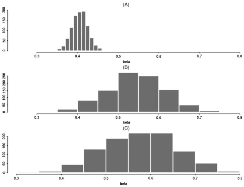
(A) Simulated distribution of mle β̂ from the full retrospective likelihood for pedigrees with four full sibs; simulations centered about the true, β = 0.405. (B) Simulated distribution of mle β̂ from the composite likelihood for four full sibs and (C) pairs of cousins. Results show upward bias of naïve composite likelihood over true β = 0.405.

Fig. 2.

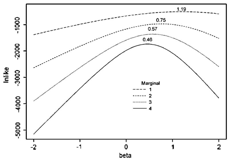
Full retrospective likelihood for simulated data for 4 affecteds sibs, and then “stepped-down” on the same data to naïve marginals for 3, 2, and 1 affected sibs. The mle β̂, printed above each marginal likelihood, is shown to be upward biased over the true simulating value of β = 0.405, with bias increasing as fewer affected subjects are used for an incorrect marginal likelihood.

The cause of this bias is that these “marginal” likelihoods are not correct. They condition only on a subset of affected members per pedigree, not the complete set of affected subjects required to achieve robust adjustment for ascertainment. To see this, consider a pedigree with three affecteds. The correct marginal likelihood for subjects 1 and 2 requires summation of the full likelihood over subject 3,

$$P(g_1,g_2\mid y_1=1,y_2=1,y_3=1)=\sum _{g_3}P(g_1,g_2,g_3\mid y_1=1,y_2=1,y_3=1).$$

This is not the same as what we (and others) have used for the composite likelihood, P(g₁, g₂|y₁ = 1, y₂ = 1). Hence, the simplistic approach we took does not correctly adjust for ascertainment, leading to the observed bias. To construct a correct composite likelihood from correct marginal likelihoods, one would need to sum over the appropriate subjects after evaluating the full retrospective likelihood, negating any computational benefits of the composite approach. The main conceptual, and computational, challenge is the conditioning on the phenotypes of all pedigree members.

For the calculations of both the full retrospective likelihood and the composite likelihood, we assumed that the SNP allele frequencies were known. This is reasonable when prior studies are based on large numbers of control subjects. We did, however, attempt to jointly estimate β and the MAF, p. Because the mle’s of these parameters can be highly negatively correlated, joint estimation can be problematic unless sample sizes are quite large. For this reason, we advocate using controls from a representative population to determine allele frequencies, which are then fixed in the retrospective likelihood when estimating β.

RELATIVE EFFICIENCY OF AFFECTEDS ONLY

We have avoided modeling the contributions from unaffected subjects for RR estimation for several reasons. First, modeling the contributions from unaffected subjects requires more assumptions about the baseline risk of disease (e.g., the intercept in logistic regression), and because highly ascertained pedigrees for linkage studies tend to have many more affected than unaffected subjects, this might require using models that assume a known population prevalence of disease. Yet, we have used the genotypes of the unaffected subjects to constrain the possible genotype configurations of the affected subjects in a pedigree. Nonetheless, this raises questions about the impact on statistical efficiency when ignoring the phenotypes of unaffected subjects. To evaluate this, we derived the relative efficiency of the RR parameter for when unaffecteds are excluded vs. included in the model.

Starting with the retrospective likelihood in expression (2), Fisher’s information for the log RR, β, can be shown to be

$$\text{Info}=E\left[{\left(\frac{R{(G)}^{\prime }}{R(G)}\right)}^2\right]-E{\left[\left(\frac{R{(G)}^{\prime }}{R(G)}\right)\right]}^2,$$

where R(G) is the pedigree RR function, the first derivative is R(G)′ = ∂R(G)/∂β, and E denotes expectation. To take expectations, we used the likelihood to compute the probabilities of the different genotype configurations,

$$P(G\mid Y)=\frac{R(G)P(G)}{{\sum }_{G^{\ast }}R(G^{\ast })P(G^{\ast })}.$$

Fisher’s information can be interpreted as the variance of the score R(G)′/R(G). For relative efficiency calculations, we assumed phenotypes of pedigree members are independent, conditional on the measured genotype,

$$R(G)=\frac{{\prod }_{i=\mathrm{1..}n}P(y_i\mid g_i,)}{{\prod }_{i=\mathrm{1..}n}P(y_i\mid g_i=0)}.$$

To model P(y_i|g_i, ), we used logistic regression with an assumed population prevalence, so that the intercept β₀ is determined once we specify β and the distribution of genotypes (i.e., determined by population allele frequencies for founders of pedigrees).

For a retrospective likelihood based only on affecteds, R(G) = exp{βx}, where x is the sum of the minor alleles among affecteds that have genotype configuration G. It is easy to show that R(G)′/R(G) = x.

For a retrospective likelihood based on both affecteds and unaffecteds,

$$R(G)=\prod _i\frac{{({\text{e}}^{\beta x_i})}^{y_i}}{(1+{\text{e}}^{{\beta }_0+\beta x_i})}(1+{\text{e}}^{{\beta }_0}),$$

where the product is over all genotypes in configuration G, and x_i is the count of minor alleles for subject i. Similar to derivations for logistic regression, it can be shown that R(G)′/R(G) = Σx_i[y_i − P(y_i = 1|x_i)], where P(y = 1|x_i) = e^β₀+βx_i/(1 + e^β₀+βx_i).

Based on the above formulations, we computed the relative efficiency of using phenotypes of only affecteds vs. using phenotypes of both affecteds and unaffecteds, for the two types of pedigrees given in Figure 3. The results in Figure 4 show that the relative efficiency was greater than one (implying affecteds-only analysis is more efficient than analyzing both affecteds and unaffecteds) for both types of pedigrees, for minor allele frequencies ranging 0.05–0.5, for prevalence from 0.01–0.2, and for odds ratios (ORs) of 1.5 and 2.5. This somewhat counterintuitive finding might result from the fact that unaffecteds contribute little information for RR when penetrance is low (e.g., small ORs), and the scores from affected and unaffected pedigree members are negatively correlated.

Fig. 3.

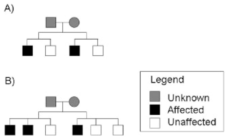
Cousin pedigrees used for calculation of relative efficiencies for affecteds-only vs. affecteds and unaffecteds in retrospective likelihoods.

Fig. 4.

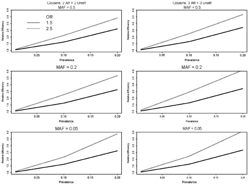
Relative efficiency of retrospective likelihood for affecteds-only vs. affecteds and unaffecteds. Relative efficiency on y-axis is larger than 1.0 when affecteds-only is more efficient than affecteds + unaffecteds for relative risk estimation. MAF = minor allele frequency; OR = odds ratio per allele; Prevalence = population disease prevalence.

APPLICATIONS TO PROSTATE CANCER PEDIGREES

The Mayo Clinic study of the genetic basis of prostate cancer is based on 169 pedigrees collected for linkage analyses, with 2–6 men with prostate cancer per pedigree, giving a total of 469 affected genotyped men in the pedigrees. Also available is a series of 661 hospital-based cases (a group with sporadic prostate cancer and a group with aggressive disease defined by Gleason grade score >7), and 518 population-based controls (for a detailed description of these samples, see [Cunningham et al., 2007]). The controls were used to estimate SNP allele frequencies, and the pedigrees were used in the retrospective likelihood method to estimate per-allele RRs for 28 SNPs previously reported to be associated with prostate cancer, generally in case-control studies. For comparison, the per-allele ORs from the case-control samples were calculated to contrast with results from the retrospective likelihood.

The results from fitting the pedigree retrospective likelihoods are presented in Table I, and graphically illustrated in Figure 5. The estimated per-allele RRs was largest for SNPs on chromosome 8 (RR = 1.85, with MAF = 0.02 for SNP rs698356), similar to prior published reports for SNPs on chromosome 8 [Thomas et al., 2008; Yeager et al., 2007]. The likelihood ratio P-values, illustrated in Figure 5, show multiple statistically significant associations for SNPs on chromosomes 8, 10, 11, and X. Among these 28 SNPs, only four showed evidence of pedigree heterogeneity in baseline risks, with σ̂² ranging 0.5–1.0. After accounting for this heterogeneity, the SNP RR estimates changed only slightly from the estimates that assumed homogeneity in baseline risks (see black squares in Fig. 5).

TABLE I.

Retrospective likelihood parameters estimates for SNPs reported to be associated with prostate cancer

Chromosome	SNP	MAF	β̂	SE(β̂)
2	rs721048	0.18	0.12	0.060
3	rs2660753	0.11	0.11	0.073
6	rs9364554	0.27	0.07	0.055
7	rs10486567	0.24	−0.10	0.062
7	rs6465657	0.47	−0.01	0.050
8	rs979200	0.35	−0.06	0.054
8	rs1016343	0.18	0.23	0.057
8	rs13254738	0.30	0.11	0.052
8	rs6983561	0.02	0.61	0.096
8	rs16901979	0.02	0.61	0.096
8	rs6983267	0.49	−0.06	0.050
8	rs7837328	0.43	0.01	0.051
8	rs7000448	0.36	0.10	0.051
8	rs1447295	0.10	0.36	0.062
8	rs4242382	0.10	0.35	0.063
8	rs10090154	0.10	0.37	0.062
8	rs7005795	0.44	−0.01	0.051
9	rs1571801	0.29	−0.10	0.058
10	rs10993994	0.35	0.18	0.051
10	rs4962416	0.28	−0.03	0.057
11	rs10896449	0.51	−0.24	0.051
17	rs11649743	0.22	−0.15	0.067
17	rs4430796	0.52	−0.17	0.051
17	rs3737559	0.09	0.07	0.084
17	rs1799950	0.06	−0.21	0.124
17	rs1859962	0.51	−0.09	0.050
19	rs2735839	0.14	−0.17	0.081
X	rs5945619	0.30	0.23	0.073

Fig. 5.

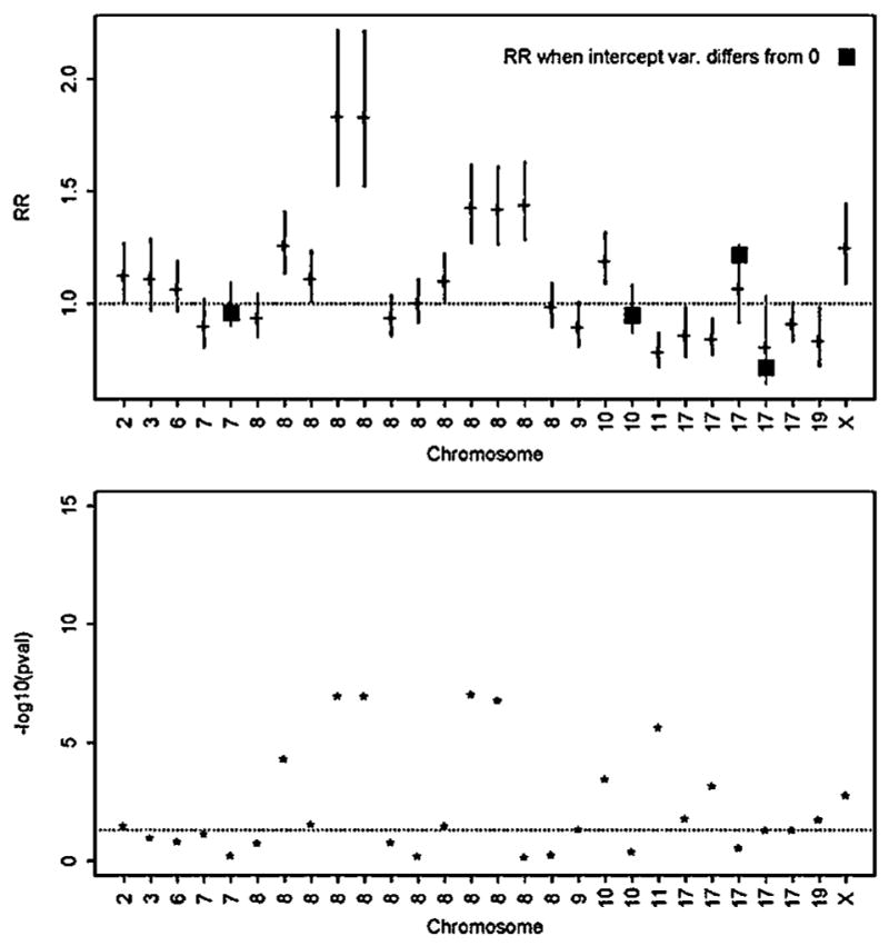
Results from fitting the retrospective likelihood to the Mayo Clinic pedigrees for 28 SNPs reported to be associated with prostate cancer. The upper panel illustrates the mle of the per-allele relative risk (e^β̂) and its 95% confidence interval. For four SNPs, the variance of the baseline risk was estimated to be non-zero; for these four SNPs the mle that accounts for heterogeneity is depicted as a black square. The lower panel is the −log₁₀ (P-value) from the likelihood ratio test of the null hypothesis H_o: β = 0.

To compare the per-allele RRs estimated by the pedigree retrospective likelihood with odds-ratio estimates obtained by case-control studies, we compared our RR estimates with the per-allele OR estimated by two types of cases: aggressive and sporadic, each contrasted with population-based controls. Although there was a slight trend for the ORs from the case-control samples to be slightly larger than those estimated by the retrospective likelihood, illustrated in Figure 6, the 95% confidence intervals for the case-control ORs suggest that much of this is within sampling variation of the parameter estimates. Furthermore, the OR—an approximation to the RR—is greater than the RR when disease is not rare. For example, for a binary exposure variable, if P₊ and P₋ denote the probability of disease among exposed and non-exposed subjects, respectively, then the relative risk is RR = P₊/P₋, in contrast to the odds ratio, OR = RR(1 − P₋)/(1 − P₊). Hence, when RR>1, OR>RR. Overall, our results suggest that the effect-size estimates are generally quite close between the highly ascertained pedigrees and the case-control samples.

Fig. 6.

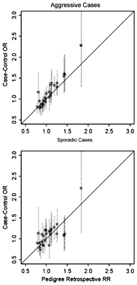
Contrast of results from fitting the retrospective likelihood for 28 SNPs to the Mayo Clinic linkage pedigrees vs. case-control samples. All analyses assumed log-additive effects of a risk-allele, and the broken vertical lines are 95% confidence intervals on the case-control odds ratio estimates.

An advantage of using the NR method to compute the RR parameters for the retrospective likelihood is that the score equations can be used to evaluate the contribution of each pedigree to the estimation procedure. We create a standardized score per pedigree,

$$U_i^{\text{std}}(\widehat{\beta })=U_i(\widehat{\beta })/\sqrt{I_i(\widehat{\beta })}.$$

Because these U scores are evaluated at the mle, they are expected to cluster about zero. Example plots are illustrated in Figure 7. The top panel is for a SNP on chromosome 8 that had the largest RR. This SNP, however, had a small MAF of 0.02. The top panel illustrates that many pedigrees had no risk alleles ( $U_i^{\text{std}}(\widehat{\beta })<0$, with an allele count of “0” in the panel). The standardized U scores above zero tend to be scattered across the number of risk alleles per pedigree, suggesting no dramatic outliers. The lower panel, for a more common risk allele (MAF = 0.30, with RR 1.25), also illustrates that pedigrees with a “0” count of risk alleles have negative U scores, but other pedigrees with risk-allele counts of 1–4 also have U-scores hovering around 0. Overall, there does not appear to be dramatic outlier pedigrees for this SNP.

Fig. 7.

Standardized U scores per pedigree, vs. pedigree number, for two SNPs. The numbers in these figures give the count of the number of risk alleles in each pedigree, and the numbers are colored to make the numbers clearly distinguishable.

DISCUSSION

The benefits of using a retrospective likelihood for highly ascertained pedigrees, such as those collected for pedigree linkage analyses, are well known [Hodge and Elston, 1994; Kraft and Thomas, 2000; Whittemore, 1996], yet often ignored when evaluating the role of common SNPs for high-risk pedigrees. It is important to recognize that using ascertained pedigrees for association analyses per se does not cause a validity problem, yet adjusting for ascertainment is necessary, in contrast to a common practice of simply using one or more affected pedigree members in traditional case-control studies. It is also important to recognize that our proposed methods to estimate RRs are based on comparing the genotype configuration among affected pedigree members to that expected when alleles are randomly segregating in pedigrees, and founder genotypes are expected to fit Hardy-Weinberg proportions. If pedigrees come from different populations with differing allele frequencies, or even if the founders of a single pedigree originate from different populations with differing allele frequencies, one could in theory allow for this heterogeneity by using pedigree-specific or founder-specific allele frequencies. In practice, however, this level of detailed information is rarely known. Furthermore, departure from Mendelian segregation, such as by transmission ratio distortion caused by meiotic drive (i.e., non-random allele segregation at gamete formation) or selective survival, could distort Mendelian segregation, and hence bias RRs. Hence, caution is warranted when interpreting retrospective likelihood RRs; it certainly makes sense to evaluate whether pedigrees originate from different ethnic backgrounds, or whether the measured SNPs are in genes, or have gametic association with genes, that are known to influence survival.

We present novel ways to compute the genotype RR parameters, using a combination of gene-dropping and the Newton-Raphson iterative method. Gene-dropping, a Monte-Carlo method to evaluate a multivariate summation, can be advantageous for large pedigrees for which exact computations would take too much time. One needs to be careful, however, that the sample space of genotype configurations is well covered. For example, when a variant is rare, there is a very small prior probability that multiple pedigree members will be homozygous for the rare variant. Yet, under the alternative that the RR is large, this might not be a rare event. If the number of gene drops is too small, some prior probabilities can be estimated as zero, which means that their corresponding configurations would be treated as impossible, even under the alternative of large risk. Hence, a simple diagnostic of too few gene drops is finding a prior probability estimated as zero. Fortunately, when using the log-additive model for RRs, the sufficient statistic is x, the total count of minor alleles in a pedigree, and many genotype configurations are summed to compute the prior probability of x. So, using this x is also a “smoothing” over the genotype configuration prior probabilities. Perhaps one way to evaluate whether a sufficient number of gene drops was performed is to be sure that a minimum number (e.g., 5) of simulated counts are observed for each level of x.

An alternative approach to improve gene-dropping is importance sampling. Importance sampling is a technique that samples from a distribution other than the target distribution, in order to bias the sampling of “important” configurations, and then corrects this biased sampling by importance weights [Liu, 2001]. For our situation, importance sampling could use a larger MAF than observed, and even a specified magnitude of RR, in order to bias the sampling of the rare configurations, recognizing that the importance weights would be used to weight the genotype configurations to obtain unbiased prior probabilities of the genotype configurations. Importance sampling provides prior probability estimates with smaller variance than the usual gene-dropping estimates. This approach is worthy of further investigation.

Along these lines, a novel type of importance sampling that adjusts for ascertainment was proposed by Clayton [2003]. Instead of conditioning on the phenotypes of all pedigree members, one could improve the statistical efficiency of the estimated parameters by conditioning on the ascertainment process. Because this would require integration over all possible pedigree configurations given the ascertainment process, Clayton suggested randomly sampling pseudo pedigrees. The actual pedigree and its matched set of pseudo pedigrees are then used to create a conditional likelihood score equation, much like the score equation we illustrate for the retrospective likelihood. Because Clayton’s method conditions on less information—the ascertainment process—than the retrospective likelihood, it has the potential to provide parameter estimates with smaller variance. Further evaluation of the strengths and weaknesses of conditioning on an ill-defined ascertainment process, vs. conditioning on phenotypes of all pedigree members, is warranted, particularly, to examine trade-offs of bias and efficiency.

Advantages of computing the score equations for the NR iterations are that variance estimates of the parameters are available and pedigree-specific scores, a by-product of the computations, are useful to evaluate the contribution of each pedigree to the resulting parameter estimates. For our computations with affecteds-only, we found that jointly estimating the MAF and the RR parameter lead to collinearity between these parameters, suggesting that more stable RR estimates can be obtained when SNP allele frequencies can be obtained from representative populations. For large-scale GWA studies, particularly among Caucasians, reliable allele frequencies are often available. Nonetheless, sensitivity analyses can be worthwhile, recognizing that grossly misspecified SNP allele frequencies can bias RR estimates. This concern might be greatest when analyzing pedigrees that have ethnic ancestry that is poorly studied, or when analyzing admixed pedigrees. Further research to evaluate the impact of admixture in pedigrees and poorly specified SNP allele frequencies is warranted.

We evaluated the impact of assuming that affected pedigree members are independent, conditional on their measured SNP genotype, by fitting a model that assumes a random pedigree-specific baseline risk parameter. This random baseline captures heterogeneity in disease risk that might be caused by shared environmental or other genetic risk factors. Among the 28 measured SNPs, only four were found to have non-zero variance estimates for the random baseline; accounting for these random baselines did not substantially change the estimated RRs. Given that multiple SNPs have been identified that increase the risk for prostate cancer, it might be surprising that we did not detect larger effects of heterogeneity when analyzing only one SNP at a time. Kraft and Thomas [2000] showed that the RR estimates from the retrospective likelihood can be biased toward the null when there is heterogeneity in the baseline risks. However, their findings suggested that the bias is small (1–2%) when the baseline heterogeneity is not very large, which might occur for our prostate cancer pedigrees because the RRs associated with each SNP are generally small, on the order of 1.1–1.5. Furthermore, they focused primarily on case-control sib pairs. It is not clear how much of their conclusions can be extrapolated to analyses based on larger pedigrees with only affected subjects. Without unaffected subjects, there is little information on baseline risk, and so bias from heterogeneity in baseline risk might be more difficult to detect.

We also evaluated a marginal approach, based on pairs of affected relatives. However, when conditioning only on the disease status of a pair of relatives, and not the disease status of all pedigree members, the resulting pseudo-composite likelihood leads to biased genotype RRs [although it remains a valid approach to test the null hypothesis of random segregation of alleles, see Meijers-Heijboer et al., 2002]. As illustrated in Figure 2, analyzing a single case from a high-risk family, and ignoring the disease status of the other family members, leads to the greatest bias. Although selecting cases because of a strong family history of disease can provide greater power to detect genetic associations than a random sample of cases [Risch, 2000; Schaid and Rowland, 1998; Teng and Risch, 1999], this “size-biased” sampling also leads to over-estimates of the genetic risk if the ascertainment process is not considered. Unfortunately, this type of sampling is frequently used in reported case-control studies, without adjustment for ascertainment. When sampling multiple affected subjects per pedigree, the retrospective likelihood provides a way to adjust for ascertainment.

Our applications of the retrospective likelihood to the Mayo Clinic pedigrees ascertained for genetic linkage studies of prostate cancer showed that the SNP RR estimates are similar to what has been reported in the literature for case-control studies, and are similar to our own case-control study. This finding suggests that our high-risk pedigrees are not genetically different, in terms SNPs reported to be associated with prostate cancer, from population-based cases. Although one could formally test whether pedigree-based RRs differ statistically from case-control ORs, such as by a likelihood ratio test, plotting point estimates with their confidence intervals makes the comparisons easy to view (see Fig. 6). Further development of the retrospective likelihood to model interactions among SNPs on the RRs, and accounting for linkage and linkage disequilibrium when modeling multiple SNPs in narrow genomic regions, is under development. It is important to recognize that environmental risk factors cancel in the retrospective likelihood when genes and environmental risk factors are independently distributed in the population, and there is no gene-environmental interaction on the RRs. Further developments to model gene-environment interactions in the retrospective likelihood are warranted for some complex diseases, although environmental risk factors for prostate cancer are weak and have been difficult to replicate.

APPENDIX: RETROSPECTIVE MLE BY LINE-SEARCH WITH MLINK

The theoretical derivation of the validity of the MOD score approach is provided by Hodge and Elston [1994]. They show that the maximized retrospective likelihood is a MOD score, which is the ratio of a likelihood under the alternative hypothesis (in our case, modeling a causal locus as complete linkage disequilibrium between a measured SNP allele and an underlying disease allele), and a likelihood under the null hypothesis of no linkage and no linkage disequilibrium. This means that mlink must be run twice. Step 1 below illustrates the mlink datafile for calculating the log-likelihood for a causal locus, and Step 2 for the calculating the log-likelihood for the null hypothesis. When using affecteds only, affecteds are coded with affection = 2, and all others with affection = 0. In this case, the absolute penetrances are not relevant, only the ratio of penetrances. For this reason, the penetrance for the N/N genotype is arbitrary; we set it to 0.1. The examples below are illustrated for: (1) a SNP risk allele with frequency of 0.2; (2) complete LD of SNP allele 2 with disease-locus allele D; (3) a per-allele RR of 2. The mlink output from Step 1 gives lnlike_causal, and from Step 2, lnlike_null. The retrospective log-likelihood is computed as lnlike_{retrospective} = lnlike_causal − lnlike_null. To determine the maximum likelihood estimator of the genotype RR, these two steps must be computed for a range of RRs to determine which value maximizes lnlike_{retrospective}.

Step 1: mlink datafile for a causal locus: complete LD of SNP allele 2 with underlying disease locus allele D, and complete linkage (recombination fraction = 0.0)

2 0 0 5 # No. of loci, risk locus, sexlinked (if 1), program

0 0.0 0.0 1 # Haplotypes for LD

1 2 # Locus order

1 2 # Disease locus with alleles N = normal, D = Disease

1 # No. of liability classes

0.1 0.2 0.4 # relative penetrances for N/N (arbitrary), N/D (rr = 2), D/D (rr = 4)

3 2 # SNP with alleles 1 (low risk) and 2 (high risk)

0.8 0.0 0.0 0.2 # haplotype freqs for N-1, N-2, D-1, D-2

0 0 # Sex difference, interference (if 1 or 2)

0.0 # Recombination values, complete linkage

1 .5 0.0 # Rec varied, increment, finishing value

Step 2: mlink datafile under null of no LD and no linkage (recombination fraction = 0.5)

2 0 0 5 # No. of loci, risk locus, sexlinked (if 1), program

0 0.0 0.0 0 # No LD

1 2 # Locus order

1 2 # # Disease locus with alleles N = normal, D = Disease

0.8 0.2 # Disease locus allele frequencies

1 # No. of liability classes

0.1 0.2 0.4 # relative penetrances for N/N (arbitrary), N/D (rr = 2), D/D (rr = 4)

3 2 # SNP with alleles 1 (low risk) and 2 (high risk)

0.8 0.2 # SNP allele frequencies

0 0 # Sex difference, interference (if 1 or 2)

0.5 # Recombination values, no linkage

1 0.60000 0.5000 # Rec varied, Increment, Finishing value

References

- Botstein D, White RL, Skolnick M, Davis RW. Construction of a genetic linkage map in man using restriction fragment length polymorphisms. Am J Hum Genet. 1980;32:314–331. [PMC free article] [PubMed] [Google Scholar]
- Carayol J, Bonaiti-Pellie C. Estimating penetrance from family data using a retrospective likelihood when ascertainment depends on genotype and age of onset. Genet Epidemiol. 2004;27:109–117. doi: 10.1002/gepi.20007. [DOI] [PubMed] [Google Scholar]
- Chanock SJ, Manolio T, Boehnke M, Boerwinkle E, Hunter DJ, Thomas G, Hirschhorn JN, Abecasis G, Altshuler D, Bailey-Wilson JE, et al. Replicating genotype-phenotype associations. Nature. 2007;447:655–660. doi: 10.1038/447655a. [DOI] [PubMed] [Google Scholar]
- Chatterjee N, Wacholder S. A marginal likelihood approach for estimating penetrance from kin-cohort designs. Biometrics. 2001;57:245–252. doi: 10.1111/j.0006-341x.2001.00245.x. [DOI] [PubMed] [Google Scholar]
- Chatterjee N, Shih J, Hartge P, Brody L, Tucker M, Wacholder S. Association and aggregation analysis using kin-cohort designs with applications to genotype and family history data from the Washington Ashkenazi Study. Genet Epidemiol. 2001;21:123–138. doi: 10.1002/gepi.1022. [DOI] [PubMed] [Google Scholar]
- Chatterjee N, Hartge P, Wacholder S. Adjustment for competing risk in kin-cohort estimation. Genet Epidemiol. 2003;25:303–313. doi: 10.1002/gepi.10269. [DOI] [PubMed] [Google Scholar]
- Clayton D. Conditional likelihood inference under complex ascertainment using data augmentation. Biometrika. 2003;90:976–981. [Google Scholar]
- Clerget-Darpoux F, Elston RC. Are linkage analysis and the collection of family data dead? Prospects for family studies in the age of genome-wide association. Hum Hered. 2007;64:91–96. doi: 10.1159/000101960. [DOI] [PubMed] [Google Scholar]
- Cunningham JM, Hebbring SJ, McDonnell SK, Cicek MS, Christensen GB, Wang L, Jacobsen SJ, Cerhan JR, Blute ML, Schaid DJ, et al. Evaluation of genetic variations in the androgen and estrogen metabolic pathways as risk factors for sporadic and familial prostate cancer. Cancer Epidemiol Biomarkers Prev. 2007;16:969–978. doi: 10.1158/1055-9965.EPI-06-0767. [DOI] [PubMed] [Google Scholar]
- Gail MH. Estimation and interpretation of models of absolute risk from epidemiologic data, including family-based studies. Lifetime Data Anal. 2008;14:18–36. doi: 10.1007/s10985-007-9070-0. [DOI] [PubMed] [Google Scholar]
- Gail MH, Pee D, Benichou J, Carroll R. Designing studies to estimate the penetrance of an identified autosomal dominant mutation: cohort, case-control, and genotyped-proband designs. Genet Epidemiol. 1999a;16:15–39. doi: 10.1002/(SICI)1098-2272(1999)16:1<15::AID-GEPI3>3.0.CO;2-8. [DOI] [PubMed] [Google Scholar]
- Gail MH, Pee D, Carroll R. Kin-cohort designs for gene characterization. J Natl Cancer Inst Monogr. 1999b;26:55–60. doi: 10.1093/oxfordjournals.jncimonographs.a024227. [DOI] [PubMed] [Google Scholar]
- Geppert S, Koller S. In: Erbmathematik; Theorie der Vererbung in Bevölkerung und Sippe. Meyer Qu., editor. Leipzig; 1938. [Google Scholar]
- Hodge SE, Elston RC. Lods, wrods, and mods: the interpretation of lod scores calculated under different models. Genet Epidemiol. 1994;11:329–342. doi: 10.1002/gepi.1370110403. [DOI] [PubMed] [Google Scholar]
- Kraft P, Thomas D. Bias and efficiency in family-based gene-characterization studies: conditional, prospective, retrospective, and joint likelihoods. Am J Hum Genet. 2000;66:1119–1131. doi: 10.1086/302808. [DOI] [PMC free article] [PubMed] [Google Scholar]
- Lange K. Mathematical and Statistical Methods for Genetic Analysis. New York: Springer; 2002. [Google Scholar]
- Li C, Sacks L. The derivation of joint distribution and correlation between relatives by the use of stochastic matrices. Biometrics. 1954;10:347–360. [Google Scholar]
- Lindsay BG. Composite likelihood methods. Contemp Math. 1988;80:221–239. [Google Scholar]
- Liu J. Monte Carlo Strategies in Scientific Computing. New York: Springer-Verlag; 2001. [Google Scholar]
- Matise TC, Chen F, Chen W, De La Vega FM, Hansen M, He C, Hyland FC, Kennedy GC, Kong X, Murray SS, et al. A second-generation combined linkage physical map of the human genome. Genome Res. 2007;17:1783–1786. doi: 10.1101/gr.7156307. [DOI] [PMC free article] [PubMed] [Google Scholar]
- Meijers-Heijboer H, van den Ouweland A, Klijn J, Wasielewski M, de Snoo A, Oldenburg R, Hollestelle A, Houben M, Crepin E, van Veghel-Plandsoen M, et al. Low-penetrance susceptibility to breast cancer due to CHEK2(*)1100delC in noncarriers of BRCA1 or BRCA2 mutations. Nat Genet. 2002;31:55–59. doi: 10.1038/ng879. Epub Apr 22, 2002. [DOI] [PubMed] [Google Scholar]
- Millikan RC, Hummer AJ, Wolff MS, Hishida A, Begg CB. HER2 codon 655 polymorphism and breast cancer: results from kin-cohort and case-control analyses. Breast Cancer Res Treat. 2005;89:309–312. doi: 10.1007/s10549-004-2171-5. [DOI] [PubMed] [Google Scholar]
- Moore DF, Chatterjee N, Pee D, Gail MH. Pseudo-likelihood estimates of the cumulative risk of an autosomal dominant disease from a kin-cohort study. Genet Epidemiol. 2001;20:210–227. doi: 10.1002/1098-2272(200102)20:2<210::AID-GEPI4>3.0.CO;2-I. [DOI] [PubMed] [Google Scholar]
- Pearson TA, Manolio TA. How to interpret a genome-wide association study. J Am Med Assoc. 2008;299:1335–1344. doi: 10.1001/jama.299.11.1335. [DOI] [PubMed] [Google Scholar]
- Rabinowitz D. A pseudolikelihood approach to correcting for ascertainment bias in family studies. Am J Hum Genet. 1996;59:726–730. [PMC free article] [PubMed] [Google Scholar]
- Risch HA, McLaughlin JR, Cole DE, Rosen B, Bradley L, Fan I, Tang J, Li S, Zhang S, Shaw PA, et al. Population BRCA1 and BRCA2 mutation frequencies and cancer penetrances: a kin-cohort study in Ontario, Canada. J Natl Cancer Inst. 2006;98:1694–1706. doi: 10.1093/jnci/djj465. [DOI] [PubMed] [Google Scholar]
- Risch N. Searching for genetic determinants in the new millennium. Nature. 2000;405:847–856. doi: 10.1038/35015718. [DOI] [PubMed] [Google Scholar]
- Risch N, Merikangas K. The future of genetic studies of complex human diseases. Science. 1996;273:1516–1517. doi: 10.1126/science.273.5281.1516. [DOI] [PubMed] [Google Scholar]
- Saunders CL, Begg CB. Kin-cohort evaluation of relative risks of genetic variants. Genet Epidemiol. 2003;24:220–229. doi: 10.1002/gepi.10235. [DOI] [PubMed] [Google Scholar]
- Schaid DJ, Rowland CM. Use of parents, sibs, and unrelated controls for detection of associations between genetic markers and disease. Am J Hum Genet. 1998;63:1492–1506. doi: 10.1086/302094. [DOI] [PMC free article] [PubMed] [Google Scholar]
- Sigurdson AJ, Hauptmann M, Chatterjee N, Alexander BH, Doody MM, Rutter JL, Struewing JP. Kin-cohort estimates for familial breast cancer risk in relation to variants in DNA base excision repair, BRCA1 interacting and growth factor genes. BMC Cancer. 2004;4:9. doi: 10.1186/1471-2407-4-9. [DOI] [PMC free article] [PubMed] [Google Scholar]
- Teng J, Risch N. The relative power of family-based and case-control designs for linkage disequilibrium studies of complex diseases. II. Individual genotyping. Genome Res. 1999;9:234–241. [PubMed] [Google Scholar]
- Thomas G, Jacobs KB, Yeager M, Kraft P, Wacholder S, Orr N, Yu K, Chatterjee N, Welch R, Hutchinson A, et al. Multiple loci identified in a genome-wide association study of prostate cancer. Nat Genet. 2008;40:310–315. doi: 10.1038/ng.91. [DOI] [PubMed] [Google Scholar]
- Thompson E. Pedigree Analysis in Human Genetics. Baltimore: The Johns Hopkins University Press; 1986. [Google Scholar]
- Varin C. On composite marginal likelihoods. AStA Adv in Stat Anal. 2008;92:1–28. [Google Scholar]
- Wacholder S, Hartge P, Struewing JP, Pee D, McAdams M, Brody L, Tucker M. The kin-cohort study for estimating penetrance. Am Journal of Epidemiol. 1998;148:623–630. doi: 10.1093/aje/148.7.623. [DOI] [PubMed] [Google Scholar]
- Wang Y, Clark LN, Louis ED, Mejia-Santana H, Harris J, Cote LJ, Waters C, Andrews H, Ford B, Frucht S, et al. Risk of Parkinson disease in carriers of parkin mutations: estimation using the kin-cohort method. Arch Neurol. 2008;65:467–474. doi: 10.1001/archneur.65.4.467. [DOI] [PMC free article] [PubMed] [Google Scholar]
- Webb EL, Rudd MF, Houlston RS. Case-control, kin-cohort and meta-analyses provide no support for STK15 F31I as a low penetrance colorectal cancer allele. Br J Cancer. 2006a;95:1047–1049. doi: 10.1038/sj.bjc.6603382. [DOI] [PMC free article] [PubMed] [Google Scholar]
- Webb EL, Rudd MF, Houlston RS. Case-control, kin-cohort and meta-analyses provide no support for STK15 F31I as a low penetrance colorectal cancer allele. Br J Cancer. 2006b;95:1047–1049. doi: 10.1038/sj.bjc.6603382. [DOI] [PMC free article] [PubMed] [Google Scholar]
- Webb EL, Rudd MF, Sellick GS, El Galta R, Bethke L, Wood W, Fletcher O, Penegar S, Withey L, Qureshi M, et al. Search for low penetrance alleles for colorectal cancer through a scan of 1467 non-synonymous SNPs in 2575 cases and 2707 controls with validation by kin-cohort analysis of 14 704 first-degree relatives. Hum Mol Genet. 2006c;15:3263–3271. doi: 10.1093/hmg/ddl401. [DOI] [PubMed] [Google Scholar]
- Whittemore AS. Genome scanning for linkage: an overview. Am J Hum Genet. 1996;59:704–716. [PMC free article] [PubMed] [Google Scholar]
- Yeager M, Orr N, Hayes RB, Jacobs KB, Kraft P, Wacholder S, Minichiello MJ, Fearnhead P, Yu K, Chatterjee N, Wang Z, Welch R, Staats BJ, Calle EE, Feigelson HS, Thun MJ, Rodriguez C, Albanes D, Virtamo J, Weinstein S, Schumacher FR, Giovannucci E, Willett WC, Cancel-Tassin G, Cussenot O, Valeri A, Andriole GL, Gelmann EP, Tucker M, Gerhard DS, Fraumeni JF, Hoover R, Hunter DJ, Chanock SJ, Thomas G. Genome-wide association study of prostate cancer identifies a second risk locus at 8q24. Nat Genet. 2007;39:645–649. doi: 10.1038/ng2022. [DOI] [PubMed] [Google Scholar]