

Abstract
The state-of-the-art technology for theoretically exact local computed tomography (CT) is to reconstruct an object function using the truncated Hilbert transform (THT) via the projection onto convex sets (POCS) method, which is iterative and computationally expensive. Here we propose to reconstruct the object function using the THT via singular value decomposition (SVD). First, we review the major steps of our algorithm. Then, we implement the proposed SVD method and perform numerical simulations. Our numerical results indicate that our approach runs two orders of magnitude faster than the iterative approach and produces an excellent region-of-interest (ROI) reconstruction that was previously impossible, demonstrating the feasibility of localized pre-clinical and clinical CT as a new direction for research on exact local image reconstruction. Finally, relevant issues are discussed.
Keywords: Computed tomography (CT), truncated Hilbert transform (THT), singular value decomposition (SVD), regularization, local image reconstruction
I. Introduction
Let μ(r⃗) be a smooth function on a compact support Ω ⊂ R2, with r⃗ = (r1, r2) and R2 denoting the two-dimensional (2D) real space. Define the line integral
| (1) |
for s ∈ R and 0 ≤ ϕ < π, where u⃗(ϕ) = (cos ϕ, sin ϕ) and u⃗⊥ = (ϕ) (−sin ϕ, cos ϕ) . p(s, ϕ) can be extended to ϕ ∈ R with p(s, ϕ + π) = p(−s, ϕ). For a fixed ϕ0, by Noo et al. [1], the backprojection of differential data
| (2) |
can be expressed as the Hilbert transform of μ along the line L through r⃗0 which is parallel to n⃗ (−sin ϕ0, cos ϕ0):
| (3) |
where “PV” indicates the Cauchy principal value, and HL the Hilbert Transform along the line L.
For clinical applications, it is highly desirable to minimize the x-ray dose during a CT scan because the ionizing radiation may induce cancers and genetic damage in the patient. Naturally, the limited data reconstruction strategy can be used to reduce the x-ray dose significantly. This strategy may improve the data acquisition speed at the same time. Let us denote the 2D μ(r⃗) on a line L as f(x) and b(r⃗0) as g(x) where x is the one-dimensional (1D) coordinate along the line L. Assume the intersection of the compact support and the line L is the interval (c1, c2) with c1 < c2, which imply that f(x) = 0 for x ∉ (c1, c2). Also, let us assume that the backprojection of differential data can be exactly obtained from the original projection data through the interval (c3, c4) with c3 < c4. All the intervals (c3, c4) form a sub-region inside the compact support of μ(r⃗). This sub-region usually is called the region-of-interest (ROI) or field of view (FOV). Recovering the object function inside the ROI is generally called local image reconstruction. Using the above notations, Eq. (3) can be rewritten as
| (4) |
In this paper, we call g(x) on the interval (c3, c4) as the truncated Hilbert Transform (THT). By the sufficient reconstruction condition of the backprojection filtration algorithms [1-3], f(x) can be exactly reconstructed on the whole compact support interval (c1, c2) if c3 < c1 < c2 < c4 (Fig. 1(a)). Lately, Defrise et al. [4] proposed the enhanced condition that f(x) can be exactly reconstructed on the interval (c1, c4) if c3 < c1 < c4 < c2 (Fig. 1(b)). In the case of c1 < c3 < c4 < c2, it is the well known local reconstruction problem that does not have a unique solution [5]. However, we recently proved that the exact reconstruction is possible in this case with some prior knowledge, which leads to many clinical or pre-clinical applications [6, 7]. If there exist real numbers c1 < c3 < c5 < c4 < c2 and f(x) is known on the interval (c3, c5), f(x) can be exactly reconstructed on the interval [c5, c4) (Fig. 1(c)). Although the projection onto convex sets (POCS) method has been employed to recover f(x) iteratively [4, 7], it is computationally very expensive. To our best knowledge, there is no analytic method to recover f(x) in the cases of c3 < c1 < c4 < c2 and c1 < c3 < c5 < c4 < c2. Therefore, it is crucial to develop a fast yet stable method for the local reconstruction using the THT.
Figure 1.
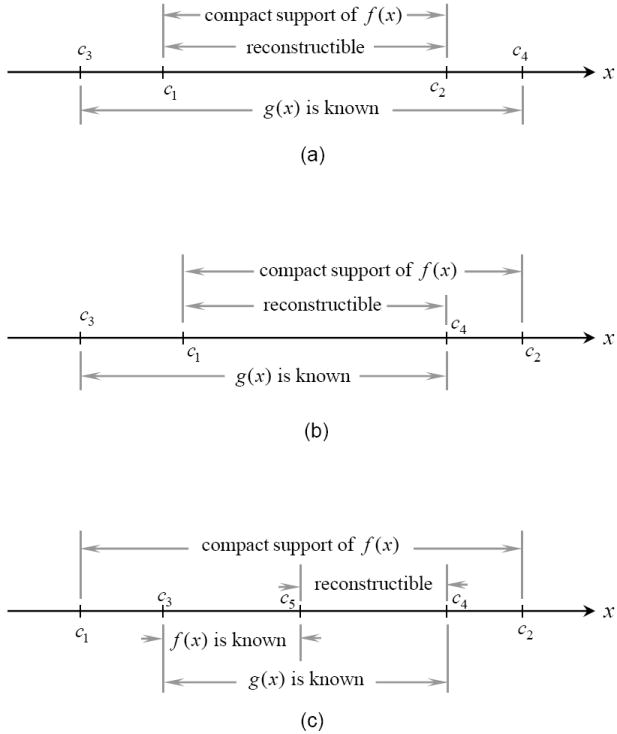
Various exact reconstruction regions using the truncated Hilbert Transform based on different sufficient conditions. (a) The exact reconstruction region by Noo et al.[1], (b) that by Defrise et al. [4], and (c) that by our group [7].
In this paper, we propose to recover f(x) using the THT via singular value decomposition (SVD) [8, 9]. In the next section, we review the major steps of our algorithm. In the third section, we demonstrate in the numerical simulation that the SVD method is superior to the POCS method in terms of computational efficiency. In the last section, we discuss relevant issues and conclude the paper.
II. Singular Value Decomposition
For our local reconstruction problem, the THT g(x) in Eq. (4) can be exactly computed from a truncated projection dataset via Eq. (2). That is, b(r⃗0) is computed only from the projection data whose paths go through the point r⃗0. For brevity, we assume that the readers are familiar with the backprojection process [1, 2, 10] and focus on how to recover f(x) from Eq.(4).
To introduce the SVD method for reconstruction of f(x) , we first discretize the real x -axis with a uniform sampling interval xδ. Both f(x) and g(x) are then sampled on the discrete points on the x -axis. Denote f(x) on the sampling points in (c1, c2) as f1, f2, ⋯ fn ⋯, fN and g(x) on the sampling points in (c3, c4) as g1, g2, ⋯ gm, ⋯ gM. Eq.(4) can be written as
| (5) |
where
| (6) |
| (7) |
| (8) |
In Eqs.(6) and (7), “T” represents the transpose operator. In Eq.(8), hm,n is the weighting coefficient. Let x f,n and xg,m be the corresponding coordinates on the x -axis for fn and gm. Based on the discrete Hilbert Kernel developed in [11], it is easy to show that
| (9) |
With
| (10) |
The case lm,n = 0 in Eq.(9) exactly corresponds to the singular point in the Cauchy principal integral in Eq.(4). If some fn are known, we may divide F into two parts
| (11) |
where Fu is the unknown part while Fk is the known part. Correspondingly, the coefficient matrix H can be divided into the two parts
| (12) |
Then, we immediately arrives at a linear equation system
| (13) |
with G̃ = G − Hk Fk, H̃ = Hu and F̃ = Fu. It should be pointed out that Eq. (13) covers all the reconstruction problems illustrated in Figure 1.
In most of our applications, Eq. (13) is not well-posed in general. Hence, we cannot solve F̃ satisfactorily using the common least-square method. Assuming that the dimension of F̃ is Ñ, the dimension of G̃ and H̃ are M and M × Ñ, respectively. According to the SVD theory, the matrix H̃ has a SVD in the following form [8, 9]
| (14) |
where U and V are orthogonal matrices of M × M and Ñ × Ñ respectively, and Λ is a M × Ñ diagonal matrix whose diagonal elements with λq satisfying λ1 ≥ ⋯ ≥ λq ≥ ⋯ λQ with Q = min(M, Ñ) . In this way, we have a stable numerical solution for F̃ [8, 9],
| (15) |
where Λ−1 is an orthogonal matrix of Ñ × M whose diagonal elements is defined as
| (16) |
and ε > 0 is a free constant parameter. The method defined by Eqs. (15) and (16) is called truncated SVD (TSVD) [8], which is a special case of regularization. The more general regularization method is to solve F̃ by minimizing the object function
| (17) |
where S is a matrix of Ñ × Ñ, and ξ a free constant parameter. When S is a unit diagonal matrix, the solution of (17) can be expressed as Eq. (15) except that
| (18) |
Eqs. (15) and (18) is called the Tikhonov regularization [8]. Both ε in Eq. (16) and ξ in Eq. (18) play the same role in controlling the “smoothness” of the regularized solution.
III. Numerical Simulation
The SVD method described above was implemented in MatLab on a regular PC (1.0G memory, 2.8G CPU). As illustrated in Figure 2, the function μ(r⃗) is an axial slice of the FORBILD thorax phantom [12] with two small ellipses added into the heart to make it more challenging for reconstruction, which was also used in the paper by Defrise et al. [4]. Non-truncated fan-beam projection data of 1200 directions were analytically computed over a full-scan range, covering a field of view with a radius of 25cm. The radius of the scanning trajectory was assumed to be 57cm. The distance between the x-ray source and detector was 114 cm. There were 1200 detector elements along an 80cm line detector. Hence, the backprojection function at any point can be calculated along any line to simulate different field of view. In our simulation, a full reconstruction of the phantom was represented as a matrix of 1136×636. Our experimental design consisted of two stages. In the first stages, we reconstructed the ROIs only using the available THT datasets. In the second stages, we introduced a priori information into the SVD method to improve the image quality. Specifically, we imposed the exact support constraint in the SVD reconstruction, which was the same as done in the POCS reconstruction. For better comparison between the SVD and POCS methods, we re-simulated all the cases described in [7] using both the methods. Based on our experience, the TSVD and Tikhonov regularization do not differ significantly. Hence, in the following we only present our results using TSVD with ε = 0.05.
Figure 2.
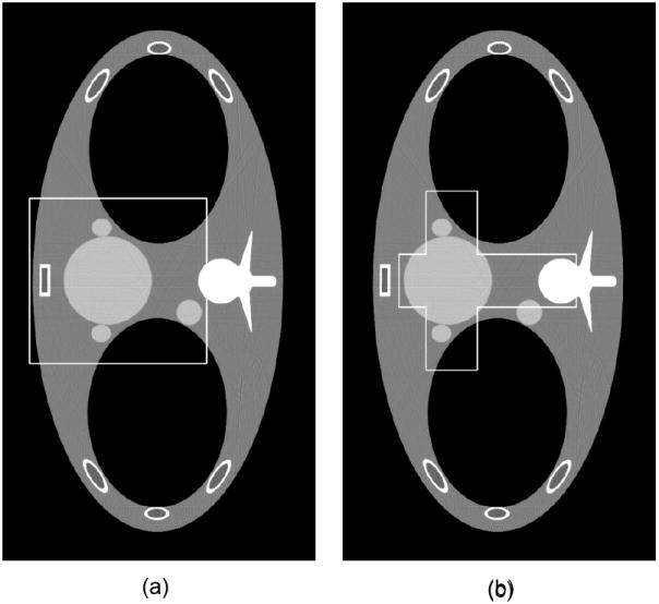
Representative slice of the thorax phantom [6]. (a) A rectangular ROI satisfying Defrise’s condition in [4] and (b) a cross-shaped ROI inside the object compact support with some known region satisfying our condition in [7]. The display window is [0.9,1.1] in both the cases.
Figure 3 shows the images that were reconstructed within a rectangular ROI of 337×362 pixels indicated in Figure 2(a), while Figure 4 are the images reconstructed within a cross-shaped ROI of 366×362 pixels indicated in Figure 2(b). We assumed that in the Figure 2(b) the central rectangular part of the cross-shaped ROI was known. To validate the stability of the SVD method, the above results were repeated by adding Poisson noise with 2 × 10⁵ photons per incident ray [13]. The corresponding images are presented in Figures 3 and 4. It should be pointed out that the known images in the rectangular parts in Figure 2(b) were from the reconstructed images using the conventional FBP method from the same noise-free/noisy datasets. Also, the images in Figure 4 were reconstructed along two groups of parallel lines which are horizontal and vertical respectively. While the TSVD method only took 1.43s and 2.92s to recover Figure 3(a) and Figure 4(a) respectively, the POCS method used 252.11s and 314.39s to reconstruct Figure 3(b) and Figure 4(b). Since the build-in SVD decomposition and Matrix operations (for both SVD and POCS methods) in Matlab are well optimized, based on our experience the SVD method proposed in this paper can reduce the computational time by two orders of magnitude, as compared to that required by the POCS method with comparable simulation parameters [7].
Figure 3.
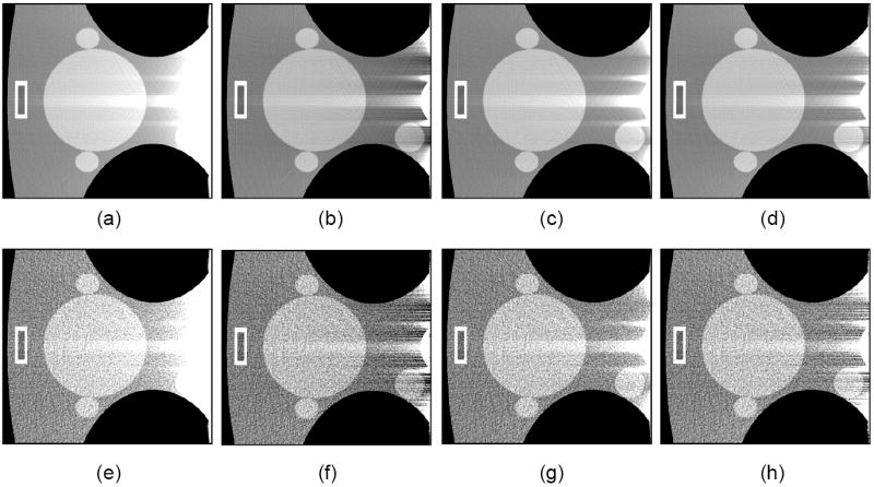
Reconstructed results in the rectangular ROI shown in Figure 2(a). (a) The image reconstructed using the TSVD method without any prior information, (b) the counterpart of (a) reconstructed using the POCS method; (c) an improved version of (a) reconstructed using the TSVD with the known compact support; (d) the counterpart of (c) reconstructed using the POCS method. (e)-(h) are the counterparts of (a)-(d) in the noisy data case. The display window is [0.9,1.1].
Figure 4.
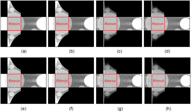
Reconstructed results in the cross-shaped ROI shown in Figure 2(b), which are arranged in the way similar to Figure 3.
In reference to Figures 3 and 4, the following comments are in order. First, all the reconstructed images using either the SVD or POCS methods produced streak artifacts, especially near the regions where the truncated Hilbert transforms were not available, that is, near the point c3 or c4. According to Defrise et al. [4], these artifacts were caused by the high contrast structures located just outside the field of view. This argument can be also made based on the stability analysis in our previous work [7] or that by Defrise et al. [4]. Second, from the reconstructed images with and without noise, we conclude that reconstructed images using the SVD method have an image quality comparable to that with the POCS method in terms of contrast resolution and image noise. This evidence is in strong support of the exact reconstruction claims made by Defrise et al. [4] and our group [7]. Third, although we assumed the support of the object function when the SVD method was applied, it is not necessary to know the exact support. In fact, we can assume a larger support to cover the exact support in practical applications. Fourth, prior information is helpful to improve the image quality. Although the SVD method is not as flexible as the POCS method to incorporate the prior information, we can optimize the transform matrix S in Eq. (17) subject to additional constraints. However, these need more theoretical analysis and numerical tests. We will work along this direction and report our results in the future.
IV. Discussions and Conclusion
In the classic references on SVD [8, 9], it was assumed that the dimension of H̃ satisfying M ≥ Ñ which implies that the number of measured data should not smaller than that of the unknown variables. For the reconstruction problem from THT, this requires that (a) (c4 − c3) > (c2 − c1) in the case of c3 < c1 < c4 < c2 and (b) (c4 − c3) > (c2 − c5) + (c3 − c1) in the case of c1 < c3 < c5 < c4 < c2. Hansen derived the perturbation bounds to demonstrate the stability of SVD for recovering all the Ñ variables with M ≥ Ñ. Under this condition M ≥ Ñ, Hansen proved that if δ is the ∥•∥2 norm of the error of the measured data, the ∥•∥2 norm of the reconstruction error will be bounded by a constant multiple of δ. This reconstruction error bound is better than what was obtained in [4] and [7], which is only less than a constant multiple of a fractional power of δ. On the other hand, the most common case is M < Ñ for the reconstruction problem from the THT that cannot be covered by Hansen’s results. Although the SVD method can not stable recover all the Ñ variables, as illustrated in the this study, it can obtain a stable estimation for a majority of the unknown variables, which have been theoretically established [4, 7]. We will report more theoretical analysis and estimation results on the perturbation bounds in the near future.
In the review process of this manuscript, a reviewer brought to our attention a conference abstract by Kudo [14], in which he reported a uniqueness result on the interior reconstruction. Specifically, he claimed the following theorem that “Let S be a pathwise connected set (non-convex set is allowed) which corresponds to a ROI. Let H be a subset of S on which the 1-D Hilbert transform Hf (x, y) is accessible using the DBP method. Then, the object f (x, y) is uniquely determined on S if the following two conditions are satisfied. (1) f (x, y) is known a priori on the set K = S \ H. (2) There exists a subset (possibly a small subset) of S (denoted by B) on which both Hf (x, y) and f (x, y) are known.” In Nov. 2007, Kudo et al. presented their latest results along this line [15], in which they excluded the lower case in Figure 1 (c) (a non-convex ROI case) that is a counter-example to the theorem in [14]. Additionally, in [14] Kudo did not request that set B be of non-zero measure and did not mention a technique to achieve exact ROI reconstruction. As a matter of fact, after reading the paper by Defrise et al. [4] in May, 2006, we immediately had the hypothesis that the exact interior reconstruction is solvable for any set B, and considered it as a key to solve our long-standing conjecture on the correctness of an exact FBP helical cone-beam formula that utilizes curved filtering paths [16]. However, we have been unable to perform analytic continuation from knowledge on a set of zero measure. Hence, our work on exact interior reconstruction should be considered as original.
In conclusion, local image reconstruction using the THT makes it possible to recover a ROI exactly under the condition that there is some known region in the ROI. In practice, we may find that the known information inside a sub-region of the ROI, such as air around a tooth, water in a device, or metal in a semiconductor. Our method represents the-state-of-art understanding of exact local CT. Because it requires the minimum amount of projection data, this approach helps not only reduce the x-ray radiation exposure but also improve the data acquisition speed. The SVD method we proposed here offers an efficient and stable way for this purpose, which is the main contribution of this technical note. More work will be conducted for further improvement of image quality along this direction.
Acknowledgments
This work is partially supported by NIH/NIBIB grants (EB002667, EB004287 and EB007288).
Contributor Information
Hengyong Yu, Email: hengyong-yu@ieee.org.
Yangbo Ye, Email: yangbo-ye@uiowa.edu.
Ge Wang, Email: ge-wang@ieee.org.
References
- 1.Noo F, Clackdoyle R, Pack JD. A two-step Hilbert transform method for 2D image reconstruction. Physics in Medicine and Biology. 2004;49(17):3903–3923. doi: 10.1088/0031-9155/49/17/006. [DOI] [PubMed] [Google Scholar]
- 2.Ye YB, Zhao SY, Yu HY, Wang G. A General Exact Reconstruction for Cone-Beam CT via Backprojection-Filtration. IEEE Transactions on Medical Imaging. 2005;24(9):1190–1198. doi: 10.1109/TMI.2005.853626. [DOI] [PubMed] [Google Scholar]
- 3.Li L, Tang J, Xing YX, Cheng JP. An exact reconstruction algorithm in variable pitch helical cone-beam CT when PI-line exists. Journal of X-ray Science and Technology. 2006;14:109–118. [Google Scholar]
- 4.Defrise M, Noo F, Clackdoyle R, Kudo H. Truncated Hilbert transform and image reconstruction from limited tomographic data. Inverse Problems. 2006;22(3):1037–1053. [Google Scholar]
- 5.Natterer F. Classics in applied mathematics. Vol. 32. Philadelphia: Society for Industrial and Applied Mathematics; 2001. The Mathematics of Computerized Tomography. cm. [Google Scholar]
- 6.Wang G, Ye YB, Yu HY. General VOI/ROI Reconstruction Methods and Systems using a Truncated Hilbert Transform. Patent disclosure submitted to Virginia Tech Intellectual Properties on May 15, 2007. 2007 [Google Scholar]
- 7.Ye YB, Yu HY, Wei YC, Wang G. A General Local Reconstruction Approach Based on a Truncated Hilbert Transform. International Journal of Biomedical Imaging. 2007;2007:Article ID: 63634–8. doi: 10.1155/2007/63634. [DOI] [PMC free article] [PubMed] [Google Scholar]
- 8.Hansen PC. Truncated Singular Value Decomposition Solutions To Discrete Ill-Posed Problems With Ill-Determined Numerical Rank. Siam Journal On Scientific And Statistical Computing. 1990;11(3):503–518. [Google Scholar]
- 9.Hansen PC. Regularization, Gsvd And Truncated Gsvd. Bit. 1989;29(3):491–504. [Google Scholar]
- 10.Yu HY, Ye YB, Zhao SY, Wang G. A backprojection-filtration algorithm for nonstandard spiral cone-beam CT with an n-PI-window. Physics in Medicine and Biology. 2005;50(9):2099–2111. doi: 10.1088/0031-9155/50/9/012. [DOI] [PubMed] [Google Scholar]
- 11.Yu HY, Wang G. Studies on implementation of the Katsevich algorithm for spiral cone-beam CT. Journal of X-ray Science and Technology. 2004;12(2):96–117. [Google Scholar]
- 12.Sourbelle K. Thorax Phantom. http://www.imp.uni-erlangen.de/forbild/english/results/index.htm.
- 13.Yu HY, Ye YB, Zhao SY, Wang G. Local ROI Reconstruction via Generalized FBP and BPF Algorithms along more Flexible Curves. International Journal of Biomedical Imaging. 2006;2006(2):Article ID: 14989–7. doi: 10.1155/IJBI/2006/14989. [DOI] [PMC free article] [PubMed] [Google Scholar]
- 14.Kudo H. Analytical image reconstruction methods for medical tomography – Recent advances and a new uniqueness result. Mathematical Aspects of Image Processing and Computer Vision. 2006 [Google Scholar]
- 15.Kudo H, Courdurier M, Noo F, Defrise M. Tiny a priori knowledge solves the interior problem. 2007 IEEE Nuclear Science Symposium Conference. 2007:4068–4075. [Google Scholar]