A Simple Model of Cortical Dynamics Explains Variability and State Dependence of Sensory Responses in Urethane-Anesthetized Auditory Cortex

Abstract

The responses of neocortical cells to sensory stimuli are variable and state dependent. It has been hypothesized that intrinsic cortical dynamics play an important role in trial-to-trial variability; the precise nature of this dependence, however, is poorly understood. We show here that in auditory cortex of urethane-anesthetized rats, population responses to click stimuli can be quantitatively predicted on a trial-by-trial basis by a simple dynamical system model estimated from spontaneous activity immediately preceding stimulus presentation. Changes in cortical state correspond consistently to changes in model dynamics, reflecting a nonlinear, self-exciting system in synchronized states and an approximately linear system in desynchronized states. We propose that the complex and state-dependent pattern of trial-to-trial variability can be explained by a simple principle: sensory responses are shaped by the same intrinsic dynamics that govern ongoing spontaneous activity.

Introduction

Cortical responses can vary substantially between presentations of an identical sensory stimulus. The factors underlying this variability are incompletely understood. Whereas one contribution may be stochastic noise (Faisal et al., 2008), variability may also arise from deterministic interactions of sensory responses with spontaneous activity produced in the absence of sensory stimulation (Arieli et al., 1996; Tsodyks et al., 1999; Kenet et al., 2003; Petersen et al., 2003; Castro-Alamancos, 2004; DeWeese and Zador, 2004; Harris, 2005; Yuste et al., 2005; Hasenstaub et al., 2007; Lakatos et al., 2008).

The structure of cortical spontaneous activity varies with brain state. The classical picture holds that cortical state is a function of the sleep cycle: during waking or rapid eye movement sleep, the cortex operates in the desynchronized (or activated) state, characterized by low-amplitude, high-frequency local field potential (LFP) patterns; during slow-wave sleep, the cortex operates in the synchronized (or inactivated) state, characterized by larger, lower-frequency LFP patterns organized around an alternation of “upstates” of generalized activity and “downstates” of network silence (Steriade et al., 1993, 2001). Although the synchronized and desynchronized states are traditionally considered discrete, cortical activity during behaviors such as quiet resting shows an intermediate pattern in which downstates of reduced length and depth are observed (Petersen et al., 2003; Luczak et al., 2007, 2009; Poulet and Petersen, 2008). Under anesthesia, the cortex usually operates in the synchronized state. However, under some anesthetics (such as urethane), desynchronized periods may occur spontaneously (Clement et al., 2008), or be induced by a tail pinch (Duque et al., 2000) or electrical stimulation of areas such as the pedunculopontine tegmental nucleus (PPT) (Moruzzi and Magoun, 1949; Vanderwolf, 2003). The magnitude, tuning, and dynamics of sensory responses varies across the sleep cycle, between behavioral states and between synchronized and desynchronized states under anesthesia (Worgotter et al., 1998; Edeline, 2003; Castro-Alamancos, 2004; Hentschke et al., 2006).

How do sensory responses interact with spontaneous cortical activity? The simplest possibility is linear summation, whereby a stereotyped response is added onto ongoing background activity (Arieli et al., 1996). Other work indicates a nonlinear interaction, at least in synchronized states, with different studies reporting larger or smaller responses in the upstate versus downstate (Kisley and Gerstein, 1999; Massimini et al., 2003; Sachdev et al., 2004; Haslinger et al., 2006; Haider et al., 2007; Hasenstaub et al., 2007). Furthermore, sensory stimuli may themselves trigger bidirectional transitions between upstates and downstates (Shu et al., 2003; Hasenstaub et al., 2007), effectively changing the course of ongoing activity.

Here, we show that auditory cortical population dynamics in urethane-anesthestetized rats can be well approximated by a family of low-dimensional dynamical system models. These models, with parameters estimated from spontaneous activity preceding a stimulus, can quantitatively predict the structure of the subsequent sensory response. Thus, observed patterns of trial-to-trial variability can be understood as a natural consequence of sensory responses evolving according to the same dynamics that govern previous spontaneous activity. We used the model to characterize cortical dynamics as a function of brain state and found that the synchronized state corresponds to a nonlinear, self-exciting system, whereas dynamics in the desynchronized state are close to linear.

Materials and Methods

Experimental methods.

All procedures for animal care and experimentation were approved by the Institutional Animal Care and Use Committee of Rutgers University. Adult Sprague Dawley rats (200–430 g) were anesthetized with 1.5 g/kg urethane. Additional doses of urethane (∼0.2 g/kg) were given when necessary. The animal was placed in a custom naso-orbital restraint that left the ears free and clear. Body temperature was maintained with a heating pad. After reflecting the temporalis muscle, left auditory cortex was exposed via craniotomy, and a small durotomy was carefully performed. Neuronal activity in the auditory cortex was recorded extracellularly with 16- or 32-channel silicon probes (NeuroNexus Technologies). Extracellular signals were high-pass filtered (1 Hz) and amplified (1000×) using a 64-channel (Sensorium) or a 32-channel (Plexon) amplifier; recorded at a 20 kHz, 14-bit resolution using a personal computer-based data acquisition system (United Electronic Industries); and stored on disk for later analysis. Spike detection and sorting was software based, using previously described semiautomatic clustering methods (Harris et al., 2000). Acoustic stimuli were generated digitally (sampling rate, 97.7 kHz; TDT3/RP2.1; Tucker-Davis Technologies) and delivered free-field through a calibrated electrostatic loudspeaker (ES1) located ∼10 cm in front of the animal, in a single-walled soundproof chamber (Industrial Acoustics Company) with the interior covered by 3 inches of acoustic absorption foam. Calibration was conducted using a pressure microphone (ACO-7017; ACO Pacific) close to the animal's right ear. Single clicks (square pulses, 1 and 3 ms) were played at amplitudes ranging from 20 to 100 dB sound pressure level (SPL). Only presentations with loud clicks (>60 dB SPL) were considered for this analysis. The location of the electrodes was estimated to be primary auditory cortex by stereotaxic coordinates, vascular structure (Sally and Kelly, 1988; Doron et al., 2002; Rutkowski et al., 2003), and tonotopic variation of frequency tuning across recording shanks assessed by presentation of 50 ms tone pips.

PPT stimulation.

In experiments using PPT stimulation, the bone above the PPT was removed, and a concentric bipolar stimulation electrode (SNE-100; David Kopf Instruments) was implanted into the PPT (7.5 mm posterior from the bregma, 1.8 mm lateral from the midline, 6.5–7.0 mm deep from the dorsal surface of the brain). A 1 s pulse train (100 Hz, 200 μs duration, 50–100 μA) was applied to induce the desynchronized state.

Obtaining v and w from multiunit activity.

Multiunit activity (MUA) was obtained by accumulating the spike trains of all recorded cells together in 0.8 ms time bins and used to compute two time series, v_t and w_t. To compute v, the MUA was filtered with a causal half-hanning window of 16 ms width. The value v_t in the tth time bin is therefore a weighted average of MUA in the previous 20 time bins. To allow for comparison between recordings with different numbers of cells, v was normalized such that the maximum value in any recording was 0.5. w was computed from v by solving the differential equation ẇ = 1/τ(v − w). This was achieved using the corresponding IIR filter and is equivalent to convolving v causally with a decaying exponential having time constant τ (i.e., w is the output of a leaky integrator driven by v). The value of τ (100 ms) was chosen by maximizing the correlation of w with persistent response in a single rat (rat 1); the same value gave high correlations in the other rats (see Fig. 2 and supplemental Fig. 1, available at www.jneurosci.org as supplemental material).

Figure 2.

Persistent activity correlates with past activity in a state-dependent manner. a, Schematic of how we obtain a smoothed MUA trace (v; red) and integrated past activity trace (w; green) from recorded spikes. b, Population responses to click stimuli. Trials from four different recording sessions were pooled and divided into five groups corresponding to different levels of synchronization (see Materials and Methods). Each box shows a pseudocolor representation of MUA rate (v; red) for each trial within the corresponding synchronization range, with trials within each box sorted according to the value of the past activity variable w at the time of stimulus onset. c, d, For each trial, the strengths of the initial and persistent responses to the click were quantified by counting spikes in the period 10–35 and 40–135 ms poststimulus, respectively. Each box shows the correlation of response strength with prior activity w, for the corresponding synchronization range. Note that initial, persistent, and past activity values have all been normalized to better compare across recordings (see Materials and Methods). In highly synchronized states (top row), the persistent response is anticorrelated with past activity; this correlation grows weaker and eventually reverses with increasing desynchronization. Initial response shows less correlation with past activity than does persistent response. e, Regression slopes for initial and persistent responses as a function of synchronization range. synch, Synchronized; desynch, desynchronized.

Degree of synchronization.

The degree of synchronization at the time of a stimulus event was computed by taking the ratio between total 0–5 Hz power and total 0–50 Hz power of the MUA trace in the 1 s interval immediately preceding the stimulus. Values near 1 correspond to a highly synchronized state, whereas values close to 0 correspond to desynchronization. Synchronization ranges 1–5 (see Fig. 2 and supplemental Figs. 1–4, available at www.jneurosci.org as supplemental material) correspond to intervals 0–0.2, 0.2–0.4, 0.4–0.6, 0.6–0.8, and 0.8–1, respectively.

Additional details pertaining to Figure 2.

Here, we provide additional details pertaining to Figure 2 and supplemental Figures 1–4 (available at www.jneurosci.org as supplemental material). For each trial, initial and persistent responses were computed as the number of spikes of all cells in the initial (10–35 ms) and persistent (40–135 ms) response periods. The value of w at the time of the stimulus (0 ms) is the “past activity” associated with each trial, denoted w₀. To pool data across animals, we normalized (i.e., multiplied by a scale factor) the initial response, persistent response, and past activity values w₀ separately for each recording so that 1 was equal to the mean plus 2 SDs within each recording (results for each animal individually are shown in supplemental Fig. 1, available at www.jneurosci.org as supplemental material). To create Figure 2, the normalized data were then pooled across animals and divided into the five synchronization ranges. Note that on a small number of outlying trials, normalized values were >1 and were therefore not included in the pooled data plots. In supplemental Figure 2 (available at www.jneurosci.org as supplemental material), a similar analysis was performed, but for “phantom” stimulus controls (i.e., times when no click stimulus was presented). The lack of negative correlation in the synchronized state demonstrates that the “flipping” of state is indeed generated by click stimuli, rather than occurring spontaneously. Supplemental Figures 3 and 4 (available at www.jneurosci.org as supplemental material) show a similar analysis computed with τ = 20–200 ms, in 20 ms steps. This shows that the pattern observed in supplemental Figure 2 (available at www.jneurosci.org as supplemental material) for phantom trials is not sensitive to changing the value of τ used for this control condition.

Fitting the model to data.

Cortical activity was modeled with a dynamical system given by the FitzHugh-Nagumo (FHN) equations:

The FHN model is a simple, well-studied dynamical system that admits the possibility of up to two stable fixed points, depending on parameters, in addition to linear phase portraits (supplemental Fig. 5, available at www.jneurosci.org as supplemental material). Although in neuroscience these equations are usually considered as models for action potential generation in single neurons, we use them here to model the activity of a population. To fit the parameters of the model, v and w were computed directly from the experimental data as described above. Computation of w independent of model parameters is possible because of the particular form of Equation 2; this makes methods such as the Kalman filter unnecessary for determining the most likely evolution of the “hidden” variable w, rendering the fitting procedure more computationally efficient. The model parameters a₁, a_2, a_3, b, and I that appear in Equation 1 were estimated individually for the 3 s windows preceding (but not including) each sensory response, by a procedure that minimizes the squared residual ∫ε²(t)dt (see Fig. 3d). Because the coefficient of the cubic term a₃ is particularly vulnerable to overfitting, a stepwise procedure was used. For fixed values of a₃, the parameters a₁, a₂, b, and I were fit via linear regression of Equation 1 with the measured time series v, v², v³, v̇, and w (with v̇ computed by one-step differencing). The best value of a₃ was then determined by exhaustive search on the set {−2, −1.9, −1.8, …, −0.1, 0} to minimize integrated square error using fivefold cross-validation (values of a₃ > 0 always yielded poor fits and hence were not considered in the automated search). Note that the model-fitting procedure, including cross-validation, used only spontaneous activity data before stimulus onset and never used data from the stimulus response period. The parameters for the model fits in Figure 4 are as follows: (a₁ = −0.0271, a₂ = 0.394, a₃ = −1, b = −0.0374, I = 0.00217) for the synchronized data and (a₁ = −0.00119, a₂ = 0.00344, a₃ = 0, b = −0.0671, I = 0.00653) for the desynchronized case. A variety of possible phase diagrams and corresponding parameters for the FHN model are shown in supplemental Figure 5 (available at www.jneurosci.org as supplemental material).

Figure 3.

A model of cortical state. a, We model the activity state at any instant by (v, w) (asterisk) and model the dynamic state as a vector field governing the dynamics of the activity state [gray arrows represent flow lines for various values of (v, w)]. b, The FHN equations provide a parametric family of vector fields that are easily and robustly fit from short data segments. c, A possible physiological interpretation of different terms in the model; v represents the firing rate of both pyramidal cells and interneurons, whereas w represents the combined effect of multiple adaptive phenomena. d, Sample v (red) and w (green) traces obtained directly from the data. Three seconds of spontaneous activity preceding the stimulus (time 0) are used to fit the model parameters. The resulting phase diagram (far right) can be used as a means of characterizing the dynamic state.

Figure 4.

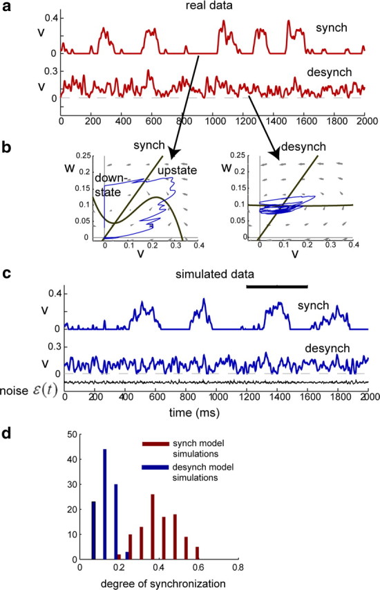
Spontaneous activity simulated via the model. a, Two seconds of real data from synchronized (top) and desynchronized (bottom) states within the same recording session. b, Model fits for the data in a. When the model is fit on the synchronized data (left), the resulting phase diagram is highly nonlinear and consistent with dynamics that alternate between downstates and transient upstates. In contrast, when the model is fit on desynchronized data (right), the resulting phase diagram is nearly linear and reflects a stable baseline firing rate with fluctuations about the mean (fixed point). Trajectories for simulated data (blue) are superimposed on the phase diagrams, taken from the time interval denoted by the black bar in c. c, Using the model fits in b, we generated simulated spontaneous activity by driving each model with noise (see Materials and Methods). The same randomly generated noise input (black) produces very different simulated activity for synchronized and desynchronized model fits; the simulated data qualitatively resembles the real data in a. d, The analysis in c was repeated for 100 randomly generated filtered noise sequences of length 3 s. For each data segment simulated from one of the model fits in b, the degree of synchronization was computed based on the MUA power spectrum, independently of the model parameters (see Materials and Methods). Data segments produced by the model fit to (de)synchronized data consistently exhibited power spectra characteristic of (de)synchronized experimental recordings. synch, Synchronized; desynch, desynchronized.

Generating simulated data from the model.

Simulated data can be generated from the model for a given time series of “kicks” {ε(t)} by simply evolving the model equations (for a fixed set of parameters) with ε(t) as a driving force input at each time t. We have done this in two situations: (1) to generate simulated spontaneous activity data, as in Figure 4 and supplemental Figure 5 (available at www.jneurosci.org as supplemental material), and (2) to generate simulated stimulus-evoked activity, as in Figures 5 and 6. Note that v is allowed to go negative when we integrate the FHN equations; for comparison with experimental data, we later threshold the values [v]₊ so that negative values are replaced with 0.

Figure 5.

Stimulus-evoked activity simulated using the model. a, Evoked responses were simulated by driving the models of Figure 4 with an α-function kick driving force ε(t) starting from different activity states at time t = 0 (colored dots). b, Time-domain representation. Simulated responses in the synchronized state are highly sensitive to activity state at the time of the stimulus and exhibit stimulus-evoked flips: up–down and down–up transitions. In the desynchronized state, simulated responses are more stereotyped and less dependent on initial conditions. c, Same as in b, but each response is generated from a noisy driving force ε(t) (bottom black trace), obtained by adding noise as in Figure 4 to the kick in (a, b). synch, Synchronized; desynch, desynchronized.

Figure 6.

Stimulus-evoked responses can be predicted from models fit on prior spontaneous activity. a, Methodology. Three seconds of spontaneous activity preceding the stimulus is used to fit the model parameters. The model-fit dynamic state (illustrated by the corresponding phase diagram), together with the activity state at the time of the stimulus (green asterisk), is then used to simulate an evoked response (blue), shown superimposed on the true response (red). As in Figure 1, time 0 corresponds to presentation of click stimulus, and shaded regions correspond to initial (dark gray) and persistent (light gray) response periods. b, c, Estimated dynamic states and simulated responses for each trial displayed in Figure 1. d, Prediction error for a single trial from rat 1 (red line), compared with predictions for the response on this trial made from states estimated for all other trials. Estimates from other trials, both within the same recording (left) and from other recordings (right), produced worse predictions. e, Box plots of model-fit percentiles for each trial, within and across recordings. Median percentiles (red) are, in each case, significantly above chance level (50%). f, Same as in e, but performance is compared using only dynamic states from other trials, keeping activity state at stimulus onset fixed. For recording sessions with high cortical state variability (1 and 2), percentiles were still high within and across recordings. For recording sessions with a very stable dynamic state (3 and 4), percentiles were not significantly above chance within each recording but remained high across recordings.

In situation 1, we obtained a “noise” time series ε(t) by first sampling independently from a lognormal distribution (with a mean of 25 and variance of 100) and then filtering the resulting white noise time series so that its power spectrum matched that of the residuals obtained when the model was fit on desynchronized data. Residuals of desynchronized rather than synchronized data were used for the power spectrum because the residuals from synchronized data cannot be accurately determined during downstates, as the thresholded values of v match the data exactly during these periods. A lognormal distribution was used as the residuals had heavier tails than a Gaussian, to which the lognormal distribution allowed a good approximation.

In situation 2, stimulus-evoked responses were simulated by evolving the model according to initial conditions (v₀, w₀) at the time of the stimulus and an α-function ε(t) (to simulate the stimulus) given by the formula ε(t) = α(t − t₀)e^{(t₀ − t)/β}. The parameters t₀, α, and β were chosen to be constant on an experiment-wide basis, reflecting repeated presentations of loud noise-click stimuli within the same recording. In Figure 6b (rat 3), we had t₀ = 10 ms, h = 0.018, β = 5 ms, and α = 0.0036e ms⁻¹, where h = αβ/e is the maximum height of the α-function. In Figure 6c (rat 1), we had t₀ = 10 ms, h = 0.021, β = 6 ms, and α = 0.0035e ms⁻¹.

Evaluating the performance of the model.

To measure the performance of the model on any given trial, we first fit the parameters of the model on the 3 s of spontaneous activity data immediately preceding the stimulus. The performance of the model in predicting the structure of the subsequent response was then quantified as follows. Using Equation 1 together with the time series {v(t), w(t)} for the first 300 ms of the response period, we derived the error term ε(t) that would be required at each time step as a driving force in order for the model, with the given parameters, to exactly reproduce the stimulus-evoked response. The “prediction error” for the model in predicting this response is then defined as _T̄¹∫ε²(t)dt, where T = 300 ms is the length of the response period. Note that the prediction error does not depend on comparison with a particular simulated response; rather, it is a measure of how naturally the real response trajectory follows the flow lines of the model's phase diagram. To compute the “fit error” (supplemental Fig. 8, available at www.jneurosci.org as supplemental material), the same metric was used with ε(t) obtained as the residuals from fitting the model to spontaneous activity data.

Quantitative assessment of model characteristics.

To assess the linearity of a particular fit model f(v, w), we obtained the model's linear approximation f_lin(v, w) from the Jacobian evaluated at the fixed point closest to the origin (usually there is only one fixed point). We define the “degree of nonlinearity” to be the log of the normalized norm of the difference

and the integral is computed on a fine grid. (Note that almost all of the data is confined to the region [0,0.4]×[0,0.25] of the v − w plane.)

To quantify the variability of dynamic state throughout a recording, we computed the summed point-wise variance

of the vector fields f(v, w) computed over all model fits (one for each sensory stimulus) in a given recording.

Results

We recorded populations of 50–100 cells, together with LFPs, from auditory cortex of urethane-anesthetized rats using silicon microelectrodes (see Materials and Methods). We recorded both spontaneous and click-evoked activity across a range of synchronized and desynchronized states and focused our analysis on smoothed MUA obtained by pooling together all spikes from simultaneously recorded neurons (see Materials and Methods).

We began by visualizing how click responses vary with cortical state. In the neocortex, the word “state” is used with two different meanings, corresponding to two different time scales. We shall refer to the state of the cortex, in the sense of the dynamics of network activity on a time scale of seconds or more and as reflected in the LFP power spectrum, as its “dynamic state”; the synchronized and desynchronized states are examples of dynamic states. The word “state” is also used to refer to fluctuations in instantaneous network activity at time scales of the order hundreds of milliseconds, as in the case of upstates and downstates. We will use the term “activity state” to describe cortical states that persist on these shorter time scales.

To illustrate how sensory responses can depend on activity state at the time of stimulus presentation, Figure 1a shows population activity before and after six presentations of a click stimulus in a recording that was consistently in the synchronized state. It has been reported that in somatosensory cortex, whisker stimulation can “flip” neural activity from downstate to upstate and vice versa (Hasenstaub et al., 2007). Visual examination of our data suggested that click stimuli presented during the synchronized state can evoke a similar flip in auditory cortex. When the stimulus arrived during a downstate, an upstate frequently ensued (Fig. 1a, trials 1 and 2). Similarly, stimuli that arrived during upstates could trigger downstates (Fig. 1a, trials 5 and 6). Note that the initial response to the click (10–35 ms; dark gray shading) was approximately similar across trials, whereas the persistent response (40–135 ms; light gray shading) was more strongly modulated by ongoing cortical activity at the time of the stimulus.

Figure 1.

Trial-to-trial variability across a range of cortical states. a, Six examples of population responses to click stimuli, from a rat that exhibited stable dynamic state throughout the recording. Vertical green lines denote stimuli (time 0); LFP (black trace), activity of simultaneously recorded single neurons (rasters), and smoothed MUA (red trace) all show a pattern of population activity characteristic of the synchronized state. The right column shows an expanded view of the smoothed MUA in the response period for each trial; gray shaded areas denote “initial” (10–35 ms; dark gray shading) and “persistent” (40–135 ms; light gray shading) response periods. The stimulus may arrive during a downstate (trials 1 and 2), at the beginning of an upstate (trials 3 and 4), or well into an upstate (trials 5 and 6). Whereas preceding activity does not have a clear effect on peak activity levels in the initial response period, the timing of the stimulus relative to up/down transitions appears to modulate activity in the persistent response period. b, Same conventions as in a; all data are selected from a different recording session that showed variable dynamic state. In the synchronized (synch) state (trials 1 and 2), persistent responses are anticorrelated with activity levels in the 200–300 ms preceding the stimulus. In intermediate states (trials 3 and 4), the stimulus induces a large initial response followed by a transient downstate. In the most desynchronized (desynch) states (trials 5 and 6), responses exhibit a small but reliable initial response followed by a return to baseline, with no discernible persistent response.

To illustrate how dynamic state can affect click responses, Figure 1b shows data from a recording session whose dynamic state spontaneously varied from highly synchronized (trials 1 and 2) to highly desynchronized (trials 5 and 6) activity. In these data, synchronized and desynchronized are not discrete cortical states but, rather, extremes in a continuum. In the more synchronized cases (Fig. 1b, top), responses follow a pattern similar to that shown in Figure 1a. In desynchronized states, however (Fig. 1b, bottom), the persistent response appears to be weakly modulated by the stimulus, instead returning to a baseline firing rate that matches the average firing rate preceding the stimulus.

Persistent activity (anti-)correlates with past activity in a state-dependent manner

To quantify the above observations, we began with a correlational analysis. We define two “mean field” variables, v and w, that summarize activity state at each instant (see Materials and Methods). The variable v measures average population firing rate and is represented by the red trace in Figure 1 and throughout the paper. The variable w measures the integrated recent activity of the network and is obtained by convolving v with a causal, decaying exponential filter of time constant τ = 100 ms (i.e., passing v through a leaky integrator) (Fig. 2a). This value of τ was chosen to maximize the (anti-)correlation of w with persistent responses (see below).

To examine how sensory responses depend on the combination of dynamic state and activity state, we divided the trials into five dynamic state categories ranging from the most synchronized to the most desynchronized, based on the fraction of 0–50 Hz power that comes from the 0–5 Hz interval (see Materials and Methods). Figure 2b shows a raster representation of population responses to clicks for each of these dynamic state categories, accumulated across all recordings (a similar analysis for each recording separately is shown in supplemental Fig. 1, available at www.jneurosci.org as supplemental material). Within each plot, trials are further sorted by the value of w at the time of stimulus presentation. Examination of plots corresponding to the most synchronized states (Fig. 2b, top) agreed with the visual impression conveyed by Figure 1a, indicating that click stimuli could flip upstates and downstates and that activity state at the time of click presentation had more effect on persistent responses than on initial responses. For lower levels of synchronization (Fig. 2b, middle), the effect of prior activity state on persistent responses decreased. In the most desynchronized trials (Fig. 2b, bottom), there did not appear to be a clear persistent response.

Figure 2, c and d, shows, for each dynamic state category, the correlation of initial (10–35 ms) and persistent (40–135 ms) firing rate responses with the normalized past activity w at the time of stimulus presentation. As expected, robust negative correlations were seen between past activity and persistent response periods in synchronized states (Fig. 2c,d, top). This negative correlation did not simply reflect the tendency of upstates and downstates to alternate in the absence of sensory stimuli, as confirmed by its absence in control analyses centered on randomly chosen times when no stimulus was presented (phantom trials) (supplemental Figs. 2–4, available at www.jneurosci.org as supplemental material). For more desynchronized states, the negative correlation was less pronounced. For the most desynchronized states (Fig. 2c,d, bottom) a positive correlation was seen, although this did not reflect a true persistent response but, rather, a return to the prestimulus baseline, as evidenced by a similar positive correlation in the phantom trial data (supplemental Figs. 2–4, available at www.jneurosci.org as supplemental material). The initial response period showed a smaller modulation by prior activity than the persistent period, with a strong negative correlation seen only in the most synchronized states.

A simple model of cortical state

The previous results (Fig. 2) indicate a complex dependence of sensory responses on dynamic and activity states at the time of stimulus presentation. We now aim to show that this apparently complex relationship can be explained by a simple principle: sensory responses are shaped by the same dynamics that generate spontaneous activity before stimulus presentation. We will do this by showing that a dynamical system model, with parameters estimated from spontaneous activity preceding a stimulus, can quantitatively predict the subsequent sensory response.

Because dynamic state can vary over a time scale of several seconds, to gain an accurate “snapshot” of ongoing dynamics we will need to estimate model parameters from segments of only a few seconds of data. We found that a simple family of self-exciting dynamical systems yields good approximations for the different dynamic states observed in our data. There are many families of self-exciting system models (Izhikevich, 2007). We have chosen the FHN equations (Fitzhugh, 1955), as they are of simple form, are sufficiently flexible to allow a wide range of linear and nonlinear dynamics (supplemental Fig. 5, available at www.jneurosci.org as supplemental material), and allow rapid and robust parameter estimation from as little as 3 s of MUA data (Fig. 3). Although in neuroscience these equations are usually considered as models for action potential generation in single neurons, they offer flexibility to model a wide range of self-exciting systems. The equations (identified previously as Eqs. 1 and 2) are as follows:

In this scheme, the dynamical variables v(t) and w(t) correspond to the activity state of the network at any instant, whereas the model parameters (a₁, a_2, a_3, b, and I) that specify how v and w evolve in time correspond to its dynamic state. In our case, v represents the mean firing rate of cortical neurons and is estimated by the smoothed MUA as described above. Because v may, at times, be negative in data simulated using the model, the final output is thresholded as [v]₊ = max (v, 0) when comparing with observed population firing rates (see Materials and Methods); note that this does not affect the temporal evolution of (v, w) dictated by the equations. The variable w, as can be seen from Equation 2, corresponds to the integrated past activity variable previously defined. It is because Equation 2 allows us to compute w directly from v, independent of the parameters in Equation 1, that we are able to rapidly fit the parameters of the FHN model. After computing w, the parameters in Equation 1 can be fit using linear regression, thus avoiding more computationally intensive methods that would, in general, be needed for fitting the parameters of a set of coupled differential equations. The term ε(t) represents inputs driving v that are external to the model, such as noise or stimulus-driven inputs. The model is fit by minimization of ε²(t) on periods of spontaneous activity (see Materials and Methods).

Although for our purposes this is a phenomenological model, we note that its functional form can also be interpreted mechanistically as a model of mean field network dynamics, in which the mean rates of excitatory and inhibitory cells are both proportional to v and w represents the combined effects of adaptive phenomena such as synaptic depression and cellular accommodation that reduce network excitability. In this scheme, the coefficients of the model can also be given mechanistic interpretations (Fig. 3c), with a₁, a₂, and a₃ corresponding to recurrent excitation and inhibition; b determining the extent to which increases in w reduce the excitability of the network; and I representing a constant “tonic drive” on all cells, such as might arise from an increase in mean thalamic firing rates, or neuromodulatory activity that promotes tonic firing.

Once the parameters have been fit, the dynamics of the resulting model can be visualized using the “phase portrait,” a common tool of dynamical systems theory (Izhikevich, 2007). The phase portrait is a two-dimensional plot corresponding to the possible values of v and w, on which is displayed a vector field showing how a system in a state (v, w) will evolve with time according to Equations 1 and 2, and “nullclines,” curves along which one of the equations is 0 (i.e., one of the variables does not change in time). Fixed points occur where the two nullclines intersect. Some examples of possible phase portraits for the FHN equations are shown in supplemental Figure 5 (available at www.jneurosci.org as supplemental material), together with examples of their dynamics. We note that in a deterministic dynamical system, in which the driving term ε(t) is 0, the qualitative behavior of the system is determined by the topology of the phase portrait. However, in a stochastic system (i.e., one driven by external noise), changes in phase portrait topology do not correspond to sudden shifts in the qualitative behavior of the system. We may therefore see similar behavior for similar values of model parameters, even if they have topologically distinct phase portraits (supplemental Fig. 5, rows 1–4, available at www.jneurosci.org as supplemental material), as well as different behavior for models having the same phase portrait topology (supplemental Fig. 5, rows 4–5, available at www.jneurosci.org as supplemental material).

Model captures qualitative features of spontaneous and sensory evoked activity

To verify that the model-fitting procedure can indeed capture the dynamics underlying spontaneous activity in synchronized and desynchronized states, we first examined simulated spontaneous activity. We fit the model to 3 s segments of spontaneous activity in the synchronized and desynchronized states (Fig. 4a), obtaining parameters (a₁, a₂, a₃, b, I) in each case (Fig. 4b) (see Materials and Methods for actual values of the parameters in this case). We then simulated spontaneous activity by driving the model with filtered noise ε(t) (see Materials and Methods). Although exactly the same noise sequence was used in both cases, the resulting simulated activity was strikingly different and closely mimicked the structure of the original data segments used to fit the models (Fig. 4c). To statistically confirm this observation, we repeated this procedure for 100 randomly generated traces of filtered noise ε(t), in each case using the same noise sequence to simulate 3 s of data for both models in Figure 4b. We then computed the degree of synchronization for each simulated data segment using the power spectrum measure defined above (see Materials and Methods). Data simulated from the two models showed a clear difference in the degree of synchronization, confirming that noise-driven models fit from spontaneous activity are capable of capturing this difference in the original data.

We next asked whether the dynamics estimated by this procedure can account for the qualitative structure of stimulus-evoked responses. To do this, we used an α-function kick for ε(t) to drive the model in a way that mimics the effect of a click stimulus (Fig. 5) (see Materials and Methods). In the synchronized state, simulated sensory responses varied greatly depending on the activity state at the time of the stimulus; the pattern of variability was qualitatively similar to that observed in the real data, with simulated responses exhibiting both down–up and up–down state flips (Fig. 5a,b, top row), despite being generated with identical model parameters and an identical kick driving force ε(t). In the desynchronized state, response variability was greatly diminished; regardless of activity state at the time of the stimulus, all responses exhibited an initial positive deflection followed by a brief suppression of activity (Fig. 5a,b, bottom row). In both synchronized and desynchronized states, the basic pattern of simulated responses was preserved in the presence of added noise (Fig. 5c).

Model quantitatively predicts the structure of stimulus-evoked responses

The above analyses show that models estimated from spontaneous activity can capture qualitative features of cortical dynamics in synchronized and desynchronized states. We next asked whether these models can also quantitatively predict actual sensory responses on a trial-by-trial basis. To investigate this, we tested whether models fit on a short period (∼3 s) of spontaneous activity immediately preceding a stimulus were able to predict the structure of activity in the subsequent sensory response.

The prediction methodology is illustrated in Figure 6a. A model fit from spontaneous activity preceding a stimulus yields an estimate of cortical state, including dynamic state (captured by model parameters a₁, a₂, a₃, b, and I) (Fig. 6a, phase portrait) and activity state (v and w) (Fig. 6a, green asterisk) at the time of the stimulus. A predicted response can be generated by solving the model equations with the fit parameters, using initial conditions given by the activity state, and driven by an α-function driving force ε(t) without noise (Fig. 6a, right). Figure 6b shows model-based estimates of cortical state and predicted responses for each of the trials displayed in Figure 1a (left column). Visual inspection suggested that predicted responses (blue) typically closely matched actual responses (red) for a period of 100–200 ms after click presentation. Later features of the response, such as “rebounds” from downstates that sometimes occurred ∼200 ms after click onset, were predicted with less accuracy. Because these trials all had a similar dynamic state, there was relatively little variation in the model-fit phase portraits, and response variability was primarily explained by differences in activity state (Fig. 6b, green asterisks) at the time of the stimulus. Figure 6c shows the predictions of the model for the trials in Figure 1b, in which both dynamic and activity state were variable. Again, the model typically predicted the early component of the response well, with accuracy decaying after a period of 100–200 ms. Model fits were not perfect: one feature that the model erroneously predicted was an induced suppression at ∼100 ms in the most desynchronized trials (Fig. 6c, bottom row). Nevertheless, despite its simplicity, the model appeared to capture the major features of cortical population responses across a range of dynamic states.

We next quantified the ability of the models fit on each trial to predict the structure of the subsequent evoked response. Because small differences in the driving force ε(t) attributable to the presence of noise may lead to large changes in the response trajectory, time-domain comparison of actual responses to particular predicted responses may be misleading. Instead, we used an approach that directly compares actual responses to the dynamics predicted by the model. To do this, we first computed the driving force ε(t) that would be necessary for the model to produce the observed response in the 300 ms following the time of the stimulus (see Materials and Methods). The integral of ε²(t) was used as a measure of how hard the model would have to be driven to exactly match the data; we call this the prediction error. The smaller the prediction error, the more naturally the real response trajectory follows the flow lines in the model's phase diagram. Thus, if responses evolve according to the same cortical dynamics that govern the preceding spontaneous activity, and the model parameters capture these dynamics, then a model estimated from spontaneous activity preceding a given stimulus should outperform control models fit from other periods.

To assess performance, we compared the prediction error of the model fit on spontaneous activity before a given trial with the prediction errors of a null ensemble of models derived from other stimulus presentations; this enabled us to assign a percentile to each trial compared with the null ensemble (Fig. 6d). By comparing to various null ensembles, we were thus able to test various hypotheses for the model's ability to capture the role of activity state and dynamic state in shaping click responses. We first used a null ensemble of models fit to spontaneous activity before all other click presentations, either within the same recording session or in all other recording sessions (Fig. 6e). In this analysis, both activity state and dynamic state from alternative trials were used to determine the distribution of comparison prediction errors. Use of the correct model gave better performance than these ensembles, verifying that the model was able to capture the combined effects of activity and dynamic state on click responses.

We next asked whether the model could capture response variability attributable to differences in dynamic state alone. To assess this, we used a null ensemble in which dynamic states were fit from other trials, but activity state was always obtained from the correct trial. We hypothesized that in recordings with stable dynamic state, prediction errors of this ensemble should not differ significantly from the prediction error of the model corresponding to the correct trial, but in recordings with variable dynamic state, the model from the correct trial should perform better. In two of the four experiments (rats 3 and 4), dynamic state was stable, whereas in two others (rats 1 and 2) it varied throughout the recording. (Dynamic state variability was quantified by the variance of the associated vector fields, with variances of 2.05, 3.27, 0.04, and 0.23 for rats 1–4, respectively; see Materials and Methods.) As expected, model predictions in recording sessions with low dynamic state variability did not display significantly better prediction than the ensemble, but higher performance was observed in recordings with variable dynamic state (Fig. 6f, left). When using a null ensemble derived from dynamic states for trials in other recording sessions, performance was better in every case (Fig. 6f, right). Pairwise comparisons between rats exhibited the same pattern as seen in Figure 6, e and f, and supplemental Fig. 6 (available at www.jneurosci.org as supplemental material).

Models fit to the desynchronized state are close to linear

The above analyses show that a simple, low-dimensional model of cortical dynamics can explain many aspects of the variability and state dependence of auditory cortical sensory responses. We next used the model to investigate the character of the dynamics in different states. Figure 7 shows an illustrative segment of data recorded from rat 1 after click presentations had finished, in which desynchronization was repeatedly evoked by stimulation of the PPT (supplemental Fig. 7, available at www.jneurosci.org as supplemental material). PPT stimulation induced rapid desynchronization, after which activity slowly returned to a synchronized state. Models fit to successive 3 s intervals of spontaneous activity data between PPT stimulations showed gradual changes (Fig. 7a), with the locations of fixed points in each model phase diagram tracking the slow evolution of cortical dynamics from desynchronized to synchronized states. Examination of phase portraits suggested that models fit during the synchronized state were highly nonlinear, whereas those during desynchronized states immediately after PPT stimulation corresponded to approximately linear vector fields (Fig. 7b).

Figure 7.

Models fit to the desynchronized state are more linear than to the synchronized state. a, Evolution of states for a segment of 135 s of continuous spontaneous activity in which desynchronization was induced with electrical stimulation of the PPT (pink vertical bars). Data were subdivided into 45 adjacent, nonoverlapping 3 s intervals. For each interval, the model was fit, and a phase diagram was obtained. The location of the fixed point along the v-axis of the phase diagram is plotted for each interval (dark blue dots) and closely follows the mean firing rate (green trace). After each PPT stimulation, cortical activity undergoes a sharp transition to the desynchronized state, followed by a gradual decay over tens of seconds back to the synchronized state. b, Sample phase diagrams corresponding to shaded 3 s intervals in a. Before PPT stimulation, the cortex was in a synchronized state, with a highly nonlinear phase diagram (i). Immediately after PPT stimulation, near-linear dynamics are seen (ii) that gradually become more nonlinear as the cortical state returns to synchronization (iii, iv). c, Degree of synchronization versus degree of nonlinearity for nonoverlapping 3 s spontaneous activity periods of one recording. Degree of synchronization is computed from the power spectrum; degree of nonlinearity measures the nonlinearity of the vector field corresponding to each model fit (see Materials and Methods). d, A similar correlation can be seen in data pooled from all recording sessions. deg, Degree; synch, synchronized; desynch, desynchronized.

To verify statistically that modeled dynamics were closer to linear in more desynchronized states, we computed a measure of model linearity and a measure of synchronization derived independently of the model using the power spectrum (see Materials and Methods for details of linearity and synchronization measures; the same synchronization measure was used to define the synchronization ranges in Fig. 2). Figure 7, c and d, shows the relationship between these two measures for a single recording session and for all recordings pooled, respectively. The accuracy with which the model fit spontaneous data did not show a clear correlation with dynamic state (supplemental Fig. 8, available at www.jneurosci.org as supplemental material). However, a strong correlation was observed between dynamic state and model linearity in both cases. Thus, models fit to desynchronized data are consistently more linear than models fit to synchronized data, with a full spectrum of dynamics between the two extremes.

Discussion

Population responses to click stimuli in urethane-anesthetized auditory cortex were complex and state dependent. However, the structure of these responses could be quantitatively predicted on a trial-to-trial basis using a simple, low-dimensional dynamical system model, with parameters estimated from spontaneous activity preceding each stimulus. Optimal prediction of sensory responses required estimating both activity state (population rate at the time of stimulus presentation and integrated over the previous several hundred milliseconds) and dynamic state (model parameters fit from the previous 3 s of spontaneous activity). Analysis of model fits indicated that dynamics in synchronized states can be approximated by a self-exciting system, whereas desynchronized states were better approximated by a linear model.

Cortical circuits contain large numbers of neurons of diverse physiology, intricately connected by synapses that themselves exhibit complex dynamics. Large and complex systems are studied in many fields of science; in some cases, the collective behavior of such systems can be described by emergent low-dimensional dynamics. In models of physical systems, this is often achieved by mean field approximation, an approach also used in neural network models (Mezard et al., 1987; Amit, 1989), including models of upstates and downstates in cortical circuits (Holcman and Tsodyks, 2006). We found that the activity of auditory cortical populations could be approximated by a simple dynamical system model, suggesting that, at least for the system we studied, collective cortical dynamics do have an effective low-dimensional description.

We used the FHN equations to model cortical dynamics because they allow tractable parameter fitting from short data segments. Although these equations can be interpreted in terms of cortical circuitry (Fig. 3c), no attempt was made to match the model structure to known details of cortical physiology. Nevertheless, our phenomenological model can be fit directly to data and may thus help bridge the gap between large-scale population recordings and more detailed, biophysically inspired network models (Bazhenov et al., 2002; Compte et al., 2003; Soto et al., 2006; Loebel et al., 2007; Parga and Abbott, 2007; Izhikevich and Edelman, 2008). The model provided a good approximation to the observed data in a wide range of circumstances, but model fits were not perfect. First, although predicted and actual responses matched closely for early sensory responses, they progressively diverged after click presentation. We suggest this did not result specifically from the FHN model but would occur in whatever model family was used. In a noise-driven dynamical system, two trajectories from the same initial conditions will diverge with time; furthermore, although the FHN system we considered is not (deterministically) chaotic, nonlinearities will likely amplify this divergence. A second inaccuracy we found was more specific: when fit to desynchronized data, the model predicted a suppression of spiking activity ∼100 ms after click presentation. Such suppression was frequently seen in desynchronized states but not in the very most desynchronized trials. Intriguingly, previous work shows that in the desynchronized cortex of awake rats, the ability of transcallosal stimulation to induce a similar period of suppression depends on the animal's precise behavior (Vanderwolf et al., 1987; Dringenberg and Vanderwolf, 1994). A more accurate model than FHN might be able to distinguish these subdivisions within the desynchronized state.

Despite the likely suboptimality of the FHN system, the models fit with these equations suggest a qualitative picture of collective cortical dynamics that may be independent of the particular model family used. In synchronized states, dynamics were modeled by a self-exciting system, which can explain stimulus-induced flipping of upstates and downstates. According to the suggested interpretation of the model, self-excitation arises from recurrent excitation within cortex, counterbalanced by a build-up of adaptive processes such as synaptic depression and potassium channel activation, modeled by the w parameter. In downstates, w is small, and sensory stimulation triggers a rapid increase in v because of self-excitation. This leads to prolonged activity (an upstate), until w has increased enough to damp down the network's excitability. When stimuli are presented in an upstate, however, v is initially high and w is of intermediate value, not yet enough to terminate the upstate. In this case, sensory stimulation causes a transient increase in v, followed by an increase in w, which accelerates transition back to the downstate. We note that models fit to the synchronized state typically showed only a single stable fixed point corresponding to the downstate, with the upstate represented instead by a close approach of nullclines. In stochastic dynamical systems, however, differing topologies of phase portraits do not necessarily indicate qualitative changes in the noise-driven dynamics (supplemental Fig. 5, available at www.jneurosci.org as supplemental material). The fact that upstates do not correspond to fixed points likely reflects the fact that auditory cortical upstates are of short duration (cf. DeWeese and Zador, 2006). During desynchronized states, model fits were close to linear, with a single stable fixed point at intermediate values of v and w. In this state, stimuli caused reliable transient perturbations of both v and w, corresponding to the lower trial-to-trial variability seen in this state. A combination of recurrent excitation and network adaptation, with dynamics that vary with cortical state, may thus explain several features of cortical population dynamics. We note that a recent network model based on recurrent excitation and synaptic depression was also able to reproduce features of auditory cortical responses to several stimulus paradigms (Loebel et al., 2007).

The nonlinear interaction of sensory responses and ongoing activity during the synchronized state is consistent with observations in somatosensory cortex (Hasenstaub et al., 2007) but might at first appear to contradict findings in cat visual cortex (Arieli et al., 1996), which suggested that trial-to-trial variability could be modeled by linear summation of a stereotyped response onto otherwise unchanged background activity. Although our results suggest that dynamics in the desynchronized state are approximately linear, it is unlikely that desynchronization led to linear summation in the study by Arieli et al. (1996), as these experiments were performed under deep barbiturate anesthesia. A more likely scenario is that linear summation resulted from focusing on an initial (50 ms) response period, which we found exhibits smaller nonlinear state-dependent dynamics than the persistent response period.

Because our results were collected under urethane anesthesia, a natural question concerns whether the awake cortex would behave similarly. Although it was originally believed that the awake cortex is in a uniform desynchronized state, recent results show that cortical populations in awake resting rats show coordinated fluctuations in firing rate, which correlate with the LFP (Luczak et al., 2007, 2009; Poulet and Petersen, 2008). LFP power spectra show variations within awake animals, changing with factors such as attention (Fries et al., 2001b), suggesting that the dynamics of population rate fluctuations can vary with behavioral and cognitive state. Furthermore, stimulus responses vary with behavior and with the phase of ongoing oscillations in awake subjects (Vanderwolf et al., 1987; Dringenberg and Vanderwolf, 1994; Fries et al., 2001a; Lakatos et al., 2008). Population dynamics may thus play a key role in shaping the responses of the awake cortex to sensory stimuli. Our results suggest that under urethane, the dynamics of both spontaneous fluctuations and sensory responses can be approximated by a low-dimensional model; similar methods could determine whether the same holds for population dynamics in awake animals.

What mechanisms might account for the differences in cortical dynamics between states? The activity of ascending neuromodulatory systems correlates with brain state (Duque et al., 2000; Manns et al., 2000; Portas et al., 2000; Berridge and Waterhouse, 2003), causing multiple changes in the dynamics of individual cells and synapses and thus in the dynamics of thalamocortical networks (Metherate et al., 1992; McCormick et al., 1993; Gil et al., 1997; McCormick and Bal, 1997; Steriade et al., 2001; Bazhenov et al., 2002). Several neuromodulatory effects may contribute to linearization of cortical dynamics, including inhibition of recurrent excitatory connections (Gil et al., 1997; Hasselmo, 1999), reduction of cellular nonlinearities (Nicoll, 1988), and promotion of tonic firing (Wang and McCormick, 1993; Hasselmo, 1995; Beierlein et al., 2002). One of the clearest features of models fit to desynchronized data was an increase in the tonic drive parameter I, resulting in a fixed point at high values of v and w. We note that desynchronized states are characterized by increased baseline firing rates in the thalamus (Castro-Alamancos and Oldford, 2002) and that neuromodulators may cause tonic inward currents in cortical pyramidal cells (Wang and McCormick, 1993), providing a possible physiological interpretation of the I parameter. Linearity of dynamics in the desynchronized state could allow the cortex to faithfully represent afferent sensory stimuli; in contrast, nonlinear dynamics in the synchronized state may lead to high trial-to-trial variability, as exemplified by the ability of a stimulus to produce up–down and down–up transitions.

In summary, our results suggest that the apparently complex and state-dependent interaction of sensory responses with ongoing activity can be understood by the simple principle that sensory-evoked responses are shaped by the same dynamics that govern ongoing spontaneous activity. Furthermore, despite the complexity of the underlying neural circuits, population dynamics can be quantitatively modeled in a remarkably simple way, with changes in state corresponding consistently to changes in circuit dynamics.

References

- Amit D. Cambridge, UK: Cambridge UP; 1989. Modeling brain function. [Google Scholar]
- Arieli A, Sterkin A, Grinvald A, Aertsen A. Dynamics of ongoing activity: explanation of the large variability in evoked cortical responses. Science. 1996;273:1868–1871. doi: 10.1126/science.273.5283.1868. [DOI] [PubMed] [Google Scholar]
- Bazhenov M, Timofeev I, Steriade M, Sejnowski TJ. Model of thalamocortical slow-wave sleep oscillations and transitions to activated States. J Neurosci. 2002;22:8691–8704. doi: 10.1523/JNEUROSCI.22-19-08691.2002. [DOI] [PMC free article] [PubMed] [Google Scholar]
- Beierlein M, Fall CP, Rinzel J, Yuste R. Thalamocortical bursts trigger recurrent activity in neocortical networks: layer 4 as a frequency-dependent gate. J Neurosci. 2002;22:9885–9894. doi: 10.1523/JNEUROSCI.22-22-09885.2002. [DOI] [PMC free article] [PubMed] [Google Scholar]
- Berridge CW, Waterhouse BD. The locus coeruleus-noradrenergic system: modulation of behavioral state and state-dependent cognitive processes. Brain Res Brain Res Rev. 2003;42:33–84. doi: 10.1016/s0165-0173(03)00143-7. [DOI] [PubMed] [Google Scholar]
- Castro-Alamancos MA. Absence of rapid sensory adaptation in neocortex during information processing states. Neuron. 2004;41:455–464. doi: 10.1016/s0896-6273(03)00853-5. [DOI] [PubMed] [Google Scholar]
- Castro-Alamancos MA, Oldford E. Cortical sensory suppression during arousal is due to the activity-dependent depression of thalamocortical synapses. J Physiol. 2002;541:319–331. doi: 10.1113/jphysiol.2002.016857. [DOI] [PMC free article] [PubMed] [Google Scholar]
- Clement EA, Richard A, Thwaites M, Ailon J, Peters S, Dickson CT. Cyclic and sleep-like spontaneous alternations of brain state under urethane anaesthesia. PLoS ONE. 2008;3:e2004. doi: 10.1371/journal.pone.0002004. [DOI] [PMC free article] [PubMed] [Google Scholar]
- Compte A, Sanchez-Vives MV, McCormick DA, Wang XJ. Cellular and network mechanisms of slow oscillatory activity (<1 Hz) and wave propagations in a cortical network model. J Neurophysiol. 2003;89:2707–2725. doi: 10.1152/jn.00845.2002. [DOI] [PubMed] [Google Scholar]
- DeWeese MR, Zador AM. Shared and private variability in the auditory cortex. J Neurophysiol. 2004;92:1840–1855. doi: 10.1152/jn.00197.2004. [DOI] [PubMed] [Google Scholar]
- DeWeese MR, Zador AM. Non-Gaussian membrane potential dynamics imply sparse, synchronous activity in auditory cortex. J Neurosci. 2006;26:12206–12218. doi: 10.1523/JNEUROSCI.2813-06.2006. [DOI] [PMC free article] [PubMed] [Google Scholar]
- Doron NN, LeDoux JE, Semple MN. Redefining the tonotopic core of rat auditory cortex: physiological evidence for a posterior field. J Comp Neurol. 2002;453:345–360. doi: 10.1002/cne.10412. [DOI] [PubMed] [Google Scholar]
- Dringenberg HC, Vanderwolf CH. Transcallosal evoked potentials: behavior-dependent modulation by muscarinic and serotonergic receptors. Brain Res Bull. 1994;34:555–562. doi: 10.1016/0361-9230(94)90140-6. [DOI] [PubMed] [Google Scholar]
- Duque A, Balatoni B, Detari L, Zaborszky L. EEG correlation of the discharge properties of identified neurons in the basal forebrain. J Neurophysiol. 2000;84:1627–1635. doi: 10.1152/jn.2000.84.3.1627. [DOI] [PubMed] [Google Scholar]
- Edeline JM. The thalamo-cortical auditory receptive fields: regulation by the states of vigilance, learning and the neuromodulatory systems. Exp Brain Res. 2003;153:554–572. doi: 10.1007/s00221-003-1608-0. [DOI] [PubMed] [Google Scholar]
- Faisal AA, Selen LP, Wolpert DM. Noise in the nervous system. Nat Rev Neurosci. 2008;9:292–303. doi: 10.1038/nrn2258. [DOI] [PMC free article] [PubMed] [Google Scholar]
- Fitzhugh R. Mathematical models of threshold phenomena in the nerve membrane. Bull Math Biophys. 1955;17:257–278. [Google Scholar]
- Fries P, Neuenschwander S, Engel AK, Goebel R, Singer W. Rapid feature selective neuronal synchronization through correlated latency shifting. Nat Neurosci. 2001a;4:194–200. doi: 10.1038/84032. [DOI] [PubMed] [Google Scholar]
- Fries P, Reynolds JH, Rorie AE, Desimone R. Modulation of oscillatory neuronal synchronization by selective visual attention. Science. 2001b;291:1560–1563. doi: 10.1126/science.1055465. [DOI] [PubMed] [Google Scholar]
- Gil Z, Connors BW, Amitai Y. Differential regulation of neocortical synapses by neuromodulators and activity. Neuron. 1997;19:679–686. doi: 10.1016/s0896-6273(00)80380-3. [DOI] [PubMed] [Google Scholar]
- Haider B, Duque A, Hasenstaub AR, Yu Y, McCormick DA. Enhancement of visual responsiveness by spontaneous local network activity in vivo. J Neurophysiol. 2007;97:4186–4202. doi: 10.1152/jn.01114.2006. [DOI] [PubMed] [Google Scholar]
- Harris KD. Neural signatures of cell assembly organization. Nat Rev Neurosci. 2005;6:399–407. doi: 10.1038/nrn1669. [DOI] [PubMed] [Google Scholar]
- Harris KD, Henze DA, Csicsvari J, Hirase H, Buzsaki G. Accuracy of tetrode spike separation as determined by simultaneous intracellular and extracellular measurements. J Neurophysiol. 2000;84:401–414. doi: 10.1152/jn.2000.84.1.401. [DOI] [PubMed] [Google Scholar]
- Hasenstaub A, Sachdev RN, McCormick DA. State changes rapidly modulate cortical neuronal responsiveness. J Neurosci. 2007;27:9607–9622. doi: 10.1523/JNEUROSCI.2184-07.2007. [DOI] [PMC free article] [PubMed] [Google Scholar]
- Haslinger R, Ulbert I, Moore CI, Brown EN, Devor A. Analysis of LFP phase predicts sensory response of barrel cortex. J Neurophysiol. 2006;96:1658–1663. doi: 10.1152/jn.01288.2005. [DOI] [PubMed] [Google Scholar]
- Hasselmo ME. Neuromodulation and cortical function: modeling the physiological basis of behavior. Behav Brain Res. 1995;67:1–27. doi: 10.1016/0166-4328(94)00113-t. [DOI] [PubMed] [Google Scholar]
- Hasselmo ME. Neuromodulation: acetylcholine and memory consolidation. Trends Cogn Sci. 1999;3:351–359. doi: 10.1016/s1364-6613(99)01365-0. [DOI] [PubMed] [Google Scholar]
- Hentschke H, Haiss F, Schwarz C. Central signals rapidly switch tactile processing in rat barrel cortex during whisker movements. Cereb Cortex. 2006;16:1142–1156. doi: 10.1093/cercor/bhj056. [DOI] [PubMed] [Google Scholar]
- Holcman D, Tsodyks M. The emergence of up and down states in cortical networks. PLoS Comput Biol. 2006;2:e23. doi: 10.1371/journal.pcbi.0020023. [DOI] [PMC free article] [PubMed] [Google Scholar]
- Izhikevich EM. Cambridge, MA: MIT; 2007. Dynamical systems in neuroscience the geometry of excitability and bursting. [Google Scholar]
- Izhikevich EM, Edelman GM. Large-scale model of mammalian thalamocortical systems. Proc Natl Acad Sci U S A. 2008;105:3593–3598. doi: 10.1073/pnas.0712231105. [DOI] [PMC free article] [PubMed] [Google Scholar]
- Kenet T, Bibitchkov D, Tsodyks M, Grinvald A, Arieli A. Spontaneously emerging cortical representations of visual attributes. Nature. 2003;425:954–956. doi: 10.1038/nature02078. [DOI] [PubMed] [Google Scholar]
- Kisley MA, Gerstein GL. Trial-to-trial variability and state-dependent modulation of auditory-evoked responses in cortex. J Neurosci. 1999;19:10451–10460. doi: 10.1523/JNEUROSCI.19-23-10451.1999. [DOI] [PMC free article] [PubMed] [Google Scholar]
- Lakatos P, Karmos G, Mehta AD, Ulbert I, Schroeder CE. Entrainment of neuronal oscillations as a mechanism of attentional selection. Science. 2008;320:110–113. doi: 10.1126/science.1154735. [DOI] [PubMed] [Google Scholar]
- Loebel A, Nelken I, Tsodyks M. Processing of sounds by population spikes in a model of primary auditory cortex. Front Neurosci. 2007;1:197–209. doi: 10.3389/neuro.01.1.1.015.2007. [DOI] [PMC free article] [PubMed] [Google Scholar]
- Luczak A, Bartho P, Marguet SL, Buzsaki G, Harris KD. Sequential structure of neocortical spontaneous activity in vivo. Proc Natl Acad Sci U S A. 2007;104:347–352. doi: 10.1073/pnas.0605643104. [DOI] [PMC free article] [PubMed] [Google Scholar]
- Luczak A, Bartho P, Harris KD. Spontaneous events outline the realm of possible sensory responses in neocortical populations. Neuron. 2009;62:413–425. doi: 10.1016/j.neuron.2009.03.014. [DOI] [PMC free article] [PubMed] [Google Scholar]
- Manns ID, Alonso A, Jones BE. Discharge properties of juxtacellularly labeled and immunohistochemically identified cholinergic basal forebrain neurons recorded in association with the electroencephalogram in anesthetized rats. J Neurosci. 2000;20:1505–1518. doi: 10.1523/JNEUROSCI.20-04-01505.2000. [DOI] [PMC free article] [PubMed] [Google Scholar]
- Massimini M, Rosanova M, Mariotti M. EEG slow (approximately 1 Hz) waves are associated with nonstationarity of thalamo-cortical sensory processing in the sleeping human. J Neurophysiol. 2003;89:1205–1213. doi: 10.1152/jn.00373.2002. [DOI] [PubMed] [Google Scholar]
- McCormick DA, Bal T. Sleep and arousal: thalamocortical mechanisms. Annu Rev Neurosci. 1997;20:185–215. doi: 10.1146/annurev.neuro.20.1.185. [DOI] [PubMed] [Google Scholar]
- McCormick DA, Wang Z, Huguenard J. Neurotransmitter control of neocortical neuronal activity and excitability. Cereb Cortex. 1993;3:387–398. doi: 10.1093/cercor/3.5.387. [DOI] [PubMed] [Google Scholar]
- Metherate R, Cox CL, Ashe JH. Cellular bases of neocortical activation: modulation of neural oscillations by the nucleus basalis and endogenous acetylcholine. J Neurosci. 1992;12:4701–4711. doi: 10.1523/JNEUROSCI.12-12-04701.1992. [DOI] [PMC free article] [PubMed] [Google Scholar]
- Mezard M, Parisi G, Virasoro M. Singapore: World Scientific; 1987. Spin glass theory and beyond. [Google Scholar]
- Moruzzi G, Magoun HW. Brain stem reticular formation and activation of the EEG. Electroencephalogr Clin Neurophysiol. 1949;1:455–473. [PubMed] [Google Scholar]
- Nicoll RA. The coupling of neurotransmitter receptors to ion channels in the brain. Science. 1988;241:545–551. doi: 10.1126/science.2456612. [DOI] [PubMed] [Google Scholar]
- Parga N, Abbott LF. Network model of spontaneous activity exhibiting synchronous transitions between up and down states. Front Neurosci. 2007;1:57–66. doi: 10.3389/neuro.01.1.1.004.2007. [DOI] [PMC free article] [PubMed] [Google Scholar]
- Petersen CC, Hahn TT, Mehta M, Grinvald A, Sakmann B. Interaction of sensory responses with spontaneous depolarization in layer 2/3 barrel cortex. Proc Natl Acad Sci U S A. 2003;100:13638–13643. doi: 10.1073/pnas.2235811100. [DOI] [PMC free article] [PubMed] [Google Scholar]
- Portas CM, Bjorvatn B, Ursin R. Serotonin and the sleep/wake cycle: special emphasis on microdialysis studies. Prog Neurobiol. 2000;60:13–35. doi: 10.1016/s0301-0082(98)00097-5. [DOI] [PubMed] [Google Scholar]
- Poulet JF, Petersen CC. Internal brain state regulates membrane potential synchrony in barrel cortex of behaving mice. Nature. 2008;454:881–885. doi: 10.1038/nature07150. [DOI] [PubMed] [Google Scholar]
- Rutkowski RG, Miasnikov AA, Weinberger NM. Characterisation of multiple physiological fields within the anatomical core of rat auditory cortex. Hear Res. 2003;181:116–130. doi: 10.1016/s0378-5955(03)00182-5. [DOI] [PubMed] [Google Scholar]
- Sachdev RN, Ebner FF, Wilson CJ. Effect of subthreshold up and down states on the whisker-evoked response in somatosensory cortex. J Neurophysiol. 2004;92:3511–3521. doi: 10.1152/jn.00347.2004. [DOI] [PubMed] [Google Scholar]
- Sally SL, Kelly JB. Organization of auditory cortex in the albino rat: sound frequency. J Neurophysiol. 1988;59:1627–1638. doi: 10.1152/jn.1988.59.5.1627. [DOI] [PubMed] [Google Scholar]
- Shu YS, Hasenstaub A, McCormick DA. Turning on and off recurrent balanced cortical activity. Nature. 2003;423:288–293. doi: 10.1038/nature01616. [DOI] [PubMed] [Google Scholar]
- Soto G, Kopell N, Sen K. Network architecture, receptive fields, and neuromodulation: computational and functional implications of cholinergic modulation in primary auditory cortex. J Neurophysiol. 2006;96:2972–2983. doi: 10.1152/jn.00459.2006. [DOI] [PubMed] [Google Scholar]
- Steriade M, Contreras D, Curro Dossi R, Nunez A. The slow (<1 Hz) oscillation in reticular thalamic and thalamocortical neurons: scenario of sleep rhythm generation in interacting thalamic and neocortical networks. J Neurosci. 1993;13:3284–3299. doi: 10.1523/JNEUROSCI.13-08-03284.1993. [DOI] [PMC free article] [PubMed] [Google Scholar]
- Steriade M, Timofeev I, Grenier F. Natural waking and sleep states: a view from inside neocortical neurons. J Neurophysiol. 2001;85:1969–1985. doi: 10.1152/jn.2001.85.5.1969. [DOI] [PubMed] [Google Scholar]
- Tsodyks M, Kenet T, Grinvald A, Arieli A. Linking spontaneous activity of single cortical neurons and the underlying functional architecture. Science. 1999;286:1943–1946. doi: 10.1126/science.286.5446.1943. [DOI] [PubMed] [Google Scholar]
- Vanderwolf CH. Boston: Kluwer Academic; 2003. An odyssey through the brain, behavior, and the mind. [Google Scholar]
- Vanderwolf CH, Harvey GC, Leung LW. Transcallosal evoked potentials in relation to behavior in the rat: effects of atropine, p-chlorophenylalanine, reserpine, scopolamine and trifluoperazine. Behav Brain Res. 1987;25:31–48. doi: 10.1016/0166-4328(87)90043-x. [DOI] [PubMed] [Google Scholar]
- Wang Z, McCormick DA. Control of firing mode of corticotectal and corticopontine layer V burst-generating neurons by norepinephrine, acetylcholine, and 1S,3R- ACPD. J Neurosci. 1993;13:2199–2216. doi: 10.1523/JNEUROSCI.13-05-02199.1993. [DOI] [PMC free article] [PubMed] [Google Scholar]
- Worgotter F, Suder K, Zhao Y, Kerscher N, Eysel UT, Funke K. State-dependent receptive-field restructuring in the visual cortex. Nature. 1998;396:165–168. doi: 10.1038/24157. [DOI] [PubMed] [Google Scholar]
- Yuste R, MacLean JN, Smith J, Lansner A. The cortex as a central pattern generator. Nat Rev Neurosci. 2005;6:477–483. doi: 10.1038/nrn1686. [DOI] [PubMed] [Google Scholar]