Abstract
Recent applications of principal components analysis (PCA) and multidimensional scaling (MDS) in human population genetics have found that “statistical maps” based on the genotypes in population-genetic samples often resemble geographic maps of the underlying sampling locations. To provide formal tests of these qualitative observations, we describe a Procrustes analysis approach for quantitatively assessing the similarity of population-genetic and geographic maps. We confirm in two scenarios, one using single-nucleotide polymorphism (SNP) data from Europe and one using SNP data worldwide, that a measurably high level of concordance exists between statistical maps of population-genetic variation and geographic maps of sampling locations. Two other examples illustrate the versatility of the Procrustes approach in population-genetic applications, verifying the concordance of SNP analyses using PCA and MDS, and showing that statistical maps of worldwide copy-number variants (CNVs) accord with statistical maps of SNP variation, especially when CNV analysis is limited to samples with the highest-quality data. As statistical maps with PCA and MDS have become increasingly common for use in summarizing population relationships, our examples highlight the potential of Procrustes-based quantitative comparisons for interpreting the results in these maps.
Keywords: multidimensional scaling, population genetics, principal components analysis, Procrustes analysis
Introduction
Multivariate analysis techniques such as principal components analysis (PCA) and multidimensional scaling (MDS) are often used with population-genetic data to produce “statistical maps” of sampled individuals or populations (Menozzi et al., 1978; Zhivotovsky et al., 2003; Patterson et al., 2006; Novembre and Stephens, 2008). With these techniques, each sampled individual or population is represented as a point in a Euclidean vector space in such a manner that the placement of points carries information about the similarity of the genotypes in the underlying individuals or populations. Applications to population-genetic data of PCA, MDS, and other multivariate techniques have recently been reviewed by Jombart et al. (2009).
Many PCA and MDS studies of population-genetic data have posed questions about the relationship of two or more such statistical maps, or about the relationship of a statistical map of population-genetic samples to a map of another type, such as a geographic map. For example: (1) does a statistical map of populations obtained from data match the statistical map predicted by a model (Novembre and Stephens, 2008; McVean, 2009)? (2) Does a statistical map of populations match the geographic map of their sampling locations (Ramachandran et al., 2005; Heath et al., 2008; Jakkula et al., 2008; Jakobsson et al., 2008; Lao et al., 2008; Novembre et al., 2008; Tian et al., 2008; Chen et al., 2009; Price et al., 2009; Xu et al., 2009)? (3) Does a statistical map of individuals in one type of analysis match a statistical map in another type of analysis of the same samples (Jakobsson et al., 2008)? For each of these questions, two maps are paired, typically in two dimensions, so that each data point in one map corresponds to a particular data point in the other map.
Comparisons between two or more such maps that involve population-genetic data have generally been assessed in a qualitative manner, by visual evaluation. To provide a sensible quantitative approach for map comparison, we suggest that another technique, namely the Procrustes method (Dryden and Mardia, 1998; Cox and Cox, 2001; Gower and Dijksterhuis, 2004), can be borrowed from multivariate analysis. With this approach, each of two maps is transformed, preserving relative distances among pairs of points within each map. The transformations that maximize a measure of the similarity of the transformed maps are then identified, and the similarity score between the two optimally transformed maps is obtained. A permutation test can then evaluate the probability that a randomly chosen permutation of the points in one of the maps leads to a greater similarity score than that observed for the actual data points (Jackson, 1995; Peres-Neto and Jackson, 2001).
Here, we illustrate the applications of Procrustes analysis in population genetics, in scenarios that exemplify some of the questions posed above. First, we compare a two-dimensional PCA map on the basis of single-nucleotide polymorphism (SNP) data from European populations to a geographic map of population sampling locations. We next perform a similar computation for worldwide SNP data with a geographic map and an MDS map generated by classical metric multidimensional scaling (hereafter, labeled simply an “MDS map” for brevity). Our third example compares MDS and PCA maps based on SNP data from different but overlapping worldwide samples. Finally, again using worldwide samples, we compare two-dimensional MDS maps on the basis of copy-number variant (CNV) data to a SNP-based MDS map. These various examples support the view that statistical maps on the basis of SNPs and CNVs in human populations have a high level of agreement with each other and closely reflect geography.
The Procrustes approach
We briefly review the basic Procrustes technique for the population-genetic context. Details of the approach appear elsewhere (Dryden and Mardia, 1998; Cox and Cox, 2001; Gower and Dijksterhuis, 2004), and our description largely follows Cox and Cox (2001). Consider two matrices, X = (x1, …, xn)T and Y = (y1, …, yn)T. X is n × p, and each row in X corresponds to one of n points in ℝp; Y is n × q, and each row in Y corresponds to one of n points in ℝq. The points are paired, so that xr and yr represent coordinate vectors of taxon r in ℝp and ℝq, respectively. The X and Y matrices can be viewed as describing two separate sets of coordinates for the same n taxa (two “maps” of the taxa). It is not required that p and q be equal, but in our applications, p = q = 2, representing two-dimensional spaces. The “taxa” can be either populations or individuals, depending on the particular case considered.
The Procrustes method aims to find the transformations, f* and g*, that minimize a function d(f(X), g(Y)) over all choices f and g that preserve relative pairwise distances among points in X and among points in Y, respectively. First, |p – q| columns of zeros are added at the end of the matrix with fewer columns in order to place both sets of points in the same k-dimensional space, with k = max(p, q). Thus, both X and Y become n × k matrices. Without loss of generality, g*(Y) = Y can be assumed, so that only X is transformed. The transformation f can be written as f(xr) = ρATxr + b, where ρ is a scalar dilation, A is a k × k orthogonal matrix representing a rotation and possibly a reflection, and b is a k × 1 translation vector.
The objective function d to be minimized is the sum across taxa of squared Euclidean distances between corresponding coordinates of the taxa in the matrices f(X) and Y, or
| (1) |
Let X0 be an n × k matrix, with each row equal to . Similarly, let Y0 be an n × k matrix with each row equal to . Here, and represent the centroids of the points in X and Y, respectively. We use Xc and Yc to represent X and Y after centering points in the matrices around and , respectively. Thus, Xc = X – X0 and Yc = Y – Y0.
Writing the singular value decomposition of as C = UΛVT, where U and V are k × k orthonormal matrices and Λ is a k × k diagonal matrix of singular values, the solution f* has
| (2) |
| (3) |
| (4) |
| (5) |
where “tr” represents the trace of a matrix. The solution can be viewed as providing a method for optimally representing X and Y on the same coordinate system, so that the sum of squared distances between corresponding points of X and Y is minimized. The minimum is d(f*(X), Y), which can be scaled by dividing by to give the Procrustes statistic
| (6) |
Considering all possible X and Y, this quantity has minimum 0 and maximum 1.
A permutation approach can be used for evaluating the similarity of the two corresponding sets of coordinates (Jackson, 1995; Peres-Neto and Jackson, 2001). The similarity of X and Y is computed as . A permutation distribution of t can be obtained by choosing random permutations X′ of the rows of X and evaluating the distribution across permutations of t(X′, Y). Using t0 for the value of t from the unpermuted matrices, ℙ[t(X′, Y) > t0] gives the probability that a random pairing of the taxa in X and Y leads to greater similarity than the actual pairing. Each of our permutation tests employed 10,000 permutations.
Genes and geography in Europe
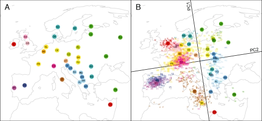
Novembre et al. (2008) compared a two-dimensional PCA map of European samples, obtained by analyzing 197, 146 SNPs in 1,387 individuals from 36 countries, to a geographic map of sampling locations. They examined rotations of the coordinates of the points in the two-dimensional plot of PC1 and PC2, determining the angle of rotation around the origin (PC2,PC1)=(0,0) that maximized the sum of the correlation with longitude of the first coordinate in the rotated PC space and the correlation with latitude of the second coordinate in the rotated PC space. This analysis found that a 16° counterclockwise rotation of the PCA plot most closely resembled the geographic map. To qualitatively demonstrate the resemblance, their Figure 1a provided a striking juxtaposition of the rotated PCA plot alongside a geographic map of Europe. Similar results have been presented by Heath et al. (2008) and Lao et al. (2008).
Figure 1:
Procrustes analysis of genetic and geographic coordinates in Europe, based on data from Novembre et al. (2008). (A) Geographic coordinates for 36 countries. (B) Procrustes-transformed plot of the first two principal components of genetic variation. The plot is centered at the geographic centroid of the populations. Individuals are represented by two- and three-letter abbreviations, and circles represent the centroids of the PCA coordinates for individuals from a country. Abbreviations are as follows: AL, Albania; AT, Austria; BA, Bosnia-Herzegovina; BE, Belgium; BG, Bulgaria; CH, Switzerland; CY, Cyprus; CZ, Czech Republic; DE, Germany; DK, Denmark; ES, Spain; FI, Finland; FR, France; GB, Great Britain; GR, Greece; HR, Croatia; HU, Hungary; IE, Ireland; IT, Italy; KS, Kosovo; LV, Latvia; MK, Macedonia; NL, Netherlands; NO, Norway; PL, Poland; PT, Portugal; RO, Romania; RS, Serbia and Montenegro; RU, Russia; Sct, Scotland; SE, Sweden; SI, Slovenia; SK, Slovakia; TR, Turkey; UA, Ukraine; YG, Yugoslavia. Population labels follow the color scheme of Novembre et al. (2008). The figures are drawn according to the Gall-Peters projection.
With the Procrustes approach, it is further possible to superimpose the Novembre et al. (2008) genetic and geographic maps of Europe in a manner that minimizes the sum across countries of squared distances between geographic coordinates and transformed PCA coordinates. For our analysis, the (PC2,PC1) and (longitude, latitude) coordinates of the samples were kindly shared by J. Novembre. Multiple individuals were sampled per country, with all individuals assumed to have the same geographic coordinates. For each country, from (longitude, latitude) coordinates (λ, φ) measured in degrees, we used the Gall-Peters projection, an equal-area projection that preserves distance along the 45°N parallel, to obtain rectangular coordinates ( ), where R represents the radius of the earth. These geographic coordinates are plotted in Figure 1A.
For each country, we also obtained the centroid on the Novembre et al. (2008) PCA plot of the individuals sampled from the country. Using the 36 pairs of geographic and PCA coordinates, we employed eqs. 2–4 to identify the optimal transformation for aligning the PCA coordinates with the (Gall-Peters-projected) geographic coordinates. This transformation was then applied to the (PC2,PC1) coordinates of all sampled individuals. Figure 1B shows the Procrustes-transformed coordinates of the PCA plot, superimposed on the geographic map of Europe. The centroid of the 36 sets of geographic coordinates and the centroid of the 36 sets of PCA coordinates coincide at 47.539°N 15.498°E, ∼100 km southwest of Vienna, Austria. The rotation applied to the PCA coordinates is 8.860° counterclockwise, reasonably close to the rotation angle of 16° obtained by the method of Novembre et al. (2008). Note, however, that beyond the difference due to our use of Procrustes analysis, two differences exist between our analysis and that of Novembre et al. (2008). First, we applied a projection to the (longitude, latitude) geographic coordinates, whereas Novembre et al. (2008) used unprojected coordinates. When we repeat our Procrustes analysis using unprojected coordinates, we obtain 10.500° for the angle of rotation. Second, in aligning genetic and geographic coordinates, we used centroid coordinates for each country, whereas in the analysis of Novembre et al. (2008), coordinates were aligned at the individual level (treating all individuals from the same country as having identical coordinates). When we repeat our analysis using individual coordinates, we obtain 16.428° for the rotation angle. Further, if we use unprojected geographic coordinates and individual rather than centroid coordinates, as was done by Novembre et al. (2008), we obtain a rotation angle of 16.050°, in close agreement with the 16° angle of Novembre et al. (2008).
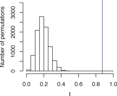
Applying the permutation test with our analysis relying on projected geographic coordinates and population centroids, we find that t0 = 0.874, with P < 0.0001 that a random permutation of the labels in the PCA plot produces greater similarity to the geographic coordinates than that seen with the correct labels (Figure 2). Thus, the pattern of relative distances among points in the PCA plot has a demonstrably high degree of similarity to the corresponding pattern of relative distances in the geographic map. Through a quantitative assessment of this similarity, our computations confirm the qualitatively striking concordance of genetics and geography reported by Novembre et al. (2008).
Figure 2:
Distribution of the permutation test statistic t, comparing a geographic map of sampling locations (Figure 1A) and a SNP-based PCA map (Figure 1B) in European populations. The value of t0, the permutation test statistic obtained from the unpermuted data, is represented by the blue vertical line, and it equals 0.874 (P < 0.0001).
Genes and geography worldwide
We next performed an analogous alignment of coordinates computed from genetic data to geographic sampling locations, for samples collected worldwide. In an analysis of 512,762 SNPs in 443 individuals from 29 worldwide human populations, Jakobsson et al. (2008) obtained a two-dimensional MDS plot on the basis of an individual-level pairwise allele-sharing genetic distance matrix. Qualitatively, the MDS plot resembled a geographic map of the sampling locations, with the axes corresponding largely to latitude and longitude. This same phenomenon is visible in the work of Li et al. (2008) and Biswas et al. (2009).
To quantitatively assess the resemblance, we Procrustes-transformed SNP-based MDS coordinates to produce an optimal alignment with geographic coordinates. For this analysis, we used coordinates of an MDS plot based on a population-level genetic distance matrix. We used microsat (Minch et al., 1998) to obtain the allele-sharing genetic distance matrix (Mountain and Cavalli-Sforza, 1997) between populations for the data of Jakobsson et al. (2008). Classical metric multidimensional scaling was applied to the matrix, using the cmdscale command in R (Ihaka and Gentleman, 1996). For the geographic coordinates, we used (Gall-Peters-projected) latitudes and longitudes from Table S6 of Jakobsson et al. (2008).
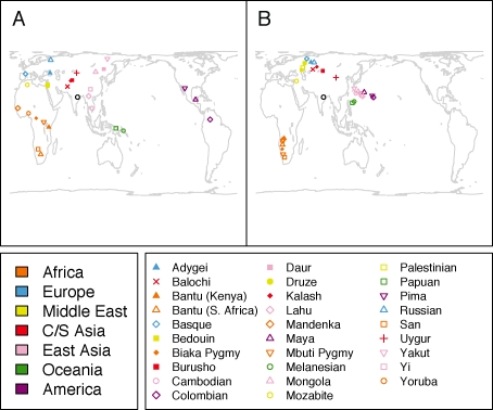
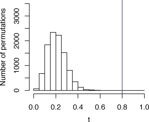
Figure 3A shows the geographic coordinates of the 29 populations, drawn on a world map. Figure 3B provides the Procrustes-transformed two-dimensional MDS plot of the genetic data. Although genetic coordinates for some populations are quite distant from the corresponding sampling locations, a geographic pattern in the MDS plot is clear. The value of t0 for the genetic and geographic coordinates is 0.799 (P < 0.0001), considerably exceeding the similarity values for all 10,000 permutations examined for the labels in the MDS plot (Figure 4). As was true in the case of Europeans, a formal quantitative comparison supports the qualitative resemblance of genetic coordinates to geographic coordinates.
Figure 3:
Procrustes analysis of genetic and geographic coordinates worldwide, based on data from Jakobsson et al. (2008). (A) Geographic coordinates for 29 populations. (B) Procrustes-transformed MDS plot of genetic variation. The figures are drawn according to the Gall-Peters projection. For each graph, the black open circle represents the centroid of the points plotted.
Figure 4:
Distribution of the permutation test statistic t, comparing a geographic map of sampling locations (Figure 3A) and a SNP-based MDS map (Figure 3B) in worldwide populations. The value of t0, the permutation test statistic obtained from the unpermuted data, is represented by the blue vertical line, and it equals 0.799 (P < 0.0001).
MDS and PCA
Our next example considered the similarity of MDS and PCA plots obtained on the basis of SNP data in overlapping worldwide samples. In particular, we compared the individual-level two-dimensional MDS plot of Jakobsson et al. (2008) with the corresponding individual-level PCA plot of the first two principal components in Biswas et al. (2009). For the MDS plot, we used coordinates from the individual-level SNP-based MDS plot presented by Jakobsson et al. (2008), in which MDS was performed on an individual-level allele-sharing genetic distance matrix. The PCA coordinates from Biswas et al. (2009) were based on the analysis of 643,884 autosomal SNPs and 944 unrelated individuals from 52 populations (Li et al., 2008), using SNP genotypes normalized according to eq. 3 of Patterson et al. (2006). PCA coordinates from Biswas et al. (2009) were kindly shared by J. Akey. The datasets underlying the MDS and PCA plots have considerable overlap, in that 433 individuals are included in both datasets.
We applied Procrustes analysis to the common set of 433 individuals, represented by 433 pairs of points, one each in the MDS and PCA plots. The 433 points in the PCA plot were transformed to produce an optimal alignment with the 433 corresponding points in the MDS plot. The optimal transformation was then applied to all 944 points in the PCA plot.
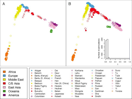
Figure 5A shows the individual-level MDS plot of genetic data, in which 443 individuals from 29 populations are included (Jakobsson et al., 2008). The orientation of this figure was determined by Procrustes transformation, aligning individual-level MDS coordinates to the geographic coordinates of the individuals. Figure 5B shows the Procrustes-transformed PCA plot with all 944 individuals from 52 populations included. The two plots are quite similar, with the larger number of points present in the PCA plot filling in gaps visible in the MDS plot. Considering 10,000 permutations of the labels in the PCA plot of the 433 shared points, we find that t0 = 0.993 with P < 0.0001. This high value of t0 indicates a very strong concordance between MDS and PCA in analyzing the data, as is expected given the close relationship of these two techniques (indeed, for a given use of PCA, a certain special case of MDS produces identical results (Mardia et al., 1979)). The example further illustrates how Procrustes analysis can be used to compare two plots in which the sets of points only partially overlap.
Figure 5:
Procrustes analysis of genetic coordinates obtained using MDS and PCA. (A) MDS plot of genetic variation for 443 individuals from 29 worldwide populations, based on data from Jakobsson et al. (2008). (B) Procrustes-transformed PCA plot of genetic variation for 944 individuals from 52 worldwide populations, based on data from Biswas et al. (2009). The Procrustes analysis relies on a subset of 433 individuals included in both datasets. Note that unlike Biswas et al., our plot splits the Han and Han (N. China) groups, so that the 944 individuals are separated into 53 populations rather than 52. A histogram of the t statistic across 10,000 permutations appears in the lower right corner (t0 = 0.993, P < 0.0001).
SNPs and CNVs
Our final comparison examined the similarity of MDS plots obtained using different types of markers collected in the same samples. We compared an MDS plot on the basis of 396 copy-number-variable loci reported by Jakobsson et al. (2008) to the SNP-based MDS plot in the same worldwide populations. The population-level CNV genetic distance matrix was obtained as in Jakobsson et al. (2008). MDS and Procrustes computations were conducted in the same manner as in the analysis of worldwide SNPs and geography.
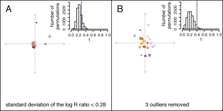
The CNV-based and SNP-based MDS plots are qualitatively dissimilar, with the SNP-based plot (Figure 3B) resembling the geographic sampling locations (Figure 3A), and the CNV-based plot (Figure 6A) instead having all except three points located near the center. The similarity statistic between the CNV-based and SNP-based plots reflects this relative discordance (t0 = 0.285, P = 0.1536). Removal from the two MDS plots of the three outlier populations — Kalash, Melanesian, and Papuan — followed by reapplication of Procrustes analysis leads to greater qualitative similarity (Figure 6B). Although the similarity statistics in Figures 6A and 6B are not strictly comparable because of the different numbers of points in the two plots, it is noteworthy that upon removal of the outliers, the t statistic between the CNV-based and SNP-based MDS plots increases to t0 = 0.400 (P = 0.0292).
Figure 6:
Procrustes analysis of CNV-based MDS genetic coordinates. (A) Procrustes-transformed MDS plot for CNV data, aligned to the SNP-based MDS plot in Figure 3B. A histogram of the t statistic across 10,000 permutations appears in the upper right corner (t0 = 0.285, P = 0.1536). A version of the MDS plot without the Procrustes transformation appeared in Figure S14 of Jakobsson et al. (2008). (B) Procrustes-transformed CNV-based MDS plot, excluding three outliers, aligned to the restriction of the SNP-based MDS plot in Figure 3B to the 26 non-outlier populations. The three outlier populations are Kalash, Melanesian, and Papuan. A histogram of the t statistic across 10,000 permutations appears in the upper right corner (t0 = 0.400, P = 0.0292). The population labels and colors follow those of Figure 3, and for each graph, the center of the cross represents the centroid of the points plotted.
The importance of the three outlier populations in determining the nature of the axes in the CNV-based MDS plot is potentially a consequence of high genetic distances in comparisons involving these populations (Table S1 of Jakobsson et al. (2008)). These high distances result from high numbers of CNVs detected in the three outlier populations (Jakobsson et al., 2008), which in turn might trace to high values in these populations of a tuning parameter used in the CNV genotyping assays (Itsara et al., 2009). CNV genotypes were obtained using PennCNV (Wang et al., 2007) applied to genome-wide genotyping intensity signals. For a given sample, the variability of genotyping intensity across the genome influences the ability of PennCNV to identify CNVs (Wang et al., 2007; Itsara et al., 2009). The “standard deviation of the log R ratio,” henceforth denoted s, provides a measure of this variability, where the log R ratio at a given (biallelic) site considers log2 of the ratio of the genotyping intensity for one allelic type to the intensity for the other type. Higher values of s lead to greater difficulty in accurate CNV identification by PennCNV, systematically giving rise to additional false-positive CNV detections.
The Procrustes approach enables us to assess the hypothesis that the dissimilarity of the CNV-based and SNP-based MDS plots in Figures 6A and 3B ultimately traces to high-s low-quality genotyping assays in outlier populations. We first varied the maximal value of s allowed for samples included in the analysis. Among 443 unrelated individuals studied by Jakobsson et al. (2008), the CNV-based MDS plot in Figure 6A utilized 405 of these individuals, each with s < 0.28. Starting from this set of 405 individuals, we generated nine datasets based on nine values of the upper bound on s for samples included in the analysis. These choices for the cutoff on s were selected at intervals of 0.01 from 0.20 to 0.28. The choice of 0.28, used by Jakobsson et al. (2008), matches that of Figure 6 and is the most permissive, producing a dataset with the most CNVs, but with potentially more false-positive CNV identifications. The choice of 0.20 is the most restrictive, leading to a smaller dataset with fewer samples, but also with fewer false positives. For each cutoff choice, samples were excluded from the initial collection of 405 individuals if their s values were greater than or equal to the cutoff (exclusions of s values strictly greater than the cutoff would have produced the same datasets). Using each reduced set of individuals, CNV loci that were polymorphic in the set were identified, and non-singleton autosomal CNVs were retained for MDS analysis. In some populations, as few as two individuals were retained in reduced datasets (Table 1), but each of the nine datasets included individuals from all populations (Table 2). To ensure that all datasets included at least two individuals from each population, we did not consider cutoff choices below 0.20.
Table 1:
Sizes of CNV datasets reduced according to cutoffs on the standard deviation of the log R ratio.
| Cutoff on the standard deviation of the log R ratio (s) | Number of individuals including relatives | Number of individuals excluding relatives | Smallest sample size across populations when excluding relatives | Number of autosomal non-singleton CNV loci when excluding relatives |
|---|---|---|---|---|
| 0.20 | 351 | 320 | 2 | 208 |
| 0.21 | 371 | 340 | 3 | 231 |
| 0.22 | 386 | 355 | 3 | 243 |
| 0.23 | 402 | 370 | 4 | 255 |
| 0.24 | 413 | 379 | 4 | 272 |
| 0.25 | 418 | 384 | 5 | 285 |
| 0.26 | 425 | 389 | 5 | 298 |
| 0.27 | 431 | 395 | 5 | 332 |
| 0.28 | 443 | 405 | 5 | 396 |
Table 2:
Number of unrelated individuals in each of 29 populations, in CNV datasets reduced according to cutoffs on the standard deviation of the log R ratio.
| Number of unrelated individuals in reduced CNV datasets | |||||||||
|---|---|---|---|---|---|---|---|---|---|
| Population | s < 0.20 | s < 0.21 | s < 0.22 | s < 0.23 | s < 0.24 | s < 0.25 | s < 0.26 | s < 0.27 | s < 0.28 |
| Adygei | 9 | 10 | 10 | 12 | 12 | 12 | 12 | 13 | 13 |
| Balochi | 11 | 12 | 13 | 14 | 14 | 14 | 14 | 14 | 14 |
| Bantu (Kenya) | 10 | 10 | 10 | 10 | 10 | 10 | 10 | 11 | 11 |
| Bantu (S. Africa) | 7 | 7 | 7 | 7 | 7 | 7 | 7 | 7 | 7 |
| Basque | 6 | 7 | 11 | 11 | 11 | 11 | 11 | 11 | 11 |
| Bedouin | 37 | 40 | 40 | 40 | 40 | 40 | 41 | 41 | 41 |
| Biaka Pygmy | 19 | 19 | 19 | 21 | 22 | 22 | 22 | 22 | 23 |
| Burusho | 5 | 5 | 5 | 6 | 6 | 6 | 6 | 6 | 6 |
| Cambodian | 10 | 10 | 10 | 10 | 10 | 10 | 10 | 10 | 10 |
| Colombian | 7 | 7 | 7 | 7 | 7 | 7 | 7 | 7 | 7 |
| Daur | 8 | 8 | 8 | 8 | 9 | 9 | 9 | 10 | 10 |
| Druze | 31 | 32 | 33 | 33 | 33 | 34 | 34 | 34 | 35 |
| Kalash | 2 | 5 | 5 | 6 | 6 | 6 | 6 | 7 | 12 |
| Lahu | 8 | 8 | 8 | 8 | 8 | 8 | 8 | 8 | 8 |
| Mandenka | 20 | 20 | 20 | 20 | 21 | 22 | 22 | 22 | 22 |
| Maya | 3 | 4 | 4 | 4 | 4 | 7 | 8 | 8 | 8 |
| Mbuti Pygmy | 9 | 10 | 11 | 11 | 12 | 12 | 12 | 12 | 12 |
| Melanesian | 5 | 5 | 6 | 6 | 6 | 6 | 6 | 6 | 7 |
| Mongola | 6 | 7 | 7 | 9 | 9 | 9 | 9 | 9 | 9 |
| Mozabite | 26 | 28 | 28 | 28 | 28 | 28 | 28 | 28 | 28 |
| Palestinian | 19 | 20 | 21 | 22 | 23 | 23 | 23 | 23 | 23 |
| Papuan | 7 | 7 | 7 | 8 | 8 | 8 | 8 | 10 | 12 |
| Pima | 2 | 3 | 3 | 4 | 5 | 5 | 5 | 5 | 5 |
| Russian | 3 | 5 | 7 | 9 | 12 | 12 | 13 | 13 | 13 |
| San | 5 | 5 | 6 | 6 | 6 | 6 | 6 | 6 | 6 |
| Uygur | 9 | 9 | 9 | 9 | 9 | 9 | 9 | 9 | 9 |
| Yakut | 6 | 7 | 9 | 10 | 10 | 10 | 12 | 12 | 12 |
| Yi | 8 | 8 | 9 | 9 | 9 | 9 | 9 | 9 | 9 |
| Yoruba | 22 | 22 | 22 | 22 | 22 | 22 | 22 | 22 | 22 |
MDS analyses of the eight new CNV datasets proceeded using the same methods as were used in the analysis of the initial s < 0.28 dataset. For each CNV dataset, we constructed an allele-sharing population-level genetic distance matrix in the same manner as was done by Jakobsson et al. (2008) for the s < 0.28 dataset. We then performed MDS and used Procrustes analysis to compare the resulting plots to the SNP-based MDS plot in Figure 3B.
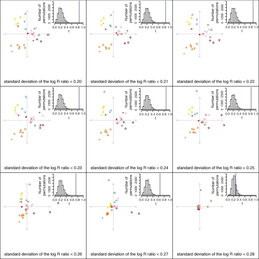
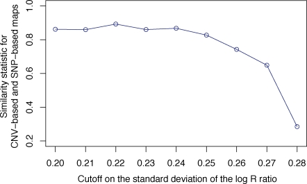
Figure 7 displays the Procrustes-transformed CNV-based MDS plots based on the nine choices of the cutoff on s. As the cutoff decreases, the resemblance of the MDS plot to the SNP-based MDS plot in Figure 3B increases. The smallest values of the cutoff on s lead to MDS plots with a similar triangular structure to the plot obtained with SNPs: populations from Africa lie in the lower left corner, populations from the Middle East and Europe lie near the top, populations from the Americas lie on the right, and populations from Asia lie along an upper edge. The values of t0 are greatest for the lowest values of the cutoff, and all plots except the s < 0.28 plot produce P < 0.0001. Figure 8 shows that for cutoffs of 0.25 or less, t0 is quite high, greater even than the value of t0 for the comparison of SNPs and geography in Figure 4. The t0 statistic is somewhat lower with cutoffs s < 0.26 and s < 0.27, and it is considerably lower with the original cutoff of s < 0.28.
Figure 7:
Procrustes analysis of CNV-based MDS genetic coordinates, for nine separate choices of the cutoff on s for inclusion of samples in the CNV data. Each graph represents a Procrustes-transformed MDS plot for the CNV data based on a particular choice of the cutoff on s, aligned to the SNP-based MDS plot in Figure 3B. The s < 0.28 MDS plot is the same as the plot in Figure 6A. In increasing order of the cutoff on s, the values of t0 are 0.862, 0.859, 0.892, 0.860, 0.867, 0.827, 0.742, 0.648, and 0.285. For the cutoff of 0.28, P = 0.1536, and for all other cutoffs, P < 0.0001. The population labels and colors follow those of Figure 3, and for each graph, the center of the cross represents the centroid of the points plotted.
Figure 8:
Relationship of the t0 similarity statistic between CNV-based and SNP-based MDS plots to the cutoff on the standard deviation of the log R ratio.
Thus, Procrustes analysis of reduced CNV datasets suggests that CNVs produce similar patterns of population structure to those observed with SNPs. When restricting the CNV dataset to smaller sets of individuals with more reliable CNV detection, as represented by lower values of s, the similarity of CNV-based MDS plots to the SNP-based MDS plot increases. This result supports the view that high values of s for certain individuals from the Kalash, Melanesian, and Papuan populations explain the outlier status of these populations in previous analysis of CNV population structure (Jakobsson et al., 2008). As suggested by Itsara et al. (2009), it is likely that high-s individuals produce numerous false-positive CNV genotypes; however, removal of these individuals only reinforces the observation of Jakobsson et al. (2008) that a general similarity exists between CNV-based and SNP-based inferences of population structure.
Discussion
The Procrustes approach for investigating the concordance of separate sets of spatial positions has been used for diverse biological problems, particularly in the context of morphometric data (Bookstein, 1996; Dryden and Mardia, 1998; Adams et al., 2004). We suggest that this approach similarly has considerable potential for use with population-genetic data. Our examples quantitatively comparing genes and geography through the use of Procrustes analysis strengthen the evidence for patterns previously identified qualitatively. They support a strong role for geography in predicting patterns of population structure, both in Europe and worldwide. Our Procrustes example with CNV-based and SNP-based MDS plots shows that the similarity of CNV-based inference of human population structure to SNP-based inference is greater than had been reported previously with a permissive cutoff for sample inclusion in CNV analysis.
In agreement with Itsara et al. (2009), our Procrustes analysis supports the view that the difference between CNV-based and SNP-based inference in our previous work (Jakobsson et al., 2008) was due to use of a permissive cutoff. However, in contrast to the claim of Itsara et al. (2009) that there is “limited evidence for stratification of CNVs in geographically distinct human populations,” our use of a more restrictive cutoff leads to the conclusion that population structure is detectable on the basis of CNVs, and that the CNV population structure pattern has a strong concordance with that inferred using SNPs. The concordance between CNV-based and SNP-based MDS plots, t0 = 0.892 for the s < 0.22 cutoff on the standard deviation of the log R ratio, exceeds the concordance between the SNP-based MDS plot and the geographic coordinates of sampling locations.
We note that many alternatives to the Procrustes approach exist for aligning sets of points, including methods that are robust to the presence of outliers (Rohlf and Slice, 1990; Dryden and Mardia, 1998). In addition, the Mantel coefficient (Mantel, 1967; Sokal and Rohlf, 1995) and the RV coefficient (Robert and Escoufier, 1976; Heo and Gabriel, 1998) provide alternatives to the Procrustes t statistic for measuring the similarity of pairs of plots. To compare t and the RV coefficient, for each of the CNV-based MDS plots in Figure 7, we repeated our comparisons to the SNP-based MDS plot in Figure 3B, substituting the RV coefficient in place of the t statistic. The correlation of RV and t across the nine plots was high (r = 0.994), and P-values from permutation tests with RV were similar to those with t (P = 0.2836 for the s < 0.28 plot and P < 0.0001 for all other plots). However, while the t statistic and the RV coefficient appear to perform similarly, t is perhaps more intuitive in the Procrustes context, as it is a simple function of the sum of squared Euclidean distances between corresponding points in the two plots when the plots are optimally aligned.
The computations we have performed involve comparisons of genes and geography, comparisons of results from two separate multivariate analysis techniques (PCA and MDS), and comparisons of inferences from separate types of markers. However, the Procrustes approach has several other potential uses in population genetics. The Procrustes t statistic can provide a method for comparing PCA or MDS plots based on observed data to those based on simulations, thereby assisting in evaluating the fit of PCA and MDS patterns in population-genetic data to those that population-genetic models predict. The Procrustes approach also enables the comparison of variant analyses performed with the same multivariate analysis technique, such as in examining MDS plots based on different genetic distances or based on different bootstrap replicates. As in our example comparing PCA results of Biswas et al. (2009) and MDS results of Jakobsson et al. (2008), Procrustes analysis can be used in integrating separate results on the basis of sample sets that overlap only partially. In our investigation of multiple analyses of CNVs, we based the comparison on similarity to a reference dataset; if no natural basis exists for selecting a particular dataset as the reference, such as in comparing multiple genetic distances, bootstrap replicates, or repeated simulations, a generalized Procrustes technique can be used, in which results from the various analyses are transformed iteratively until a sum considering all pairs of configurations cannot be further reduced (Gower, 1975; Dryden and Mardia, 1998). In all these applications, Procrustes methods can make the results of separate analyses of standard data sets commensurable. Further, Procrustes analysis is applicable to data both in two dimensions and in higher-dimensional spaces for which no simple visual alternative exists. Thus, the examples we have considered represent only a small subset of the category of problems in population genetics for which the Procrustes approach might provide an informative tool for data analysis.
Footnotes
We are grateful to J. Akey and J. Novembre for assistance with the data from their papers. We thank T. Jombart and an anonymous reviewer for comments on the manuscript. This work was supported in part by NIH grants R01 GM081441 and T32 GM070449, by a Burroughs Wellcome Fund Career Award in the Biomedical Sciences, by an Alfred P. Sloan Research Fellowship, and by the Intramural Research Program of the National Institute on Aging, National Institutes of Health, Department of Health and Human Services (project number Z01-AG000932-02).
References
- Adams DC, Rohlf FJ, Slice DE. Geometric morphometrics: ten years of progress following the ‘revolution’. Ital J Zool. 2004;71:5–16. doi: 10.1080/11250000409356545. [DOI] [Google Scholar]
- Biswas S, Scheinfeldt LB, Akey JM. Genome-wide insights into the patterns and determinants of fine-scale population structure in humans. Am J Hum Genet. 2009;84:641–650. doi: 10.1016/j.ajhg.2009.04.015. [DOI] [PMC free article] [PubMed] [Google Scholar]
- Bookstein FL. Biometrics, biomathematics and the morphometric synthesis. Bull Math Biol. 1996;58:313–365. doi: 10.1007/BF02458311. [DOI] [PubMed] [Google Scholar]
- Chen J, Zheng H, Bei JX, Sun L, Jia WH, Li T, Zhang F, Seielstad M, Zeng YX, Zhang X, Liu J. Genetic structure of the Han Chinese population revealed by genome-wide SNP variation. Am J Hum Genet. 2009;85:775–785. doi: 10.1016/j.ajhg.2009.10.016. [DOI] [PMC free article] [PubMed] [Google Scholar]
- Cox TF, Cox MAA. Multidimensional Scaling. 2nd ed. Boca Raton: Chapman & Hall; 2001. [Google Scholar]
- Dryden IL, Mardia KV. Statistical Shape Analysis. Chichester: Wiley; 1998. [Google Scholar]
- Gower JC. Generalized Procrustes analysis. Psychometrika. 1975;40:33–51. doi: 10.1007/BF02291478. [DOI] [Google Scholar]
- Gower JC, Dijksterhuis GB. Procrustes Problems. Oxford University Press; 2004. [Google Scholar]
- Heath SC, Gut IG, Brennan P, McKay JD, Bencko V, Fabianova E, Foretova L, Georges M, Janout V, Kabesch M, Krokan HE, Elvestad MB, Lissowska J, Mates D, Rudnai P, Skorpen F, Schreiber S, Soria JM, Syvänen AC, Meneton P, Herçberg S, Galan P, Szeszenia-Dabrowska N, Zaridze D, Génin E, Cardon LR, Lathrop M. Investigation of the fine structure of European populations with applications to disease association studies. Eur J Hum Genet. 2008;16:1413–1429. doi: 10.1038/ejhg.2008.210. [DOI] [PubMed] [Google Scholar]
- Heo M, Gabriel KR. A permutation test of association between configurations by means of the RV coefficient. Commun Stat Simul Comp. 1998;27:843–856. doi: 10.1080/03610919808813512. [DOI] [Google Scholar]
- Ihaka R, Gentleman R. R: a language for data analysis and graphics. J Comput Graph Stat. 1996;5:299–314. doi: 10.2307/1390807. [DOI] [Google Scholar]
- Itsara A, Cooper GM, Baker C, Girirajan S, Li J, Absher D, Krauss RM, Myers RM, Ridker PM, Chasman DI, Mefford H, Ying P, Nickerson DA, Eichler EE. Population analysis of large copy number variants and hotspots of human genetic disease. Am J Hum Genet. 2009;84:148–161. doi: 10.1016/j.ajhg.2008.12.014. [DOI] [PMC free article] [PubMed] [Google Scholar]
- Jackson DA. PROTEST: a Procrustean randomization test of community environment. Ecoscience. 1995;2:297–303. [Google Scholar]
- Jakkula E, Rehnström K, Varilo T, Pietiläinen OPH, Paunio T, Pedersen NL, deFaire U, Järvelin MR, Saharinen J, Freimer N, Ripatti S, Purcell S, Collins A, Daly MJ, Palotie A, Peltonen L. The genome-wide patterns of variation expose significant substructure in a founder population. Am J Hum Genet. 2008;83:787–794. doi: 10.1016/j.ajhg.2008.11.005. [DOI] [PMC free article] [PubMed] [Google Scholar]
- Jakobsson M, Scholz SW, Scheet P, Gibbs JR, VanLiere JM, Fung HC, Szpiech ZA, Degnan JH, Wang K, Guerreiro R, Bras JM, Schymick JC, Hernandez DG, Traynor BJ, Simon-Sanchez J, Matarin M, Britton A, van de Leemput J, Rafferty I, Bucan M, Cann HM, Hardy JA, Rosenberg NA, Singleton AB. Genotype, haplotype, and copy-number variation in worldwide human populations. Nature. 2008;451:998–1003. doi: 10.1038/nature06742. [DOI] [PubMed] [Google Scholar]
- Jombart T, Pontier D, Dufour AB. Genetic markers in the playground of multivariate analysis. Heredity. 2009;102:330–341. doi: 10.1038/hdy.2008.130. [DOI] [PubMed] [Google Scholar]
- Lao O, Lu TT, Nothnagel M, Junge O, Freitag-Wolf S, Caliebe A, Balascakova M, Bertranpetit J, Bindoff LA, Comas D, Holmlund G, Kouvatsi A, Macek M, Mollet I, Parson W, Palo J, Ploski R, Sajantila A, Tagliabracci A, Gether U, Werge T, Rivadeneira F, Hofman A, Uitterlinden AG, Gieger C, Wichmann HE, Rüther A, Schreiber S, Becker C, Nürnberg P, Nelson MR, Krawczak M, Kayser M. Correlation between genetic and geographic structure in Europe. Curr Biol. 2008;18:1241–1248. doi: 10.1016/j.cub.2008.07.049. [DOI] [PubMed] [Google Scholar]
- Li JZ, Absher DM, Tang H, Southwick AM, Casto AM, Ramachandran S, Cann HM, Barsh GS, Feldman M, Cavalli-Sforza LL, Myers RM. Worldwide human relationships inferred from genome-wide patterns of variation. Science. 2008;319:1100–1104. doi: 10.1126/science.1153717. [DOI] [PubMed] [Google Scholar]
- Mantel N. The detection of disease clustering and a generalized regression approach. Cancer Res. 1967;27:209–220. [PubMed] [Google Scholar]
- Mardia KV, Kent JT, Bibby JM. Multivariate Analysis. London: Academic Press; 1979. [Google Scholar]
- McVean G. A genealogical interpretation of principal components analysis. PLoS Genet. 2009;5:e1000686. doi: 10.1371/journal.pgen.1000686. [DOI] [PMC free article] [PubMed] [Google Scholar]
- Menozzi P, Piazza A, Cavalli-Sforza L. Synthetic maps of human gene frequencies in Europeans. Science. 1978;201:786–792. doi: 10.1126/science.356262. [DOI] [PubMed] [Google Scholar]
- Minch E, Ruiz Linares A, Goldstein DB, Feldman MW, Cavalli-Sforza LL. MICROSAT (version 2alpha): a program for calculating statistics on microsatellite data. Department of Genetics, Stanford University; Stanford, CA: 1998. [Google Scholar]
- Mountain JL, Cavalli-Sforza LL. Multilocus genotypes, a tree of individuals, and human evolutionary history. Am J Hum Genet. 1997;61:705–718. doi: 10.1086/515510. [DOI] [PMC free article] [PubMed] [Google Scholar]
- Novembre J, Johnson T, Bryc K, Kutalik Z, Boyko AR, Auton A, Indap A, King KS, Bergmann S, Nelson MR, Stephens M, Bustamante CD. Genes mirror geography within Europe. Nature. 2008;456:98–101. doi: 10.1038/nature07331. [DOI] [PMC free article] [PubMed] [Google Scholar]
- Novembre J, Stephens M. Interpreting principal component analyses of spatial population genetic variation. Nature Genet. 2008;40:646–649. doi: 10.1038/ng.139. [DOI] [PMC free article] [PubMed] [Google Scholar]
- Patterson N, Price AL, Reich D. Population structure and eigenanalysis. PLoS Genet. 2006;2:2074–2093. doi: 10.1371/journal.pgen.0020190. [DOI] [PMC free article] [PubMed] [Google Scholar]
- Peres-Neto PR, Jackson DA. How well do multivariate data sets match? The advantages of a Procrustean superimposition approach over the Mantel test. Oecologia. 2001;129:169–178. doi: 10.1007/s004420100720. [DOI] [PubMed] [Google Scholar]
- Price AL, Helgason A, Palsson S, Stefansson H, St. Clair D, Andreassen OA, Reich D, Kong A, Stefansson K. The impact of divergence time on the nature of population structure: an example from Iceland. PLoS Genet. 2009;5:e1000505. doi: 10.1371/journal.pgen.1000505. [DOI] [PMC free article] [PubMed] [Google Scholar]
- Ramachandran S, Deshpande O, Roseman CC, Rosenberg NA, Feldman MW, Cavalli-Sforza LL. Support from the relationship of genetic and geographic distance in human populations for a serial founder effect originating in Africa. Proc. Natl. Acad. Sci USA. 2005;102:15942–15947. doi: 10.1073/pnas.0507611102. [DOI] [PMC free article] [PubMed] [Google Scholar]
- Robert P, Escoufier Y. A unifying tool for linear multivariate statistical methods: the RV-coefficient. J. Roy. Statist. Soc. Ser C. 1976;25:257–265. [Google Scholar]
- Rohlf FJ, Slice D. Extensions of the Procrustes method for the optimal superimposition of landmarks. Syst Zool. 1990;39:40–59. doi: 10.2307/2992207. [DOI] [Google Scholar]
- Sokal RR, Rohlf FJ. Biometry. 3rd ed. New York: Freeman; 1995. [Google Scholar]
- Tian C, Kosoy R, Lee A, Ransom M, Belmont JW, Gregersen PK, Seldin MF. Analysis of East Asia genetic substructure using genome-wide SNP arrays. PLoS One. 2008;3:e3862. doi: 10.1371/journal.pone.0003862. [DOI] [PMC free article] [PubMed] [Google Scholar]
- Wang K, Li M, Hadley D, Liu R, Glessner J, Grant SFA, Hakonarson H, Bucan M. PennCNV: an integrated hidden Markov model designed for high-resolution copy number variation detection in whole-genome SNP genotyping data. Genome Res. 2007;17:1665–1674. doi: 10.1101/gr.6861907. [DOI] [PMC free article] [PubMed] [Google Scholar]
- Xu S, Yin X, Li S, Jin W, Lou H, Yang L, Gong X, Wang H, Shen Y, Pan X, He Y, Yang Y, Wang Y, Fu W, An Y, Wang J, Tan J, Qian J, Chen X, Zhang X, Sun Y, Zhang X, Wu B, Jin L. Genomic dissection of population substructure of Han Chinese and its implication in association studies. Am J Hum Genet. 2009;85:762–774. doi: 10.1016/j.ajhg.2009.10.015. [DOI] [PMC free article] [PubMed] [Google Scholar]
- Zhivotovsky LA, Rosenberg NA, Feldman MW. Features of evolution and expansion of modern humans, inferred from genomewide microsatellite markers. Am J Hum Genet. 2003;72:1171–1186. doi: 10.1086/375120. [DOI] [PMC free article] [PubMed] [Google Scholar]


