Binocular combination in anisometropic amblyopia

Abstract

Using a suprathreshold binocular summation paradigm developed by J. Ding and G. Sperling (2006, 2007) for normal observers, we investigated suprathreshold cyclopean perception in anisometropic amblyopia. In this paradigm, two suprathreshold sinewave gratings of the same spatial frequency but different spatial phases are presented to the left and right eyes of the observer. The perceived phase of the binocularly combined cyclopean image is measured as a function of the contrast ratio between the images in the two eyes. We found that both eyes contributed equally in normal subjects. However, stimulus of equal contrast was weighted much less in the amblyopic eye relative to the fellow eye in binocular combination. For the five amblyopes, the effective contrast of the amblyopic eye in binocular combination is equal to about 11%–28% of the same contrast presented to the fellow eye, much less than the ratio of contrast sensitivity between the two eyes (0.73–1.42). The results from the current study have many important implications in amblyopia research and treatment.

Introduction

Binocular vision is extremely important in human visual perception (Howard & Rogers, 1995). In addition to its critical role in depth perception, binocular vision improves human performance in many complex visual tasks that do not involve depth perception, such as reading, detecting camouflaged objects, and eye-hand coordination (Jones & Lee, 1981; Sheedy, Bailey, Buri, & Bass, 1986). Normal binocular vision requires two normal monocular visual systems as well as their normal interactions. Various monocular and binocular abnormalities of the visual system have been shown to lead to deficient binocular vision (Donzis, Rappazzo, Burde, & Gordon, 1983; Goodwin & Romano, 1985; Halpern & Blake, 1988; Legge & Gu, 1989). In this study, we investigated the nature of binocular visual deficits in anisometropic amblyopia.

Amblyopia is a clinical condition that affects about 3% of the population (Ciuffreda, Levi, & Selenow, 1991). It is characterized by reduced visual acuity that is not associated with any detectable organic defects and cannot be corrected by refractive means. Although often regarded as a result of early abnormal visual experience, such as uncorrected strabismus, anisometropia, or form deprivation caused by cataract, the mechanisms underlying amblyopia are still under investigation (Daw, 1998; Kiorpes, Tang, & Movshon, 1999).

In addition to decreased letter acuity, numerous studies have found that amblyopia may affect a variety of spatial vision functions, ranging from contrast sensitivity (Bradley & Freeman, 1981; Hess & Howell, 1977; Levi & Harwerth, 1978), stereoacuity (Walraven & Janzen, 1993), hyperacuity (Kelly & Buckingham, 1998; Levi & Klein, 1982), phase sensitivity (Lawden, Hess, & Campbell, 1982; Pass & Levi, 1982) and motion perception (Simmers, Ledgeway, Hess, & McGraw, 2003) to shape perception (Levi, Li, & Klein, 2005), contour integration (Hess, McIlhagga, & Field, 1997), spatial lateral interaction (Bonneh, Sagi, & Polat, 2004, 2007; Levi, Hariharan, & Klein, 2002) and visual counting (Sharma, Levi, & Klein, 2000).

Although most research in amblyopia has focused on monocular deficits in the amblyopic eye, studies have also documented abnormal binocular vision in amblyopia. For example, Goodwin and Romano (1985) found that reduction of stereoacuity was highly correlated with reduction of both monocular and binocular visual acuity in anisometropic amblyopia. Holopigian, Blake, and Greenwald (1986) found that, for anisometropic amblyopes, stereoacuity is normal at low spatial frequencies, subnormal at intermediate spatial frequencies, and very poor at higher spatial frequencies, and, for strabismic amblyopes, stereoacuity is abnormal at all spatial frequencies. On the other hand, binocular motion integration is largely normal in anisometropic amblyopia (McKee, Levi, & Movshon, 2003). Recently, Baker, Meese, Mansouri, and Hess (2007) also found that binocular summation is normal in strabismic amblyopes after the contrasts of the two monocular inputs are normalized by the contrast sensitivities of the corresponding eyes (Baker et al., 2007). They attributed earlier observations of lack of binocular summation in amblyopia (Holopigian et al., 1986; Hood & Morrison, 2002; Lema & Blake, 1977; Levi, Harwerth, & Manny, 1979; Levi, Harwerth, & Smith, 1980; McKee et al., 2003; Pardhan & Gilchrist, 1992) to the experimental procedures that did not compensate for different sensitivities between the amblyopic and fellow eyes.

Many studies have also documented abnormal interocular interactions in amblyopia. Studies found that stimulation of the fellow eye increased the luminance threshold (Flynn, McKenney, & Dannheim, 1971), reduced the visual acuity (Pugh, 1954), and increased the size and depth of the suppression scotoma in the amblyopic eye (Pratt-Johnson, 1969). Mitchell, Reardon, and Muir (1975) found no interocular transfer of motion after-effects at all in one anisometropic, one strabismic, and one strabismic/anisometropic amblyopes. Stimulating both the amblyopic and fellow eyes of anisometropic amblyopes, Wood, Fox, and Stephenson (1978) found that contrast thresholds of random dot stereograms were elevated in both eyes. Several human studies (Agrawal, Conner, Odom, Schwartz, & Mendola, 2006; McKee et al., 2003) and animal (Kiorpes & McKee, 1999) concluded that the severity of binocularity loss might sometimes better predict the nature of physiological changes in amblyopia than clinical etiology. In other words, the degree of binocularity may at least partially predict abnormality in monocular tasks.

A number of dichoptic contrast masking experiments concluded that there is much stronger interocular contrast suppression from the fellow eye onto the amblyopic eye (Harrad & Hess, 1992; Harrad, Sengpiel, & Blakemore, 1996; Harwerth & Levi, 1983; Holopigian, Blake, & Greenwald, 1988). Some even proposed that the unusually high levels of interocular suppression might be the cause of strabismic amblyopia (Harrad et al., 1996). In a recent study, Baker, Meese, and Hess (2008) measured contrast discrimination thresholds over a wide range of pedestal contrasts with a group of eight strabismic amblyopes in monocular, binocular and dichoptic configurations. They found (1) elevated difference contrast thresholds in the amblyopic eye across the entire range of pedestal contrast in the monocular and dichoptic conditions, (2) superimposed normal binocular and monocular dipper functions in the fellow eye, (3) diminished monocular dipper function in the amblyopic eye, and (4) normal facilitation in the fellow eye but diminished facilitation in the amblyopic eye in dichoptic conditions. Based on a two-stage binocular contrast-gain control model (Meese, Georgeson, & Baker, 2006), the authors concluded that strabismic amblyopia attenuates the signal and increases internal noise in the amblyopic eye without affecting interocular suppression and binocular summation.

In this study, we investigated suprathreshold cyclopean perception in anisometropic amblyopia. Whereas strabismic amblyopia is caused by strabismus (the eyes are not aligned correctly so that one eye sees a different image from the other), anisometropic amblyopia is caused by significantly different refractive powers of the two correctly aligned eyes. Although monocular deficits in contrast sensitivity are well documented in anisometropic amblyopia (Bradley & Freeman, 1981; Hess & Howell, 1977; Levi & Harwerth, 1978), several studies have demonstrated essentially veridical (or only minimally affected) suprathreshold contrast perception in the amblyopic eye when both eyes are tested with gratings of within-channel spatial frequencies (Hess & Bradley, 1980; Hess, Bradley, & Piotrowski, 1983; Loshin & Levi, 1983, but see Mac Cana, Cuthbert, & Lovegrove, 1986 for the cross-channel condition.) This raises the question of whether suprathreshold cyclopean perception, which is most relevant for daily functional binocular vision, is normal in anisometropic amblyopia. We attempted to address this question in this study.

A suprathreshold binocular summation paradigm developed by Ding and Sperling (2006, 2007) for normal observers was used in the current study. In this paradigm, two suprathreshold sinewave gratings of the same spatial frequency but different spatial phases are presented to the left and right eyes of the observer. The perceived phase of the binocularly combined cyclopean image is measured as a function of the contrast ratio between the images in the two eyes. Because the perceived phase of the cyclopean image is determined by the relative amplitude of the component sinewave gratings at the stage of binocular combination, one can infer the monocular contrast transfer function (how grating contrast is transmitted through each eye) from these measurements. In addition, Ding and Sperling (2006, 2007) proposed a contrast-gain control model of binocular combination in which each eye (i) exerts gain control on the other eye’s signal in proportion to the contrast energy of its own input and (ii) additionally exerts gain control on the other eye’s gain control. With a single parameter, the model successfully accounted for 95% of the variance for 48 combinations of phases and contrasts in their experiments.

Unlike the dichoptic masking paradigm that typically uses suprathreshold masks in one eye but measures contrast thresholds in the test eye, the Ding-Sperling paradigm allows us to present suprathreshold stimuli in both eyes and study suprathreshold cyclopean perception. We found that suprathreshold contrast signal in the amblyopic eye was highly attenuated relative to that in the fellow eye in cyclopean perception, and a modified Ding-Sperling contrast-gain control model yielded very good accounts of all the data.

Methods

Subjects

Five adult observers (age: 20–28 years) with natural-occurring unilateral anisometropic amblyopia and two observers with normal vision (age: 22 and 23 years) completed this study. Visual acuity of the amblyopes ranged from 20/100 to 20/33. Detailed characteristics of the amblyopes, including amblyopia type, optical corrections, and corrected visual acuity, were performed by the fourth author, who is an ophthalmologist, and are listed in Table 1. Observers wore their prescribed corrective glasses, if necessary, during the experiment. All except one subject (the second author ZJW) were naïve to the purpose of the experiment.

Table 1.

Characteristics of the amblyopic subjects.

Subjects	Age	Gender	Acuity (MAR)		Stereo (″)	Refraction	Type
CCK	22	M	AE	5.00	400	+4.75/+0.75 × 80	Aniso
			FE	1.00		+1.00
JFM	24	M	AE	5.00	400	+7.00	Aniso
			FE	0.74		+1.50
LYM	28	M	AE	2.00	800	1.5	Aniso
			FE	0.50		+1.50/+1.00 × 95
WF	20	M	AE	2.00	140	+2.75	Aniso
			FE	0.67		Plano
WHB	26	M	AE	1.63	800	+1.00	Aniso
			FE	0.83		−2.00

Note: Letter acuity was measured with the Tumbling E chart. Stereo acuity was assessed with the Titmus Stereo Test (Stereo Optical Co., Inc., Chicago, IL, USA). MAR, minimum angle of resolution; Aniso, anisometropic amblyopia. AE, amblyopic eye; FE, fellow eye

Stimuli

Vertical 3.06 × 3.06 deg² sinusoidal luminance modulations (“sine-wave gratings”) were used to measure contrast sensitivity functions.¹ The gratings were presented in the center of the display at a viewing distance of 2.28 m. To minimize edge effects, a 0.5 deg half-Gaussian ramp was added to each side of the stimulus to blend the stimuli to the background. Sine-wave gratings of different spatial frequencies were used to measure contrast thresholds in different conditions.

In the binocular combination experiment, stimuli were horizontal sine-wave gratings subtending 3 × 3 deg² and viewed at a distance of 68 cm. The luminance profiles of the gratings to the left and right eyes can be described by the following equations:

$${\mathrm{Lum}}_L\left(x\right)=L_0[1+C_L\cos (2\pi fx+{\theta }_L\left)\right],$$ (1)

$${\mathrm{Lum}}_R\left(x\right)=L_0[1+C_R\cos (2\pi fx+{\theta }_R\left)\right],$$ (2)

where L₀ = 31.2 cd/m² is the background luminance, C_L and C_R are the grating contrasts in the left and right eyes, θ_L and θ_R are the phases of the gratings in the left and right eyes, and f = 0.68 c/d is the spatial frequency of the gratings. Each eye was shown exactly two cycles of the sine wave gratings.

All stimuli were generated by a PC running Matlab (MathWorks, Inc.) with PsychToolBox 2.54 extensions (Brainard, 1997; Pelli, 1997). They were displayed on a 17″ Sony G220 Trinitron monitor with a 1600 × 1200 pixel resolution and 75 Hz vertical refresh rate. A special circuit was used to combine two 8-bit output channels of the video card to yield 14-bit gray-scale levels (Li, Lu, Xu, Jin, & Zhou, 2003). A psychophysical procedure was used to scale the luminance of the gray levels linearly (Li et al., 2003). A modified Helioth-Wheatstone stereoscope (Dudley, 1951; Wheatstone, 1838) was used to direct the two images to the appropriate eyes.

To assist good binocular fusion, the grating in each eye was placed in the center of a larger (9 × 9deg²), high-contrast frame with clearly marked white diagonals (Figure 1). Both binocular fixation crosses (0.167 × 1.67 deg²) and monocular fixation dots (0.167 deg diameter) in the 1^st and 3^rd quadrants in the left eye and 2^nd and 4^th quadrants of the right eye were also used. Subjects were instructed to start a new trial only after they had achieved stable vergence.

Figure 1.

Trial sequence. The “Left” column shows the stimuli in the left eye. The “Right” column shows the stimuli in the right eye. A cross with two dots was presented to each eye (a). With the correct vergence, a cyclopean cross with four dots should be perceived. When the observer achieved the correct vergence, s/he pressed a key to change the stimulus to a blank field with only the surrounding frames for 500 ms (b). Horizontal sine-wave gratings were then presented to the two eyes (c). Subjects were asked to move the reference line to indicate the center of the dark stripe of the cyclopean image. A blank screen was presented for 1000 ms after the observer finished the task.

Procedure

A two-interval forced-choice procedure was used to measure contrast sensitivity functions. Each trial started with a 259 ms fixation cross in the center of the display. This was followed by two 117 ms intervals, signaled by a brief tone in the beginning of each interval and separated by 500 ms. A grating was (randomly) presented in one of the two intervals. The other interval was blank. Observers indicated the signal interval using the computer keyboard. No feedback was provided. The response also initiated the next trial.

Thresholds were measured with a three-down one-up staircase procedure in which three consecutive correct responses resulted in a reduction of signal contrast (C_n+1 = 0.90C_n) and one wrong response resulted in an increase in contrast (C_n+1 = 1.10C_n), converging to a performance level of 79.3% correct (Levitt, 1971). One hundred trials were used to measure contrast threshold at each spatial frequency. A reversal results when the staircase changes from increasing to decreasing contrast or vice versa. Following the standard practice, we averaged the contrasts of an even number of reversals to estimate the contrast threshold after excluding the first three or four reversals.

In the binocular combination experiment, subjects adjusted the stereoscope to fuse the fixation crosses, the frames, and the monocular fixation dots before the first trial of each session. Each trial started with the presentation of the binocular fixation crosses, the high contrast frames, and the monocular fixation dots (Figure 1). Subjects were asked to press the “space” bar on the computer keyboard when they achieved stable vergence. This was followed by a 500 ms presentation of the frames, and then signal sine-wave gratings in the two eyes. To signal the onset of the sine wave gratings and help observers to fuse, the gratings were shown simultaneously with the diagonals of the frames and the reference lines in both eyes. Subjects were asked to adjust the location of the horizontal reference line to indicate the perceived phase of the cyclopean sine-wave grating, defined as the location of the center of the dark stripe of the grating, and press the “Enter” key after they finished the task. Each trial was followed by a 1 sec blank display. A typical trial lasted about 5 seconds.

Experimental strategy

Contrast sensitivity, defined as the reciprocal of contrast threshold for detecting a grating with 79.3% accuracy, was measured for four amblyopic observers, JFM, LYM, WF, and WHB. For JFM, WF and WHB, contrast sensitivity was sampled at 0.5, 1, 2, 4, 8, 12 and 16 c/d in both the amblyopic and fellow eyes; for LYM, it was sampled at 0.5, 1, 2, 4, 8 and 12 c/d. A testing session of about 40 minutes was needed to collect the contrast sensitivity function in each eye. All the spatial frequencies were randomly mixed in each session. The order of CSF measurements was counterbalanced across observers.

In the binocular combination experiment, we measured the perceived phase, ϕ, of the cyclopean sine wave grating as a function of the base contrast (C₀), the contrast ratio between the sine-wave gratings in the two eyes (δ), the phase shift between the two monocular sine-wave gratings (θ), and the dichoptic configuration. Four stimulus configurations were used (Figure 2): (a) C_L = C₀, C_R = δC₀, θ_L = −θ_R = θ/2, (b) C_R = C₀, C_L = δC₀, θ_L = −θ_R = θ/2, (c) C_L = C₀, C_R = δC₀, θ_L = −θ_R = −θ/2, (d) C_R = C₀, C_L = δC₀, θ_L = −θ_R = −θ/2.

Figure 2.

The four stimulus configurations used in the study. L/A: Left/Amblyopic eye; R/F: Right/Fellow eye.

We first replicated the experimental conditions in Ding and Sperling (2006, 2007) with two normal observers. All of their conditions, four base contrasts (C₀ = 0.05, 0.10, 0.20 and 0.40), six contrast ratios (δ = 0, 0.3, 0.5, 0.71, 0.86, 1.0), and three phase difference (θ = 45°, 90° and 135°) were tested on one normal subject (ZJW). A subset of their conditions, three base contrasts (C₀ = 0.16, 0.32 and 0.64), six contrast ratios (δ = 0, 0.3, 0.5, 0.71, 0.86, 1.0), and three phases (θ = 45°, 90° and 135°), was used for the other normal subject (CS). There were therefore 6 × 4 × 3 × 4 = 288 and 6 × 3 × 3 × 4 = 216 conditions for ZJW and CS, respectively.

For the five amblyopic observers, three base contrasts (C₀ = 0.16, 0.32 and 0.64), six contrast ratios (δ = 0, 0.3, 0.5, 0.71, 0.86 and 1) and three phases (θ = 45°, 90° and 135°) were tested. There were a total of 6 × 3 × 3 × 4 = 216 conditions. One of the amblyopic observers, CCK, was tested with a wider range of contrast ratios in an additional experiment.

The method of adjustment was used to measure the perceived phase of the cyclopean sine-wave gratings. The reference line could be moved by the subjects with a step size of 1 pixel (about 4 deg phase angle of the sine-wave grating). In the beginning of each trial, the reference line was randomly ([−9, 10] pixels) positioned relative to the center of the frame. All experimental conditions were randomly mixed in each session, resulting in one estimate of the perceived phase of the cyclopean grating in each condition. Subjects ran at least four sessions, each lasting 40 to 90 minutes. They were allowed to take voluntary breaks in each session. Practice trials were provided for subjects to learn to adjust the mirror system and the position of the reference line before data collection.

Data analysis and modeling

Each contrast sensitivity function was fitted with a difference of Gaussian function (DOG, Rohaly & Buchsbaum, 1988, 1989):

$$\mathrm{Log}\left(c_t\right)=a_1\exp \left[-{\left(\frac{{\log }_2\left(f\right)-b_1}{c_1}\right)}^2\right]-a_2\exp \left[-{\left(\frac{{\log }_2\left(f\right)-b_2}{c_2}\right)}^2\right],$$ (3)

where f is the spatial frequency of the sine-wave grating, c_t is the predicted contrast sensitivity threshold, and a₁, b₁, c₁, a₂, b₂, and c₂ are parameters.

To cancel any potential up/down positional biases, we combined measurements (Figure 2) in configurations a and c [ϕ_A = ϕ_a − ϕ_c], and configurations b and d [ϕ_F = ϕ_b − ϕ_d] to construct two “phase versus contrast ratio (PvR)” functions for each base contrast (C₀) and phase shift (θ) condition. Although the two sets of PvR functions are expected to be identical for normal observers,² it is necessary to keep them separate for amblyopic observers (Appendix B).

The PvR functions of the normal observers were fit with the Ding-Sperling contrast-gain control model of binocular contrast summation (Figure 3a). The PvR functions of the amblyopic observers were fit with the original Ding-Sperling model, the attenuation model (Figure 3b), and the inhibition model (Figure 3c). The details of these models are described in Appendix B. We present the most important equations in this section.

Figure 3.

(a) The original Ding-Sperling contrast gain control model. (b) The attenuation model. (c) The inhibition model. The red and green lines indicate increased inhibition. TCE: total contrast energy.

In the contrast-gain control model of Ding and Sperling (2006, 2007) for normal observers (Figure 3a), when a sine-wave grating with base contrast C₀ is presented to the left eye and a sine-wave grating with contrast δC₀ is presented to the right eye (Figures 2a and 2c), the phase difference between the cyclopean images of configurations a and c is:

$${\varphi }_A={\varphi }_a-{\varphi }_c=2{\tan }^{-1}\left[\frac{1-{\delta }^{1+\gamma }}{1+{\delta }^{1+\gamma }}\tan \left(\frac{\theta }{2}\right)\right],$$ (4)

When a sine-wave grating with base contrast C₀ is presented to the right eye and a sine-wave grating with contrast δC₀ is presented to the left eye (Figures 2b and 2d), the phase difference between the cyclopean images of configurations b and d is:

$${\varphi }_F={\varphi }_b-{\varphi }_d=2{\tan }^{-1}\left[\frac{1-{\delta }^{1+\gamma }}{1+{\delta }^{1+\gamma }}\tan \left(\frac{\theta }{2}\right)\right],$$ (5)

In the Ding-Sperling model for normal observers, the perceived phase of the cyclopean image is determined by a single parameter, γ.

In the attenuation model (Figure 3b), the effective contrast in the amblyopic eye is equal to its physical contrast multiplied by a factor η < 1. When a sine-wave grating with base contrast C₀ is presented to the amblyopic eye and a sine-wave grating with contrast δC₀ is presented to the fellow eye (Figures 2a and 2c), the phase difference between the cyclopean images of configurations a and c is:

$${\varphi }_A={\varphi }_a-{\varphi }_c=2{\tan }^{-1}\left[\frac{{\eta }^{1+\gamma }-{\delta }^{1+\gamma }}{{\eta }^{1+\gamma }+{\delta }^{1+\gamma }}\tan \left(\frac{\theta }{2}\right)\right].$$ (6)

When a sine-wave grating with base contrast C₀ is presented to the fellow eye and a sine-wave grating with contrast δC₀ is presented to the amblyopic eye (Figures 2b and 2d), the phase difference between the cyclopean images of configurations b and d is:

$${\varphi }_F={\varphi }_b-{\varphi }_d=2{\tan }^{-1}\left[\frac{1-{\left(\eta \delta \right)}^{1+\gamma }}{1+{\left(\eta \delta \right)}^{1+\gamma }}\tan \left(\frac{\theta }{2}\right)\right].$$ (7)

In the attenuation model, PvR functions are completely determined by two parameters, γ and η. When the effective contrasts of the two eyes are equal (δ = η in Equation 4, or δ =1/η in Equation 5), the perceived phase of the cyclopean image is equal to zero (ϕ_A = 0; ϕ_F = 0). We define η as the effective contrast ratio of the amblyopic eye.

In the inhibition model (Figure 3c), all the contrast-gain control terms originated from the fellow eye are stronger. In this model, stronger contrast-gain the fellow eye exerts on the amblyopic eye is represented by a multiplier alpha (>1.0). The stronger gain of the contrast-gain the fellow eye exerts on the amblyopic eye is represented by another multiplier beta (>1.0). When a sine-wave grating with base contrast C₀ is presented in the amblyopic eye and a sine-wave grating with contrast δC₀ is presented in fellow eye (Figures 2a and 2c), the perceived phase shift of the cyclopean image is:

$${\varphi }_A={\varphi }_a-{\varphi }_c=2{\tan }^{-1}\left[\frac{\frac{1+\beta {\delta }^{\gamma }}{\beta (1+\alpha {\delta }^{\gamma })}-{\delta }^{1+\gamma }}{\frac{1+\beta {\delta }^{\gamma }}{\beta (1+\alpha {\delta }^{\gamma })}+{\delta }^{1+\gamma }}\tan \left(\frac{\theta }{2}\right)\right].$$ (8)

When a sine-wave grating with base contrast C₀ is presented to the fellow eye and a sine-wave grating with contrast δC₀ is presented to the amblyopic eye (Figures 2b and 2d), the perceived phase shift of the cyclopean image is:

$${\varphi }_F={\varphi }_b-{\varphi }_d=2{\tan }^{-1}\left[\frac{\frac{\beta (\alpha +{\delta }^{\gamma })}{\beta +{\delta }^{\gamma }}-{\delta }^{1+\gamma }}{\frac{\beta (\alpha +{\delta }^{\gamma })}{\beta +{\delta }^{\gamma }}+{\delta }^{1+\gamma }}\tan \left(\frac{\theta }{2}\right)\right].$$ (9)

The original Ding-Sperling model with a single parameter γ was fit to the data of the normal observers. For the amblyopic observers, the attenuation model, with two parameters η and, γ was fit to the data to compute the effective contrast ratios in the amblyopic eye. A re-sampling procedure (Maloney, 1990) was used to estimate the standard deviations of the model parameters. The attenuation model and the Ding-Sperling model were compared statistically. In addition, the inhibition model and all its reduced forms (Appendix B) were also fit to the data. The full inhibition model and its reduced forms were compared statistically.

All curve fitting was performed with fminsearch in Matlab (Mathworks Inc.) that minimized ∑(ϕ_theory − ϕ_observed)². The goodness-of-fit was evaluated by the r² statistic:

$$r^2=1.0-\frac{\sum {({\varphi }_{\text{theory}}-{\varphi }_{\text{observed}})}^2}{\sum {[{\varphi }_{\text{observed}}-\text{mean}({\varphi }_{\text{observed}}\left)\right]}^2}.$$ (10)

An F-test for nested models was used to statistically compare the models. For two nested models with k_full and k_reduced parameters, the F statistic is define as:

$$F(d{f}_1,d{f}_2)=\frac{(r_{\text{full}}^2-r_{\text{reduced}}^2)∕d{f}_1}{(1-r_{\text{full}}^2)∕d{f}_2},$$ (11)

where, df₁ = k_full − k_reduced, and df₂ = N − k_full; N is the number of predicted data points.

Results

Normal subjects

The full set of PvR functions for the two normal observers are shown in Figure 4, with its panels organized by the eye with base contrast (rows) and the magnitude of base contrast (columns). Each panel consists of three phase shift conditions. The perceived phases (ϕ_A and ϕ_F) of the cyclopean images are plotted as functions of the contrast ratios between the two eyes. The two sets of PvR functions, ϕ_A and ϕ_F, are virtually identical, reflecting equal contributions of the two eyes in binocular combination.

Figure 4.

The phase versus interocular contrast ratio (PvR) functions for normal subjects ZJW (a) and CS (b). Each panel shows the PvR functions in three phase difference conditions: 45 (red circle), 90 (green square) and 135 (blue triangles) degrees for a particular base contrast (indicated by the number at the upper right corner of each panel). Data from different base contrast conditions are shown in separate panels. Smooth curves represent predictions of the best fitting Ding-Sperling model.

The original Ding-Sperling model with a single parameter γ accounted for 96.3% and 96.7% of the total variances for subjects ZJW and CS. The parameters of the best fitting model are listed in Table 2. The predictions of the best fitting model are plotted as smooth curves in Figure 4. The results are consistent with Ding and Sperling (2006, 2007), providing additional validation of their contrast-gain control model of binocular combination for normal observers. For these observers, the fits of the Ding-Sperling model are statistically equivalent to the attenuation model (p > 0.30).

Table 2.

Parameters of the best-fitting Ding-Sperling and attenuation models.

	Normal		Amblyopic observers
	CS	ZJW	CCK1	JFM	LYM	WF	WHB	CCK2*
γ	0.69 ± 0.03	1.58 ± 0.05	0.47 ± 0.04	1.46 ± 0.01	0.94 ± 0.01	0.59 ± 0.05	0.53 ± 0.01	0.63 ± 0.01
η	1.00	1.00	0.28 ± 0.01	0.11 ± 0.01	0.21 ± 0.01	0.21 ± 0.01	0.25 ± 0.01	0.24 ± 0.01
r 2	0.963	0.967	0.971	0.993	0.979	0.996	0.961	0.989
F(1,105)	1.95	1.20	2119.00	6203.00	4758.10	9637.00	2425.60	8276.20

^*Note: For CCK2, the degree of freedom of the F-tests is (1, 237).

Amblyopes

Contrast sensitivity functions for amblyopic observers JFM, LYM, WF, and WHB are plotted in Figure 5. At the spatial frequency (0.68 c/d) used in the binocular combination experiment, the estimated contrast thresholds from the DOG fits to the contrast sensitivity functions are 0.010 and 0.012, 0.019 and 0.027, 0.013 and 0.010, 0.011 and 0.008, in the amblyopic and fellow eyes for JFM, LYM, WF, and WHB, respectively. The ratio of contrast sensitivities between the amblyopic and the fellow eyes are 1.30, 1.42, 0.77 and 0.73 for the four observers, respectively. For JFM and LYM, the amblyopic eye is more sensitive at 0.68 c/d.

Figure 5.

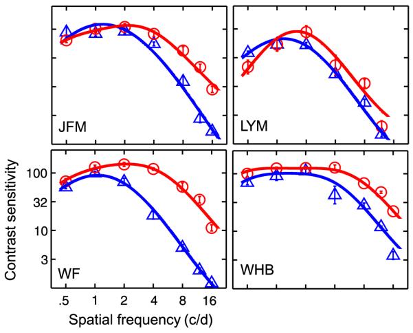
Contrast sensitivity functions for four amblyopic observers. Blue (amblyopic eye) and red (fellow eye) solid curves represent the predictions of the best fitting DOG functions.

The measured PvR functions for all five amblyopic observers are shown in Figures 6 and 7. Observer CCK ran the experiment twice, with a wider range of contrast ratio conditions in the second time (Figure 7). His data are labeled as CCK1 and CCK2. In both figures, the three columns represent three different base contrast conditions: 16%, 32% and 64%. The attenuation model with two parameters γ and η accounted for 97.1%, 99.3%, 97.9%, 99.6%, 96.1%, and 98.9% of the variance for CCK1, JFM, LYM, WF, WHB, and CCK2 respectively. For all amblyopic observers, the attenuation model provided significantly better fit to the data than the original Ding-Sperling model (all p < 0.0001).

Figure 6.

The phase versus interocular contrast ratio (PvR) functions for the amblyopic observers. Each panel shows the PvR functions in three phase difference conditions: 45 (red circle), 90 (green square) and 135 (blue triangles) degrees for a particular base contrast. Data from different base contrast conditions are shown in separate panels. Smooth curves represent predictions of the best fitting attenuation model.

Figure 7.

The phase versus interocular contrast ratio (PvR) functions for the second run of CCK with a wider range of interocular contrast ratios. Each panel shows PvR functions in three phase difference conditions: 45 (red circle), 90 (green square) and 135 (blue triangles) degrees for a particular base contrast. Data from different base contrast conditions are shown in separate panels: left, 0.16; middle, 032; right, 0.64. Smooth curves represent predictions of the best fitting attenuation model.

The predictions of the best fitting attenuation model are plotted as smooth curves in Figures 6 and 7. The average effective contrast ratios of the amblyopic eye (relative to the fellow eye) are 0.28 ± 0.01 for CCK1, 0.11 ± 0.01 for JFM, 0.21 ± 0.01 for LYM, 0.21 ± 0.01 for WF, 0.25 ± 0.01 for WHB, and 0.24 ± 0.01 for CCK2. These results indicate that the effective contrast in the amblyopic eye is much lower than that in the fellow eye during binocular combination. For the four observers with CSF data, the effective contrast ratios in binocular combination are much lower than their contrast sensitivity ratios (0.11 vs. 1.30, 0.21 vs. 1.42, 0.21 vs. 0.77, and 0.25 vs. 0.73, all p < 0.01).

Statistical comparisons of the various forms of the inhibition model generated the following results: The model in which the contrast-gain of the amblyopic eye is equal to the gain of the contrast gain in the fellow eye, i.e., α = β, provided statistically equivalent fits to the data as the full inhibition model (Table 3). For all five observers, the model in which the fellow eye only exerts stronger gain on the gain-control in the fellow eye but not on the gain-control on the amblyopic eye (α = 1) is inferior to the full inhibition model (all p < 0.01). For observers JFM, LYM and WHB, the model in which the fellow eye only exerts stronger gain-control on the amblyopic eye but not on the gain of the gain-control in the fellow eye (β = 1)is also inferior to the full inhibition model (all p < 0.01). The overall pattern of results suggest that the model in which α = β is the best fitting inhibition model. This model accounts for 97.9%, 99.3%, 98.3%, 99.7%, 97.2%, and 99.2% of the variance for CCK1, JFM, LYM, WF, WHB, and CCK2, respectively.

Table 3.

Parameters of the best-fitting inhibition model.

	CCK1	JFM	LYM	WF	WHB	CCK2*
γ	0.73	1.46	1.03	0.59	0.33	0.415
α	5.30	228.42	23.77	11.98	6.87	9.24
β	5.30	228.42	23.77	11.98	6.87	9.24
r 2	0.979	0.993	0.983	0.997	0.972	0.992
Fα = β(1,104)	1.11	0.07	2.89	0.18	1.99	2.50
Fβ = 1(1,104)	0.05	51.30	22.47	0.31	23.19	1.83
Fα = 1(1,104)	530.50	6626.80	2047.10	5847.40	685.05	2732.30

Note: The F-values represent statistics resulted from comparing the full inhibition model with the three less saturated inhibition models.

^*For CCK2, the degree of freedom of the F-tests is (1, 236).

Because the attenuation model and the best fitting α = β inhibition model are mathematically equivalent in predicting the perceived phase of the cyclopean image (Appendix B), we cannot distinguish the two potential mechanisms underlying abnormal binocular combination in amblyopia based on the data in this study. We can however treat the effective contrast ratio as an empirical measure of the imbalance of the contributions of the two eyes in binocular combination in amblyopic vision.

Discussion

By measuring the phase shift versus interocular contrast ratio functions, we found that both eyes contributed equally to binocular combination for observers with normal vision. However, for amblyopic observers, stimulus of equal contrast was weighted much less in the amblyopic eye relative to the fellow eye. For the five amblyopes, the effective contrast of the amblyopic eye in binocular combination is equal to about 11%–28% of the same contrast presented to the fellow eye, much less than the contrast sensitivity ratios between the amblyopic and fellow eyes (0.73 to 1.42).

One potential technical concern with the current study is related to phase perception in anisometropic amblyopia. Lawden et al. (1982) found that at medium to high spatial frequencies, many amblyopes demonstrated abnormality in phase discrimination. Pass and Levi (1982) obtained similar results using a ramp-wave stimulus. To avoid this potential problem, we used low spatial frequency, high contrast sine-wave gratings in this study. In fact, Lawden et al. (1982) found essentially normal phase discrimination in amblyopia when the gratings were of high contrasts and low spatial frequencies. Using direct phase discrimination measurements, Mac Cana et al. (1986) also found that the difference in phase discrimination between normal and amblyopic eyes was greatly reduced when tested with stimuli of low spatial frequency (1.33 c/deg), and concluded that the relatively poor phase discrimination observed in amblyopia reflected, at least in part, a deficit in contrast-coding. To control for potential phase discrimination deficits in the amblyopic eye, we also conducted a direct phase judgment test in the amblyopic eyes—when the interocular contrast ratio was zero, the phase of the cyclopean image was determined by the input from only one eye. As shown in Figures 4, 6, and 7, phase perception was essentially normal in the amblyopic eye tested in this study.

On the surface, our finding of lower effective contrast in the amblyopic eye in binocular combination seems to contradict the results of many studies in the literature that have demonstrated normal or near normal supra-threshold contrast perception in the amblyopic eye in anisometropic amblyopia (Hess & Bradley, 1980; Hess et al., 1983; Loshin & Levi, 1983). In fact, for all four amblyopic observers with available contrast sensitivity information, we found that the effective contrast ratios in binocular combination are much lower than the contrast sensitivity ratios between the amblyopic and fellow eyes. There are two possibilities: (1) Contrast perception (appearance) and binocular combination are two independent processes; Veridical contrast perception in the amblyopic eye may not necessarily guarantee equal effectiveness in binocular combination (Blaser, Sperling, & Lu, 1999); contrast in the amblyopic eye is attenuated during binocular combination. (2) Contrast in the amblyopic eye is as effective as that in the fellow eye. There is however stronger inhibition from the fellow eye to the amblyopic eye. Unfortunately, the best fitting inhibition model, in which the contrast-gain of the amblyopic eye is equal to the gain of the contrast gain in the fellow eye (α = β), is however mathematically equivalent to the attenuation model in determining the phase of the cyclopean images (Appendix B). Although we are aware that Baker et al. (2008) concluded that strabismic amblyopia attenuates the signal and increases internal noise in the amblyopic eye, we are at present uncommitted to either the attenuation or asymmetric inhibition theory in anisometropic amblyopia. We are conducting new studies to further test the two hypotheses.

Although we cannot discriminate the attenuation and the inhibition models, the PvR functions allow us to estimate the effective contrast ratio of the amblyopic eye in binocular combination. Estimating the effective contrast ratio in binocular combination is of great importance in amblyopia research. First, studies in normal subjects have found that stereoacuity depends on the contrast ratio of the inputs to the two eyes (Halpern & Blake, 1988; Legge & Gu, 1989). To obtain “true” measures of stereoacuity of amblyopes, we must equate the effective contrasts of the two eyes. The paradigm developed in this article makes it possible to measure and equate the effective contrasts of the two eyes in suprathreshold vision. Second, a number of studies showed that perceptual learning could improve contrast sensitivity in the amblyopic eye (Huang, Zhou, & Lu, 2008; Polat, Ma-Naim, Belkin, & Sagi, 2004; Zhou et al., 2006). Can improvements in contrast sensitivity increase the effective contrast ratio of the amblyopic eye in binocular combination and therefore improve stereoacuity? We are currently exploring these questions.

Appendix A

The contrast-gain control model for normals

In the contrast-gain control model of Ding and Sperling (2006) for normal observers (Figure 3a), the summed cyclopean image of the left (Lum_L) and right (Lum_R) eye inputs defined by Equations 1 and 2 is:

$${\mathrm{Lum}}^{\prime }=\frac{1}{1+\frac{{\epsilon }_R}{1+{\epsilon }_L}}{\mathrm{Lum}}_L+\frac{1}{1+\frac{{\epsilon }_L}{1+{\epsilon }_R}}{\mathrm{Lum}}_R,$$ (A1)

where ε_L and ε_R are the contrast energies presented to the two eyes and can be simply expressed as ε_L = ρ(C_L)^γ and ε_R = ρ(C_R)^γ, ρ is the gain-control efficiency of the signal sine-wave grating; γ is the exponent of the non-linearity. The contrast energies ε_L and ε_R are generally much greater than 1.0 even for the lowest contrast stimulus. We thus dropped the term “1” in Equation A1 in all the subsequent model development. For the four configurations illustrated in Figure 2, the phase shifts in the cyclopean images are:

$$\begin{array}{cc}\hfill & {\varphi }_a={\tan }^{-1}\left[\frac{1-{\delta }^{1+\gamma }}{1+{\delta }^{1+\gamma }}\tan \left(\frac{\theta }{2}\right)\right],\hfill \\ \hfill & {\varphi }_c=-{\tan }^{-1}\left[\frac{1-{\delta }^{1+\gamma }}{1+{\delta }^{1+\gamma }}\tan \left(\frac{\theta }{2}\right)\right],\hfill \end{array}$$ (A2)

$$\begin{array}{cc}\hfill & {\varphi }_b={\tan }^{-1}\left[\frac{1-{\delta }^{1+\gamma }}{1+{\delta }^{1+\gamma }}\tan \left(\frac{\theta }{2}\right)\right],\hfill \\ \hfill & {\varphi }_d=-{\tan }^{-1}\left[\frac{1-{\delta }^{1+\gamma }}{1+{\delta }^{1+\gamma }}\tan \left(\frac{\theta }{2}\right)\right],\hfill \end{array}$$ (A3)

To cancel possible up/down location bias and modest ocular dominance, we define two composite measures:

$${\varphi }_A={\varphi }_a-{\varphi }_c=2{\tan }^{-1}\left[\frac{1-{\delta }^{1+\gamma }}{1+{\delta }^{1+\gamma }}\tan \left(\frac{\theta }{2}\right)\right],$$ (A4)

$${\varphi }_F={\varphi }_b-{\varphi }_d=2{\tan }^{-1}\left[\frac{1-{\delta }^{1+\gamma }}{1+{\delta }^{1+\gamma }}\tan \left(\frac{\theta }{2}\right)\right],$$ (A5)

It is obvious that ϕ_A = ϕ_F. We keep them separate in order to be consistent with Appendix B.

In Equations A4 and A5, the perceived phase of the cyclopean image is determined by a single parameter, γ. Strictly speaking, ϕ_A and ϕ_F are not the perceived phase in any one of the four configurations in Figure 2. Rather, they are the difference between the phases of the cyclopean images of each pair of configurations. They have the following properties:

1. when the sine-wave in one eye is absent (δ = 0), the perceived phase of the cyclopean image is equal to that of the sine-wave in the other eye (ϕ_A = θ; ϕ_F = θ); and

2. when the amplitudes of the sine-waves in the two eyes are equal (δ = 1), the perceived phase of the cyclopean image is equal to zero (ϕ_A =0; ϕ_F = 0).

Appendix B

Contrast-gain control models in amblyopia

To construct models of cyclopean combination in amblyopia, we first re-write Equation A1 for amblyopic and fellow eyes:

$${\mathrm{Lum}}^{\prime }=\frac{1}{1+\frac{{\epsilon }_{F1}}{1+{\epsilon }_A}}{\mathrm{Lum}}_A+\frac{1}{1+\frac{{\epsilon }_A}{1+{\epsilon }_{F2}}}{\mathrm{Lum}}_F,$$ (B1)

where subscripts A and F stand for the amblyopic and fellow eyes, respectively. Again, we dropped the term “1” in Equation B1 in all the subsequent model development. We considered two ways to elaborate the Ding-Sperling model:

1. Attenuation in the amblyopic eye (Figure 3b): The effective contrast in the amblyopic eye is equal to its physical contrast multiplied by a factor η < 1, i.e., ε_A = ρ(ηC_A)^γ, ε_F1 = ε_F2 = ρ_CF^γ, and

2. Increased inhibition from the fellow eye (Figure 3c): All the contrast-gain control terms originated from the fellow eye are multiplied by factors greater than 1 in Equation B1, i.e., ε_A = ρ(C_A)^γ, ε_F1 = αρC_F^γ, ε_F2 = βρC_F^γ, with α > 1 and/or β > 1.

C_A and C_F represent image contrasts in the amblyopic and fellow eyes, respectively. We describe the two models in turn.

The attenuation model

If we treat the left eye as the amblyopic eye and the right eye as the fellow eye in Figure 2, the perceived phase of the cyclopean image for the four configurations are:

$$\begin{array}{cc}\hfill & {\varphi }_a={\tan }^{-1}\left[\frac{{\eta }^{1+\gamma }-{\delta }^{1+\gamma }}{{\eta }^{1+\gamma }+{\delta }^{1+\gamma }}\tan \left(\frac{\theta }{2}\right)\right],\hfill \\ \hfill & {\varphi }_c=-{\tan }^{-1}\left[\frac{{\eta }^{1+\gamma }-{\delta }^{1+\gamma }}{{\eta }^{1+\gamma }+{\delta }^{1+\gamma }}\tan \left(\frac{\theta }{2}\right)\right],\hfill \end{array}$$ (B2)

$$\begin{array}{cc}\hfill & {\varphi }_b={\tan }^{-1}\left[\frac{1-{\left(\eta \delta \right)}^{1+\gamma }}{1+{\left(\eta \delta \right)}^{1+\gamma }}\tan \left(\frac{\theta }{2}\right)\right],\hfill \\ \hfill & {\varphi }_d=-{\tan }^{-1}\left[\frac{1-{\left(\eta \delta \right)}^{1+\gamma }}{1+{\left(\eta \delta \right)}^{1+\gamma }}\tan \left(\frac{\theta }{2}\right)\right].\hfill \end{array}$$ (B3)

Following Ding and Sperling (2006), when a sine-wave grating with base contrast C₀ is presented to the amblyopic eye and a sine-wave grating with contrast δC₀ is presented to the fellow eye (Figures 2a and 2c), the perceived phase shift of the cyclopean image is:

$${\varphi }_A={\varphi }_a-{\varphi }_c=2{\tan }^{-1}\left[\frac{{\eta }^{1+\gamma }-{\delta }^{1+\gamma }}{{\eta }^{1+\gamma }+{\delta }^{1+\gamma }}\tan \left(\frac{\theta }{2}\right)\right].$$ (B4)

When a sine-wave grating with base contrast C₀ is presented to the fellow eye and a sine-wave grating with contrast δC₀ is presented to the amblyopic eye (Figures 2b and 2d), the perceived phase shift of the cyclopean image is:

$${\varphi }_F={\varphi }_b-{\varphi }_d=2{\tan }^{-1}\left[\frac{1-{\left(\eta \delta \right)}^{1+\gamma }}{1+{\left(\eta \delta \right)}^{1+\gamma }}\tan \left(\frac{\theta }{2}\right)\right].$$ (B5)

Both Equations B4 and B5 has the following properties:

1. when the sine-wave in one eye is absent (δ = 0), the perceived phase of the cyclopean image is equal to that of the sine-wave in the other eye (ϕ_A = θ; ϕ_F = θ); and

2. when the effective contrasts of the two eyes are equal (δ = η in Equation B4, or δ =1/η in Equation B5), the perceived phase of the cyclopean image is equal to zero (ϕ_A = 0; ϕ_F = 0).

In the attenuation model, PvR functions are completely determined by two parameters, γ and η.

The inhibition model

Following the same logic we used to derive Equations B4 and B5, we can obtain predictions of the inhibition model. When a sine-wave grating with base contrast C₀ is presented to the amblyopic eye and a sine-wave grating with contrast δC₀ is presented to the fellow eye (Figures 2a and 2c), the perceived phase shift of the cyclopean image is:

$${\varphi }_A={\varphi }_a-{\varphi }_c=2{\tan }^{-1}\left[\frac{\frac{1+\beta {\delta }^{\gamma }}{\beta (1+\alpha {\delta }^{\gamma })}-{\delta }^{1+\gamma }}{\frac{1+\beta {\delta }^{\gamma }}{\beta (1+\alpha {\delta }^{\gamma })}+{\delta }^{1+\gamma }}\tan \left(\frac{\theta }{2}\right)\right].$$ (B6)

When a sine-wave grating with base contrast C₀ is presented to the fellow eye and a sine-wave grating with contrast δC₀ is presented to the amblyopic eye (Figures 2b and 2d), the perceived phase shift of the cyclopean image is:

$${\varphi }_F={\varphi }_b-{\varphi }_d=2{\tan }^{-1}\left[\frac{\frac{\beta (\alpha +{\delta }^{\gamma })}{\beta +{\delta }^{\gamma }}-{\delta }^{1+\gamma }}{\frac{\beta (\alpha +{\delta }^{\gamma })}{\beta +{\delta }^{\gamma }}+{\delta }^{1+\gamma }}\tan \left(\frac{\theta }{2}\right)\right].$$ (B7)

In the inhibition model, PvR functions are completely determined by three parameters, α, β, and γ. We next consider three special cases:

1. The contrast-gain of the amblyopic eye (ε_F1) is equal to the gain of the contrast gain in the fellow eye (ε_F2), or equivalently, α = β. From Equations B6 and B7, we have

   $${\varphi }_A=2{\tan }^{-1}\left[\frac{1-\alpha {\delta }^{1+\gamma }}{1+\alpha {\delta }^{1+\gamma }}\tan \left(\frac{\theta }{2}\right)\right],$$ (B8)

   $${\varphi }_F=2{\tan }^{-1}\left[\frac{\alpha -{\delta }^{1+\gamma }}{\alpha +{\delta }^{1+\gamma }}\tan \left(\frac{\theta }{2}\right)\right].$$ (B9)

   If we let α = η^−(1+γ), Equations B8 and B9 are equivalent to Equations B4 and B5. In other words, attenuating the contrast in the amblyopic eye is mathematically equivalent to increasing the inhibition from the fellow eye in determining the phase of the cyclopean images if the strengths of the increased inhibitions are the same in the two gain-control paths.

2. The fellow eye only exerts stronger gain-control (ε_F1) on the amblyopic eye, not the gain of the gain-control in the fellow eye (ε_F2), i.e., β = 1. From Equations B6 and B7, we have:

   $${\varphi }_A=2{\tan }^{-1}\left[\frac{\frac{1+{\delta }^{\gamma }}{1+\alpha {\delta }^{\gamma }}-{\delta }^{1+\gamma }}{\frac{1+{\delta }^{\gamma }}{1+\alpha {\delta }^{\gamma }}+{\delta }^{1+\gamma }}\tan \left(\frac{\theta }{2}\right)\right],$$ (B10)

   $${\varphi }_F=2{\tan }^{-1}\left[\frac{\frac{\alpha +{\delta }^{\gamma }}{1+{\delta }^{\gamma }}-{\delta }^{1+\gamma }}{\frac{\alpha +{\delta }^{\gamma }}{1+{\delta }^{\gamma }}+{\delta }^{1+\gamma }}\tan \left(\frac{\theta }{2}\right)\right].$$ (B11)
3. The fellow eye only exerts stronger gain on the gain-control in the fellow eye (ε_F2), not gain-control on the amblyopic eye (ε_F1), i.e., α = 1. From Equations B6 and B7, we have:

   $${\varphi }_A=2{\tan }^{-1}\left[\frac{\frac{1+\beta {\delta }^{\gamma }}{\beta (1+{\delta }^{\gamma })}-{\delta }^{1+\gamma }}{\frac{1+\beta {\delta }^{\gamma }}{\beta (1+{\delta }^{\gamma })}+{\delta }^{1+\gamma }}\tan \left(\frac{\theta }{2}\right)\right],$$ (B12)

   $${\varphi }_F=2{\tan }^{-1}\left[\frac{\frac{\beta (1+{\delta }^{\gamma })}{\beta +{\delta }^{\gamma }}-{\delta }^{1+\gamma }}{\frac{\beta (1+{\delta }^{\gamma })}{\beta +{\delta }^{\gamma }}+{\delta }^{1+\gamma }}\tan \left(\frac{\theta }{2}\right)\right].$$ (B13)

References

- Agrawal R, Conner IP, Odom JV, Schwartz TL, Mendola JD. Relating binocular and monocular vision in strabismic and anisometropic amblyopia. Archives of Ophthalmology. 2006;124:844–850. doi: 10.1001/archopht.124.6.844. [PubMed] [Article] [DOI] [PubMed] [Google Scholar]
- Baker DH, Meese TS, Hess RF. Contrast masking in strabismic amblyopia: Attenuation, noise, interocular suppression and binocular summation. Vision Research. 2008;48:1625–1640. doi: 10.1016/j.visres.2008.04.017. [PubMed] [DOI] [PubMed] [Google Scholar]
- Baker DH, Meese TS, Mansouri B, Hess RF. Binocular summation of contrast remains intact in strabismic amblyopia. Investigative Ophthalmology & Visual Science. 2007;48:5332–5338. doi: 10.1167/iovs.07-0194. [PubMed] [Article] [DOI] [PubMed] [Google Scholar]
- Blaser E, Sperling G, Lu ZL. Measuring the amplification of attention. Proceedings of the National Academy of Sciences of the United States of America; 1999. pp. 11681–11686. [PubMed] [Article] [DOI] [PMC free article] [PubMed] [Google Scholar]
- Bonneh YS, Sagi D, Polat U. Local and non-local deficits in amblyopia: Acuity and spatial interactions. Vision Research. 2004;44:3099–3110. doi: 10.1016/j.visres.2004.07.031. [PubMed] [DOI] [PubMed] [Google Scholar]
- Bonneh YS, Sagi D, Polat U. Spatial and temporal crowding in amblyopia. Vision Research. 2007;47:1950–1962. doi: 10.1016/j.visres.2007.02.015. [PubMed] [DOI] [PubMed] [Google Scholar]
- Bradley A, Freeman RD. Contrast sensitivity in anisometropic amblyopia. Investigative Ophthalmology & Visual Science. 1981;21:467–476. [PubMed] [Article] [PubMed] [Google Scholar]
- Brainard DH. The Psychophysics Toolbox. Spatial Vision. 1997;10:433–436. [PubMed] [PubMed] [Google Scholar]
- Ciuffreda KJ, Levi DM, Selenow A. Amblyopia: Basic and clinical aspects. Butterworth-Heinemann; Boston: 1991. [Google Scholar]
- Daw NW. Critical periods and amblyopia. Archives of Ophthalmology. 1998;116:502–505. doi: 10.1001/archopht.116.4.502. [PubMed] [DOI] [PubMed] [Google Scholar]
- Ding J, Sperling G. A gain-control theory of binocular combination. Proceedings of the National Academy of Sciences of the United States of America; 2006. pp. 1141–1146. [PubMed] [Article] [DOI] [PMC free article] [PubMed] [Google Scholar]
- Ding J, Sperling G. Binocular combination: Measurements and a model. In: Harris L, Jenkin M, editors. Computational vision in neural and machine systems. Cambridge University Press; Cambridge, UK: 2007. pp. 257–305. [Google Scholar]
- Donzis PB, Rappazzo JA, Burde RM, Gordon M. Effect of binocular variations of Snellen’s visual acuity on Titmus stereoacuity. Archives of Ophthalmology. 1983;101:930–932. doi: 10.1001/archopht.1983.01040010930016. [PubMed] [DOI] [PubMed] [Google Scholar]
- Dudley LP. Stereoptics: An introduction. MacDonald & Co.; London: 1951. [Google Scholar]
- Flynn JT, McKenney SG, Dannheim E. Brightness matching in strabismic amblyopia. American Orthoptic Journal. 1971;21:38–49. [PubMed] [PubMed] [Google Scholar]
- Goodwin RT, Romano PE. Stereoacuity degradation by experimental and real monocular and binocular amblyopia. Investigative Ophthalmology & Visual Science. 1985;26:917–923. [PubMed] [Article] [PubMed] [Google Scholar]
- Halpern DL, Blake RR. How contrast affects stereoacuity. Perception. 1988;17:483–495. doi: 10.1068/p170483. [PubMed] [DOI] [PubMed] [Google Scholar]
- Harrad R, Sengpiel F, Blakemore C. Physiology of suppression in strabismic amblyopia. British Journal of Ophthalmology. 1996;80:373–377. doi: 10.1136/bjo.80.4.373. [PubMed] [Article] [DOI] [PMC free article] [PubMed] [Google Scholar]
- Harrad RA, Hess RF. Binocular integration of contrast information in amblyopia. Vision Research. 1992;32:2135–2150. doi: 10.1016/0042-6989(92)90075-t. [PubMed] [DOI] [PubMed] [Google Scholar]
- Harwerth RS, Levi DM. Psychophysical studies on the binocular processes of amblyopes. American Journal of Optometry and Physiological Optics. 1983;60:454–463. doi: 10.1097/00006324-198306000-00006. [PubMed] [DOI] [PubMed] [Google Scholar]
- Hess RF, Bradley A. Contrast perception above threshold is only minimally impaired in human amblyopia. Nature. 1980;287:463–464. doi: 10.1038/287463a0. [PubMed] [DOI] [PubMed] [Google Scholar]
- Hess RF, Bradley A, Piotrowski L. Contrast-coding in amblyopia. I. Differences in the neural basis of human amblyopia. Proceedings of the Royal Society of London B: Biological Sciences; 1983. pp. 309–330. [PubMed] [DOI] [PubMed] [Google Scholar]
- Hess RF, Howell ER. The threshold contrast sensitivity function in strabismic amblyopia: Evidence for a two type classification. Vision Research. 1977;17:1049–1055. doi: 10.1016/0042-6989(77)90009-8. [PubMed] [DOI] [PubMed] [Google Scholar]
- Hess RF, McIlhagga W, Field DJ. Contour integration in strabismic amblyopia: The sufficiency of an explanation based on positional uncertainty. Vision Research. 1997;37:3145–3161. doi: 10.1016/s0042-6989(96)00281-7. [PubMed] [DOI] [PubMed] [Google Scholar]
- Holopigian K, Blake R, Greenwald MJ. Selective losses in binocular vision in anisometropic amblyopes. Vision Research. 1986;26:621–630. doi: 10.1016/0042-6989(86)90010-6. [PubMed] [DOI] [PubMed] [Google Scholar]
- Holopigian K, Blake R, Greenwald MJ. Clinical suppression and amblyopia. Investigative Ophthalmology & Visual Science. 1988;29:444–451. [PubMed] [Article] [PubMed] [Google Scholar]
- Hood AS, Morrison JD. The dependence of binocular contrast sensitivities on binocular single vision in normal and amblyopic human subjects. The Journal of Physiology. 2002;540:607–622. doi: 10.1113/jphysiol.2001.013420. [PubMed] [Article] [DOI] [PMC free article] [PubMed] [Google Scholar]
- Howard IP, Rogers BJ. Binocular vision and stereopsis. Oxford University Press; New York: 1995. [Google Scholar]
- Huang CB, Zhou Y, Lu ZL. Broad bandwidth of perceptual learning in the visual system of adults with anisometropic amblyopia. Proceedings of the National Academy of Sciences of the United States of America; 2008. pp. 4068–4073. [PubMed] [Article] [DOI] [PMC free article] [PubMed] [Google Scholar]
- Jones RK, Lee DN. Why two eyes are better than one: The two views of binocular vision. Journal of Experimental Psychology: Human Perception and Performance. 1981;7:30–40. doi: 10.1037//0096-1523.7.1.30. [PubMed] [DOI] [PubMed] [Google Scholar]
- Kelly SL, Buckingham TJ. Movement hyperacuity in childhood amblyopia. British Journal of Ophthalmology. 1998;82:991–995. doi: 10.1136/bjo.82.9.991. [PubMed] [Article] [DOI] [PMC free article] [PubMed] [Google Scholar]
- Kiorpes L, McKee SP. Neural mechanisms underlying amblyopia. Current Opinion in Neuro-biology. 1999;9:480–486. doi: 10.1016/s0959-4388(99)80072-5. [PubMed] [DOI] [PubMed] [Google Scholar]
- Kiorpes L, Tang C, Movshon JA. Factors limiting contrast sensitivity in experimentally amblyopic macaque monkeys. Vision Research. 1999;39:4152–4160. doi: 10.1016/s0042-6989(99)00130-3. [PubMed] [DOI] [PubMed] [Google Scholar]
- Koskela PU, Hyvärinen L. Contrast sensitivity in amblyopia. IV. Assessment of vision using vertical and horizontal gratings and optotypes at different contrast levels. Acta Ophthalmologica. 1986;64:570–577. doi: 10.1111/j.1755-3768.1986.tb06975.x. [PubMed] [DOI] [PubMed] [Google Scholar]
- Lawden MC, Hess RF, Campbell FW. The discriminability of spatial phase relationships in amblyopia. Vision Research. 1982;22:1005–1016. doi: 10.1016/0042-6989(82)90037-2. [PubMed] [DOI] [PubMed] [Google Scholar]
- Legge GE, Gu YC. Stereopsis and contrast. Vision Research. 1989;29:989–1004. doi: 10.1016/0042-6989(89)90114-4. [PubMed] [DOI] [PubMed] [Google Scholar]
- Lema SA, Blake R. Binocular summation in normal and stereoblind humans. Vision Research. 1977;17:691–695. doi: 10.1016/s0042-6989(77)80004-7. [PubMed] [DOI] [PubMed] [Google Scholar]
- Levi DM, Hariharan S, Klein SA. Suppressive and facilitatory spatial interactions in amblyopic vision. Vision Research. 2002;42:1379–1394. doi: 10.1016/s0042-6989(02)00061-5. [PubMed] [DOI] [PubMed] [Google Scholar]
- Levi DM, Harwerth RS. Contrast evoked potentials in strabismic and anisometropic amblyopia. Investigative Ophthalmology & Visual Science. 1978;17:571–575. [PubMed] [Article] [PubMed] [Google Scholar]
- Levi DM, Harwerth RS, Manny RE. Suprathreshold spatial frequency detection and binocular interaction in strabismic and anisometropic amblyopia. Investigative Ophthalmology & Visual Science. 1979;18:714–725. [PubMed] [Article] [PubMed] [Google Scholar]
- Levi DM, Harwerth RS, Smith EL. Binocular interactions in normal and anomalous binocular vision. Documenta Ophthalmologica. 1980;49:303–324. doi: 10.1007/BF01886623. [PubMed] [DOI] [PubMed] [Google Scholar]
- Levi DM, Klein S. Hyperacuity and amblyopia. Nature. 1982;298:268–270. doi: 10.1038/298268a0. [PubMed] [DOI] [PubMed] [Google Scholar]
- Levi DM, Li RW, Klein SA. “Phase capture” in amblyopia: The influence function for sampled shape. Vision Research. 2005;45:1793–1805. doi: 10.1016/j.visres.2005.01.021. [PubMed] [DOI] [PubMed] [Google Scholar]
- Levitt H. Transformed up-down methods in psychoacoustics. Journal of the Acoustical Society of America. 1971;49:467–477. [PubMed] [PubMed] [Google Scholar]
- Li X, Lu ZL, Xu P, Jin J, Zhou Y. Generating high gray-level resolution monochrome displays with conventional computer graphics cards and color monitors. Journal of Neuroscience Methods. 2003;130:9–18. doi: 10.1016/s0165-0270(03)00174-2. [PubMed] [DOI] [PubMed] [Google Scholar]
- Loshin DS, Levi DM. Suprathreshold contrast perception in functional amblyopia. Documenta Ophthalmologica. 1983;55:213–236. doi: 10.1007/BF00140810. [PubMed] [DOI] [PubMed] [Google Scholar]
- Mac Cana F, Cuthbert A, Lovegrove W. Contrast and phase processing in amblyopia. Vision Research. 1986;26:781–789. doi: 10.1016/0042-6989(86)90093-3. [PubMed] [DOI] [PubMed] [Google Scholar]
- Maloney LT. Confidence intervals for the parameters of psychometric functions. Perception & Psychophysics. 1990;47:127–134. doi: 10.3758/bf03205977. [PubMed] [DOI] [PubMed] [Google Scholar]
- McKee SP, Levi DM, Movshon JA. The pattern of visual deficits in amblyopia. Journal of Vision. 2003;3(5):5, 380–405. doi: 10.1167/3.5.5. http://journalofvision.org/3/5/5/, doi:10.1167/3.5.5. [PubMed] [Article] [DOI] [PubMed] [Google Scholar]
- Meese TS, Georgeson MA, Baker DH. Binocular contrast vision at and above threshold. Journal of Vision. 2006;6(11):7, 1224–1243. doi: 10.1167/6.11.7. http://journalofvision.org/6/11/7/, doi:10.1167/6.11.7. [PubMed] [Article] [DOI] [PubMed] [Google Scholar]
- Mitchell DE, Reardon J, Muir DW. Interocular transfer of the motion after-effect in normal and stereoblind observers. Experimental Brain Research. 1975;22:163–173. doi: 10.1007/BF00237686. [PubMed] [DOI] [PubMed] [Google Scholar]
- Pardhan S, Gilchrist J. Binocular contrast summation and inhibition in amblyopia. The influence of the interocular difference on binocular contrast sensitivity. Documenta Ophthalmologica. 1992;82:239–248. doi: 10.1007/BF00160771. [PubMed] [DOI] [PubMed] [Google Scholar]
- Pass AF, Levi DM. Spatial processing of complex stimuli in the amblyopic visual system. Investigative Ophthalmology & Visual Science. 1982;23:780–786. [PubMed] [Article] [PubMed] [Google Scholar]
- Pelli DG. The VideoToolbox software for visual psychophysics: Transforming numbers into movies. Spatial Vision. 1997;10:437–442. [PubMed] [PubMed] [Google Scholar]
- Polat U, Ma-Naim T, Belkin M, Sagi D. Improving vision in adult amblyopia by perceptual learning. Proceedings of the National Academy of Sciences of the United States of America; 2004. pp. 6692–6697. [PubMed] [Article] [DOI] [PMC free article] [PubMed] [Google Scholar]
- Pratt-Johnson JA. Sensory phenomenon associated with suppression. British Orthoptic Journal. 1969;26:15–24. [Google Scholar]
- Pugh M. Foveal vision in amblyopia. British Journal of Ophthalmology. 1954;38:321–331. doi: 10.1136/bjo.38.6.321. [PubMed] [Article] [DOI] [PMC free article] [PubMed] [Google Scholar]
- Rohaly AM, Buchsbaum G. Inference of global spatiochromatic mechanisms from contrast sensitivity functions. Journal of the Optical Society of America A, Optics and Image Science. 1988;5:572–576. doi: 10.1364/josaa.5.000572. [PubMed] [DOI] [PubMed] [Google Scholar]
- Rohaly AM, Buchsbaum G. Global spatiochromatic mechanism accounting for luminance variations in contrast sensitivity functions. Journal of the Optical Society of America A, Optics and Image Science. 1989;6:312–317. doi: 10.1364/josaa.6.000312. [PubMed] [DOI] [PubMed] [Google Scholar]
- Sharma V, Levi DM, Klein SA. Under-counting features and missing features: Evidence for a high-level deficit in strabismic amblyopia. Nature Neuroscience. 2000;3:496–501. doi: 10.1038/74872. [PubMed] [DOI] [PubMed] [Google Scholar]
- Sheedy JE, Bailey IL, Buri M, Bass E. Binocular vs. monocular task performance. American Journal of Optometry and Physiological Optics. 1986;63:839–846. doi: 10.1097/00006324-198610000-00008. [PubMed] [DOI] [PubMed] [Google Scholar]
- Simmers AJ, Ledgeway T, Hess RF, McGraw PV. Deficits to global motion processing in human amblyopia. Vision Research. 2003;43:729–738. doi: 10.1016/s0042-6989(02)00684-3. [PubMed] [DOI] [PubMed] [Google Scholar]
- Walraven J, Janzen P. TNO stereopsis test as an aid to the prevention of amblyopia. Ophthalmic & Physiological Optics. 1993;13:350–356. doi: 10.1111/j.1475-1313.1993.tb00490.x. [PubMed] [DOI] [PubMed] [Google Scholar]
- Wheatstone C. Contributions to the physiology of vision—Part the first. On some remarkable, and hitherto unobserved. Phenomena of Binocular Vision. Royal Society of London, Philosophical Transactions. 1838;128:371–394. [Google Scholar]
- Wood IC, Fox JA, Stephenson MG. Contrast threshold of random dot stereograms in anisometropic amblyopia: A clinical investigation. British Journal of Ophthalmology. 1978;62:34–38. doi: 10.1136/bjo.62.1.34. [PubMed] [Article] [DOI] [PMC free article] [PubMed] [Google Scholar]
- Zhou Y, Huang C, Xu P, Tao L, Qiu Z, Li X, Lu Z-L. Perceptual learning improves contrast sensitivity and visual acuity in adults with anisome-tropic amblyopia. Vision Research. 2006;46:739–750. doi: 10.1016/j.visres.2005.07.031. [PubMed] [DOI] [PubMed] [Google Scholar]