

Abstract
We present the three-dimensional molecular theory of solvation (also known as 3D-RISM) coupled with molecular dynamics (MD) simulation by contracting solvent degrees of freedom, accelerated by extrapolating solvent-induced forces and applying them in large multi-time steps (up to 20 fs) to enable simulation of large biomolecules. The method has been implemented in the Amber molecular modeling package, and is illustrated here on alanine dipeptide and protein G.
1 Introduction
Molecular dynamics (MD) simulation with explicit solvent, in particular, available in the Amber molecular dynamics package,1 yields accurate and detailed modeling of biomolecules (e.g. proteins and DNA) in solution, provided the processes to be described are within accessible time scales, typically up to tens of nanoseconds. A major computational burden comes from the treatment of solvent molecules (usually water, sometimes cosolvent, and counterions/buffer or salt for electrolyte solutions) which typically constitute a large part of the system. Moreover, solvent enters pockets and inner cavities of the proteins through their conformational changes, which is a very slow process and nearly as difficult to model as protein folding.
Of no surprise, then, is the considerable interest in MD simulation with solvent degrees of freedom contracted by using implicit solvation approaches. In particular, the generalized Born (GB) model,2 in which the solvent polarization effects are represented by a cavity in dielectric continuum (optionally, with Debye screening by the charge distribution of structureless ions in the form of the Yukawa screened potential), whereas the non-electrostatic contributions are phenomenologically parameterized against the solvent accessible area and excluded volume of the biomolecule. The cavity shape is formed by rolling a spherical probe, of a size to be parameterized for each solvent, over the surface of the biomolecule. The polarization energy follows from the solution to the Poisson equation, which is computationally expensive, and is approximated in the GB model for fast calculation by algebraic expressions interpolating between the simple cases of two point charges in a spherical cavity. Conceptually transparent and computationally simple, the GB model has long been popular, including its implementations in the Amber molecular dynamics package.1 However, it bears the fundamental drawbacks of implicit solvation methods: the energy contribution from solvation shell features such as hydrogen bonding can be parameterized but not represented in a transferable manner; the three-dimensional variations of the solvation structure, in particular, the second solvation shell are lost; the volumetric properties of the solute are not well defined; the non-electrostatic solvation energy terms are empirically parameterized, and therefore, effective interactions like hydrophobic interaction and hydrophobic attraction are not described from the first principles and thus are not transferable to new systems with complex compositions (e.g. with cosolvent and/or different buffer ions); the entropic term is absent in continuum solvation, thus excluding from consideration the whole range of effects, such as the energy-entropy balance for the temperature control over supramolecular self-assembly in solution. To this end, the notion of a surface accessible surface, defined as that delineated by the center of the probe “rolled” over the surface becomes meaningless for inner cavities of biomolecules hosting just a few solvent molecules.
An attractive alternative to continuum solvation is the three-dimensional molecular theory of solvation, also known as the 3D reference interaction site model (3D-RISM).3–10 Starting from an explicit solvent model, it operates with solvent distributions rather than individual molecules, but yields the solvation structure and thermodynamics from the first principles of statistical mechanics. It properly accounts for chemical specificities of both solute and solvent molecules, such as hydrogen bonding or other association and hydrophobic forces, by yielding the 3D site density distributions of solvent, similar to explicit solvent simulations. Moreover, it readily provides via analytical expressions all the solvation thermodynamics, including the solvation free energy potential, its energetic and entropic decomposition, and partial molar volume and compressibility. The expression for the solvation free energy (and its derivatives) in terms of integrals of the correlation functions follows from a particular approximation for the so-called closure relation used to complete the integral equation for the direct and total correlation functions.11 The 3D-RISM theory in the so-called hypernetted chain (HNC) closure approximation was sketched by Chandler and co-workers in their derivation of density functional theory for classical site distributions of molecular liquids.3,4 Beglov and Roux for the first time used the 3D-HNC closure to calculate the distribution of a monoatomic Lennard-Jones (LJ) solvent in the neighborhood of solid substrates of arbitrary shape constructed from LJ centers12 and introduced the 3D-RISM-HNC theory in the above way for polar molecules in liquid water.5 Kovalenko and Hirata derived the 3D-RISM integral equation from the six-dimensional, molecular Ornstein-Zernike integral equation11 for the solute-solvent correlation functions by averaging out the orientation degrees of freedom of solvent molecules while keeping the orientation of the solute macromolecule described at the three-dimensional level.6,7,10 They also developed an analytical treatment of the electrostatic long-range asymptotics of both the 3D site direct correlation functions (Coulomb tales) and total correlation functions (screened Coulomb tales and constant shifts), including analytical corrections to the 3D site correlation functions for the periodicity of the supercell used in solving the 3D-RISM integral equation.8–10 This enabled 3D-RISM calculation of the solvation structure and thermodynamics of different ionic and polar macromolecules/supramolecules, for which distortion or loss of the long-range asymptotics of either of the correlation functions leads to huge errors in the 3D-RISM results for the solvation free energy (even for simple ions and ion pairs in water) while the analytical corrections/treatment of the asymptotics restores it to an accuracy of a small fraction of kcal/mol. Furthermore, Kovalenko and Hirata proposed the closure approximation (3D-KH closure) that couples the 3D-HNC treatment automatically applied to repulsive cores and other regions of density depletion due to repulsive interaction and steric constraints, and the 3D mean-spherical approximation (3D-MSA) applied to distribution peaks due to associative forces and other density enhancements, including long-range distribution tales for structural and phase transitions in fluids and mixtures.7,10 The 3D-KH approximation yields solutions to the 3D-RISM equations for polyionic macromolecules, solid-liquid interfaces, and fluid systems near structural and phase transitions, for which the 3D-HNC approximation is divergent and the 3D-MSA produces non-physical areas of negative density distributions. (For the site-site OZ, or conventional RISM theory,11 the corresponding radial 1D-KH version is available and capable of predicting phase and structural transitions in both simple and complex associating liquids and mixtures.10) The 3D-RISM-KH theory has been successful in analyzing a number of chemical and biological systems in solution,10 including structure of solid-liquid interfaces,7 structural transitions and thermodynamics of micromicelles in alcohol-water mixtures,13,14 structure and thermochemistry of various inorganic and (bio)organic molecules in different solvents,15,16 conformational equilibria, tautomerization energies, and activation barriers of chemical reactions in solution,16 solvation of carbon nanotubes,15 structure and thermodynamics of self-assembly, stability and conformational transitions of synthetic organic supramolecules (e.g. organic rosette nanotubes in different solvents)17–20 as well as peptides and proteins in aqueous solution,21–23 and molecular recognition and ligand-protein docking in solution.23,24 It constitutes a promising method to contract solvent degrees of freedom in MD simulation.
Miyata and Hirata25 have introduced a coupling of 3D-RISM with MD in a multiple time step (MTS) algorithm which can be formulated in terms of the RESPA26,27 method. It converges the 3D-RISM equations for the solvent correlations at the current snapshot of the solute conformation by using the accelerated iterative MDIIS solver, then performs several MD steps, and solves the 3D-RISM equations over again. The MDIIS (modified direct inversion in the iterative subspace) procedure10 is a Krylov subspace type iterative solver for integral equations of liquid state theory, closely related to the DIIS approach of Pulay28 for quantum chemistry equations and other similar algorithms, in particular, the GMRES solver.29 The MTS approach was necessary to bring down the relatively large computational expenses of solving the 3D-RISM equations. Their implementation achieved stable simulation with the 3D-RISM equations solved at each 5th step of MD at most, which is not sufficient for realistic simulation of macromolecules and biomolecular structures of interest.
In this work, we couple the 3D-RISM solvation theory with MD in the AMBER molecular dynamics package in an efficient way that includes a number of accelerating schemes. This includes several cutoffs for the interaction potentials and correlation functions, an iterative guess for the 3D-RISM solutions, and an MTS procedure with solvation forces at each MD step which are extrapolated from the previous 3D-RISM evaluations. This coupled method makes modeling of biomolecular structures of practical interest, e.g. proteins with water in inner pockets feasible. As a preliminary illustration, we apply the method to Alanine-dipeptide and protein G in ambient water.
2 Theory and Implementation
2.1 Molecular Solvation
Solvation free energies, and their associated forces, are obtained for the solute from the 3D reference interaction site model (3D-RISM) for molecular solvation, coupled with the 3D version of the Kovalenko-Hirata (3D-KH) closure.10 3D-RISM provides the solvent structure in the form of a 3D site distribution function, , for each solvent site, γ. With gγ (r) → 1, the solvent density distribution ργ (r) = ργgγ (r) approaches the solvent bulk density ργ. The 3D-RISM integral equation has the form
| (1) |
where superscripts ‘U’ and ‘V’ denote the solute and solvent species respectively; h (r) = g (r) − 1 is the site-site total correlation function; is the 3D direct correlation function for solvent site α having asymptotics of the interaction potential between the solute and solvent site: ; and is the site-site susceptibility of the solvent, given by
| (2) |
Here, is the intramolecular correlation function, representing the internal geometry of the solvent molecules while is the site-site radial total correlation function of the pure solvent calculated from the dielectrically consistent version of the 1D-RISM theory (DRISM).30,31 eq 1 is complemented with the 3D-KH closure
| (3) |
where
and is the 3D interaction potential of the solute acting on solvent site γ, given by the sum of the pairwise site-site potentials from all the solute interaction sites i located at frozen positions Ri,
| (4) |
As with the 3D-HNC closure approximation, the 3D-RISM eq 1 with 3D-KH closure (3) possesses an exact differential of the free energy, and thus has a closed analytical expression for the excess chemical potential of solvation10
| (5) |
where Θ(x) is the Heaviside function, which results in (hα(r))2 being applied only in areas of site density depletion.
2.2 Analytical Solvent Forces for 3D-RISM
The solvation free energy Δμ is generally determined by the Kirkwood “charging” formula with thermodynamic integration over the parameter λ gradually “switching on” the solute-solvent interaction potential ũ(r;λ) along some path from no interaction at λ = 0 to the full interaction potential u(r) at λ = 1. In the case of the interaction site model, it has the form
| (6) |
The solvation free energy Δμ({Ri}) dependent on protein conformation {Ri}, determined by (6) and obtained as (5) is actually the potential of mean force. The expression for the mean solvent force acting on each atom i of the solute is defined as a derivative of the solvation free energy with respect to the atom coordinates Ri. The mean solvent force can by obtained in the general form by differentiating the expression (6) modified in such a way that the thermodynamic integration is extended over the endpoint λ = 1 to the full interaction potential further changed by due to infinitesimal shift dRi of solute atom i,
For the 3D site interaction potential (4), differentiation of this expression with respect to Ri immediately gives the mean solvent force acting on solute site i as
| (7) |
where is the pairwise interaction potential between solute site i located at Ri and solvent site γ at r. It is obvious that the form (7) is valid for any closure approximation that yields the solvation free energy (at a frozen solute conformation {Ri}) independent on a thermodynamic integration path, that is, possesses an exact free energy differential. These are, in particular, the 3D-HNC and 3D-KH closures.10 The expression (7) has also been obtained, by directly differentiating a closure to the 3D-RISM equation, for the 3D-KH closure15 and for the 3D-HNC closure.15,25 The mean solvent force in the general form (7) still holds for any closure, subject to performing the thermodynamic integration along the path described above.
2.3 Computational Methods for Accelerating Dynamics
Modifications to the SANDER molecular dynamics module of Amber were minor. Other than calling the RISM3D subroutine, the only modifications were to add in calls for memory allocation and file input/output. A single 3D-RISM calculation is roughly three orders of magnitude slower than a single time step for a system solvated with the same solvent model at the same volume and density. This is not unexpected as 3D-RISM calculates the complete equilibrium distribution of solvent about the solute. To obtain meaningful sampling of solute conformations it is necessary to reduce the computational expense of 3D-RISM calculations. To achieve this goal three different optimization strategies were employed: (1) high quality initial guesses to the direct correlation function were created from multiple previous solutions; (2) the pre- and post-processing of the solute-solvent potentials, long-range asymptotics and forces was accelerated using a cut-off scheme and minimal solvation box; and (3) direct calculation of the 3D-RISM solvation forces was avoided altogether by interpolating current force based off of atom positions from previous time steps.
2.3.1 Solution Propagation
Rapid convergence of an individual 3D-RISM calculation is facilitated by a high quality initial guess. Given the nature of molecular dynamics simulations, it is possible to use solutions from previous time steps as the initial guess for current time step tk. The simplest case is to use the solution from the previous time step. It is possible to improve on this by including numerically calculated derivatives
| (8) |
Derivatives may be calculated for each point on the grid using finite difference techniques. In this paper we have used up to the fourth order derivative to calculate initial guess:
| (9) |
| (10) |
| (11) |
| (12) |
| (13) |
The order at which the propagation is terminated can be indicated by the number of previous solutions used, .
2.3.2 Adaptive Solvation Box
The number of floating point entries that must be stored in memory for a 3D-RISM calculation is approximately
| (14) |
where NFP is the total number of floating point entries, Nbox = Nx × Ny × Nz is the total number of grid points, Nsolv is the number of solvent atom species and NMDIIS is the number of MDIIS vectors used to accelerate convergence. A full grid for g and h is required for each solvent species and four grids are required to compute the long range asymptotics. Memory, therefore, scales linearly with Nbox while computation time scales as O(Nbox log(Nbox)) due to the requirements of calculating the 3D fast Fourier transform (3D-FFT).
For independent 3D-RISM calculations solvation box dimensions can be selected to accommodate the particular shape of the solute. For MD, however, a solvation box of fixed size through out the simulation must be cubic to accommodate rotations and large enough to handle changes in size and shape of the solute. Alternatively, the solvation box may be determined dynamically throughout the simulation. In this case, a linear grid spacing and minimal buffer distance between any atom of the solute and the edge of the solvent box is specified. The actual dimensions of the solvent box must satisfy the constraints of maintaining specified buffer distance and linear grid spacing. In order to calculate the required 3D-FFT and long range asymptotics each grid dimension must also be divisible by two and have factors of only two, three or five. Previous solutions may still be propagated by transferring the past solutions to the new grid. Past solutions are truncated or padded with zeroes as required by larger or small grid dimension.
2.3.3 Potential and Force Cut-offs
Both solute-solvent potential interactions and force calculations require interactions of every solute atom with every grid point for each solvent atom species. These calculations then scale as O(NboxMUMV) where MU and MV are the number of solute atoms and solvent species respectively. As each grid point must still be assigned a values, the use of cutoffs will not change how these calculations scale. However, computationally expensive distance-based potential calculations can be replaced with cheaper calculations outside the cut-off, reducing the computational cost by a constant factor.
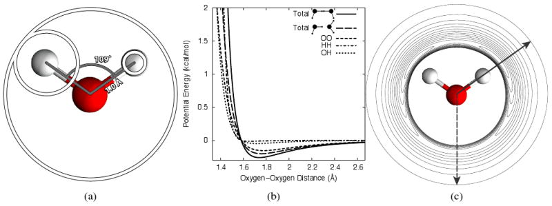
As Lennard-Jones and coulomb potentials have different long-range asymptotic behavior, the two potentials are treated differently outside the cut-off radius. Lennard-Jones calculations use a hard cut-off for each solute atom. For both potential and force calculations, each solute atom only interacts with grid points within the cut-off distance, as is depicted in Figure 1(a). In contrast, the long tail of the coulomb interaction does not allow hard cut-offs to be used. Rather, within the union of the entire volume within the cut-off distance of all atoms the entire interaction for all solute atoms is calculated at each grid point (see Figure 1(b)). Outside of this volume, where the interaction varies smoothly, only even grid points have the full potential calculated. I.e., only one eighth of the grid is visited. Values are then interpolated for grid points that have not been visited using a fast interpolation scheme.32
Figure 1.

Cut-off schemes for grid based (a) Lennard-Jones and (b) coulomb potential and force calculations. Lennard-Jones calculations are performed for each solute atom only at grid sites within the cut-off distance of that atom. Grid sites within the cut-off distance of multiple solute sites take on the sum of these interactions. Coulomb interactions are calculated for every solute atom at grid sites in the union of all cut-off volumes. Grid sites outside the cut-off use explicit calculations or interpolation from surrounding values.
Contributions to atomic forces from grid points outside the cut-off volume are calculated in an analogous treatment for both Lennard-Jones and coulomb interactions. For Lennard-Jones forces on each solute atom, only the volume within the cut-off distance from that atom is included in the integration. Coulomb forces achieve the same low density sampling used in the potential calculation by doubling the integration step size outside of the cut-off volume, effectively visiting only one eighth of the points in this region. However, for simplicity, the cut-off volume is taken as a rectangular prism rather than a sphere for coulomb forces alone.
An alternate method for the electrostatic potential is Ewald summation,33 which scales as O(Nbox ln(Nbox)MV). This scaling is generally better than the cut-off method with interpolation described as ln(Nbox) < MU for most systems. However, the scaling coefficients for the two methods are not equal and the cutoff method significantly outperformed Ewald summation for systems in this study. Furthermore, Ewald summation necessarily provides a periodic potential and a correction to this must be computed to maintain the assumption of infinite dilution,34 adding to the overhead of the Ewald method. Of course, for a large enough solute the Ewald method with periodic correction will be more efficient than the cutoff method.
2.3.4 Force Extrapolation
A variety of multiple time step (MTS) method have been developed to limit the number of expensive force calculations required for MD. Specifically for 3D-RISM-HNC calculations, Miyata and Hirata25 used RESPA MTS26,27 where slowly varying forces are only applied at an integer multiple of the base time step, effectively introducing large, periodic impulses to the dynamics. RESPA MTS has desirable properties, such as energy conservation, however, it is well known that resonance artifacts limit the MTS step size to 5 fs for atomistic biomolecular simulations, after which the method becomes catastrophically unstable.35–37 An alternate approach, extrapolative MTS, applies a constant force over all intermediate time steps. There are no impulses in this method to cause resonance artifacts but it does not conserve energy as the forces at intermediate time steps do not correspond to a conservative potential. LN MTS couples extrapolative MTS with Langevin dynamics to produce stable trajectories for MTS time steps up to 10s or 100s of femtoseconds, provided the forces being extrapolated are slow varying on these time scales.37–39 Unfortunately, the microscopic detail present in 3D-RISM calculations give rise to forces vary on too short a timescale to make use of LN MTS.
Inspired by LN MTS, we introduce force-coordinate extrapolation (FCE) MTS. Rather than applying a constant force, based on the last force calculations, we use previous atom configurations and forces to extrapolate what the forces should be at intermediate time steps. In this method, the forces on each of the MU solute atoms for a current intermediate time step tk given by the 3 × MU matrix of forces {F}(k) are approximated as a linear combination of forces {F}(l) at N previous time steps obtained in 3D-RISM calculations,
| (15) |
The weight coefficients akl are obtained as the best representation of the arrangement of solute atoms at the current time step k in terms of its projections onto the “basis” of N previous solute arrangements obtained from 3D-RISM, by minimizing the norm of the difference between the current 3 × MU matrix of coordinates {R}(k) and the corresponding linear combination of the previous ones {R}(l),
| (16) |
This is achieved by calculating the scalar products of the current coordinates matrix {R}(k) and each basis coordinates matrix {R}(l) and between all the basis matrices,
| (17) |
where i is the solute atom index, and then solving the set of N linear equations for the weight coefficients akl,
| (18) |
Coefficients akl′ are then used in eq 15 to extrapolate forces at the current intermediate time step. Similarly, the known coordinates for the current time step can be approximated from previous time steps as
| (19) |
These forces are approximate and do not correspond to a conservative potential; thus, MD simulations using these forces will not conserve energy. However, they provide ‘smooth’ transition between explicitly calculated forces. As in the LN MTS method, the resulting energy gains can be damped out with the use of Langevin dynamics to provide stable, constant temperature trajectories and enhance conformational sampling through increased efficiency.38,39
With this method one chooses a base time step, δt, and then calculates 3D-RISM at an integer number of base time steps, giving Δt between 3D-RISM calculations. Furthermore, RESPA MTS can also be applied to the intermediate, extrapolated forces, reducing the number of extrapolations required. As a concrete example, one can choose δt = 2 fs; after the specified number of previous coordinate sets with 3D-RISM forces has been calculated, extrapolated forces can be applied every 5 fs with new 3D-RISM solutions calculated every Δt = 20 fs.
Since the solvation forces on any particular solute atom typically correlate only with nearest neighbors, it is possible to use a cut-off for {R} and {F}. Given the size of the systems in this paper, this was not used though this capability is in our implementation.
2.3.5 Distributed Memory Parallelization
3D-RISM calculations typically require large amounts of both computer time and memory. A distributed memory parallel implementation allows computation time to be decreased but also allows the aggregate memory of a distributed cluster to be utilized. The role of 3D-FFTs in calculation 3D-RISM solutions dictates that the memory model of the 3D-FFT library must be adopted by 3D-RISM. As we use the FFTW 2.1.5 library,40 memory decomposition is performed along the Z-axis for all 3D arrays (uUV, gUV, hUV, cUV etc.). Communication between processes only occurs in the MDIIS, 3D-FFT routines and for the final summation of forces.
The force extrapolation method may also be parallelized. In anticipation of the use of cut-offs, coefficients for each solute atom in eq 19 are found independently. This is trivially distributed between processes.
2.4 Solvent Model
1D- and 3D-RISM calculate the equilibrium distribution of an explicit solvent model. Two of the most popular models for water, SPC/E41 and TIP3P,42 do not include van der Waals terms for the hydrogens. The incomplete intramolecular correlation in RISM theory allows a catastrophic overlap between oxygen and hydrogen sties, preventing 1D-RISM from converging on a solution. The standard approach to this problem has been to apply a small Lennard-Jones potential to the hydrogen atoms
| (20) |
Common parameters used in the literature include those of Pettitt and Rossky, σ = 0.4 Å and ε = 0.046 kcal/mol,43 which we will refer to as PR-SPC/E and PR-TIP3P, and those often used by Hirata and co-workers, σ = 1.0 Å and ε = 0.05455 kcal/mol.44 As noted by Sato and Hirata,45 van der Waals parameters are required to solve the RISM equations but also perturb the thermodynamics of the solution.
Alternative approaches to this problem do exist and involve corrective bridge functions46–48 or new formalisms that go beyond RISM theory to include orientational correlations and use proper diagrams.49–52 The major drawback of the corrective bridge function approach is that a new expression for the excess chemical potential must be derived, a non-trivial task. By including our correction in the potential, the standard closures and related thermodynamic expressions still hold. Including orientational correlations obviates the need for any “protective” Lennard-Jones potential and holds considerable promise. However, the computational complexity of these methods is even greater than that of RISM. Applying them to relatively simple systems presented here will require considerable further development of these methods.
To overcome shortcomings in previous Lennard-Jones parameters while maintaining an analytic expression for the excess chemical potential and mean solvation force, we introduce a general and transferable rule that can be applied to any model with embedded sites. Specifically, we choose
| (21) |
| (22) |
where σe is the radius of the embedded site, σh is the radius of the host site and bhe is the bond length between the two. As the embedded radius is now coincident with the host radius along the bond vector, unphysical overlap between sites is prevented. The size of εe relative to εh balances deforming the potential of the host while proving a “stiff” enough potential to the embedded site to prevent overlaps. When applied to SPC/E and TIP3P we refer to these models as coincident SPC/E (cSPC/E) and coincident TIP3P (cTIP3P). This is illustrated for SPC/E water in Figure 2(a) and parameters for SPC/E and TIP3P water are given in Table 1.
Figure 2.
Modified water potential. (a) Schematic illustration of Lennard-Jones parameters for SPC/E water. Lennard-Jones radii, σ/2, are illustrated by white circles. The radius on the right hand hydrogen corresponds to that of Pettitt and Rossky43 while the left hand hydrogen radius is from eqs 21 and 22. (b) Perturbation of water-water Lennard-Jones potential due to the hydrogen potential. The maximum perturbation (solid line) is for two waters with hydrogens aligned. The case of hydrogen bonding is given by the long-dashed line while the original potential is given by the short dashed line. HH (dot-dashed line) and OH (dotted line) interactions are a result of the new parameters. (c) Angle dependent water-water interaction. The second water is oriented such that a hydrogen is always pointing towards the central water. The solid and long dashed arrows correspond to the solid and long-dashed lines in (b). Contour lines are spaced 0.02 kcal/mol apart.
Table 1.
Parameters for standard and modified SPC/E and TIP3P water models.
| Model Name | σO | εO | σH | εH | qO | qH | r(OH) |
|---|---|---|---|---|---|---|---|
| Å | kcal/mol | Å | kcal/mol | e | Å | ||
| SPC/E | 3.1658 | 0.15530 | - | - | -0.8476 | 0.4238 | 1.0000 |
| cSPC/E | 3.1658 | 0.15530 | 1.1658 | 0.01553 | -0.8476 | 0.4238 | 1.0000 |
| PR-SPC/E | 3.1658 | 0.15530 | 0.4000 | 0.04600 | -0.8476 | 0.4238 | 1.0000 |
| TIP3P | 3.1507 | 0.15200 | - | - | -0.8340 | 0.4170 | 0.9572 |
| cTIP3P | 3.1507 | 0.15200 | 1.2363 | 0.01520 | -0.8340 | 0.4170 | 0.9572 |
| PR-TIP3P | 3.1507 | 0.15200 | 0.4000 | 0.04600 | -0.8340 | 0.4170 | 0.9572 |
Unlike the Pettitt and Rossky parameters, the large hydrogen site suggested here does slightly perturb the Lennard-Jones potential of the explicit model (Figure 2(b) and (c)). In particular, the well depth is increased in an orientationally dependent manner with hydrogen-hydrogen (solid line Figure 2(b)) and hydrogen bond (long dashed line) orientations becoming more favorable by 0.1 kcal/mol and 0.05 kcal/mol respectively. Given the improvement in thermodynamics, this small perturbation is justified.
3 Computational Details
All simulations were carried out in a modified version of Amber 101 with the Langevin integrator53 and SHAKE54 on all bonds involving hydrogen. All 3D-RISM-KH, GB and GBSA (GBNeck,55 igb=7, parameters in Amber 10) simulations for alanine-dipeptide and protein-G used free boundary conditions, no cut-off for for long-range interactions and a δt = 2 fs base time step. Explicit solvent calculations used periodic boundary conditions (PBC) with particle-mesh Ewald (PME) summation.56
For all alanine-dipeptide simulations, the Amber03 force field57 was used with neutral acetyl and N-methal caps. Protein-G simulations used the Amber99SB force field58 with an initial conformation from PDB ID:1P7E.59
3.1 Alanine Dipeptide - Single Point
Grid resolution and residual tolerance effects on numerical artifacts and integration of forces, including net force, were characterized with single point SPC/E 3D-RISM-KH calculations on alanine-dipeptide. A fixed solvation box of 32 Å ×32 Å ×32 Å with grid spacings of 0.5, 0.25, 0.125 and 0.0625 Å was used to perform calculations with residual error tolerances of 10−2, 10−3, 10−4, 10−5 and 10−6. Since equilibration does not have an impact on these calculations, the default structure for alanine-dipeptide from TLEAP was used. For technical reasons we used the Numerical Recipes FFT60 rather than FFTW for these calculations only.
3.2 Alanine Dipeptide - Constant Energy
Constant energy simulations were performed on alanine-dipeptide using 3D-RISM-KH and GB solvation models with the standard leapfrog-Verlet integrator. Four 3D-RISM parameter spaces were explored with 8 ns MD simulations.
Impulse MTS 3D-RISM for a fixed box size (32 Å ×32 Å ×32 Å), using three previous solutions, with variable grid spacing (0.5 Å, 0.25 Å) and residual tolerance (10−3, 10−4, 10−5).
Impulse MTS 3D-RISM for a fixed box size (32 Å ×32 Å ×32 Å), 0.5 Å grid spacing and variable tolerance (10−3, 10−4, 10−5) and zero to five previous solutions .
Dynamic solvation box impulse MTS 3D-RISM calculations with buffers and cut-offs of 4, 6, 8, 10, 12, 14, 16 and 18 Å .
Force extrapolation impulse MTS 3D-RISM for a fixed box size (32 Å ×32 Å ×32 Å), 0.5 Å grid spacing, 10−5 tolerance and full 3D-RISM solutions every Δt =2, 4, 6, 10 and 20 fs.
3.3 Alanine Dipeptide - Constant Temperature
Long sampling runs were carried out on alanine dipetide at constant temperature (300 K) with explicit (SPC/E and TIP3P), implicit (GBNeck) and cSPC/E 3D-RISM-KH solvents. The Langevin integrator53 was used in all cases with γ = 1 ps−1 for explicit solvents, γ = 5 ps−1 for implicit solvents and γ = 5, 10, 20 ps−1 for 3D-RISM-KH. 3D-RISM-KH simulations were performed with and without extrapolated forces. Simulations without extrapolated forces had tolerances of 10−5 and 10−3 with , and one run with a tolerance of 10−3 and . Simulations with force extrapolation were performed with 1 fs and 2 fs time steps. δt = 1 fs time step runs were performed at γ = 5,10,20 ps−1, used 10 previous force/coordinate pairs and Δt =10 or 20 fs. δt = 2 fs time step runs were performed at γ = 5,10,20 ps−1, used 10 previous force/coordinate pairs and performed full 3D-RISM calculations every Δt =4, 6, 8 or 10 fs.
For all 3D-RISM simulations, a 14 Å cut-off was used for solvent-solute potential and force calculations. Explicit solvent simulations were carried out with both 8 and a 14 Å cut-offs for direct non-bond calculations. There was a negligible difference in the results and only the 14 Å results are presented here.
All simulations were at least 3 ns. Explicit solvent simulations were extended 21 ns to obtain better sampling. Several other simulations were extended to test convergence of sampling quality. This included GBNeck, 3D-RISM-KH with a tolerance of 10−3, and Δt = 0, and 3D-RISM-KH with δt = 1 fs, Δt = 20 fs and γ = 20 ps−1.
3.4 Sodium-Chloride
A Na+Cl− pair in a SPC/E solvent was simulated with 3D-RISM-KH-MD and the distribution compared to that expected from the potential of mean force (PMF). To prevent complete dissociation of the ion pair, a distance based restraint was used
| (23) |
where k = 1 kcal/mol and r0 = 4 Å. Simulations were carried out with both RESPA and FCE MTS. RESPA MTS simulations used Δt = 5 ps and γ = 5 ps−1. FCE MTS simulations used Δt = 10 ps and γ = 5, 10 or 20 ps−1. An integration time step of δt = 1 fs was used in all cases for a total of 500 ps simulation time.
The PMF was calculated using single point calculations of a Na+Cl− pair with radial separations from 2 Å to 8 Å in 0.02 Å steps. The expected Boltzmann probability distribution is calculated as
| (24) |
where ω(r) is the PMF as a function of r.
3.5 Protein-G
Explicit solvent (SPC/E and TIP3P), GBSA and cSPC/E 3D-RISM-KH simulations were carried out on protein-G (PDB ID: 1P7E).59 SPC/E and TIP3P simulations were both solvated with 16895 water molecules and used a 8 Å cut-off for direct, non-bonded interactions. MBondi radii were applied for the GBSA (GBNeck) system. All systems were minimized for 1000 steps. Explicit solvent systems were heated to 300 K over 10 ps before production runs. Equilibrium NPT dynamics for the explicit solvent systems was run for 3 ns. GBSA and 3D-RISM-KH were each run for 600 ps. γ = 1 ps−1 was used for the explicit simulations while γ = 5 ps−1 was used for GBSA. 3D-RISM-KH simulations used time steps of δt = 1 fs and Δt =10 fs. A 10 Å cut-off for solute-solvent calculations.
3.6 Deca-Alanine
MD, thermodynamic integration (TI) and implicit solvent free energy calculations for deca-alanine are described in Roe et al.61 As with the implicit solvent calculations, cTIP3P 3D-RISM-KH calculations were performed on each of 1000 frames for each conformation of the 5 ns TI calculation. To accelerate the convergence of 3D-RISM solutions for each frame, the structures in each individual frame were rotated such that the first principal axis was on the z-axis using PTRAJ. A 36 Å × 36 Å × 60 Å solvation box with a 0.5 Å grid spacing was used for all calculations.
4 Results and Discussion
4.1 Decoy Analysis
Comparison of 3D-RISM-KH MD simulations to explicit and implicit solvent calculations necessarily includes the quality of the pair potential used in the 3D-RISM-KH calculation. Thus, we begin by determining our ability to reproduce the SPC/E and TIP3P model with 1D- and 3D-RISM-KH.
As all thermodynamic properties of the solvent are ultimately calculated from the 1D radial distribution function (RDF), the RDFs of our cTIP3P model with PR-TIP3P, TIP3P MD and experimental values62 are compared in Figure 3 (analogous SPC/E calculations show similar results). The cTIP3P parameters do not improve gOO(r) relative to PR-TIP3P (Figure 3(a)). Rather, we see that first peak has moved to a slightly larger radius while the second peak, the so-called fingerprint of the tetrahedral hydrogen bonding of water,43,45 is qualitatively present in PR-TIP3P but completely lost for cTIP3P. gOH(r) and gHH(r), on the other hand, are noticeably improved. The first peak of gOH(r) (Figure 3(b)) is now at the correct separation (though the magnitude is slightly too low) while the second peak is relatively unchanged. For gHH(r) (Figure 3(c)) the first peak has moved to a slightly larger separation but the magnitude, both absolute and relative to the second peak, is much improved.
Figure 3.

Water radial distribution functions from experiment, MD simulation and 1D-RISM for (a) oxygen-oxygen, (b) oxygen-hydrogen and (c) hydrogen-hydrogen.
The improved structure of liquid water seen in Figure 3 should also provide improved thermodynamics as the ultimate goal of 3D-RISM (the accurate prediction of experimental solvation free energies) is achieved through accurately reproducing the results of the explicit pair potential used as input. For the purposes of such a comparison, it is useful to decompose the total solvation free energy into polar and non-polar parts, following the standard definitions of the corresponding components in the literature63–65
| (25) |
where Gcav, GvdW and Gpol are the free energies of cavity formation, van der Waals dispersion and solvent polarization respectively and are all path dependent quantities. 3D-RISM calculates Gsol directly so obtaining each component for comparison with TI of explicit solvent it is necessary to follow the same path as used in the benchmark calculation. The free energy of solvent polarization with 3D-RISM-KH is then
| (26) |
where is the solvation free energy of the solute with all partial charges removed. Using this method we can compare values for deca-alanine calculated by Roe et al.61 (Table 2). Absolute values of solvent polarization free energy are qualitatively correct for PR-TIP3P, with alpha > left > hairpin > PP2. Both absolute values for and relative difference between the different conformations are quantitatively poor. cTIP3P greatly improves on this with relative errors of 3% or less for each conformation and less than 1 kcal/mol RMSD in relative difference between conformations. Though this does not include non-polar contributions it does show a good agreement with the input model.
Table 2.
Comparison of explicit TIP3P ΔGpol for deca-alanine with 3D-RISM-KH, Poisson Equation (PE) and generalized Born (GB). Conformations are as in Roe et al.61 (alpha:α-helix, PP2:polyproline II, left:left-hand helix and hairpin:β-hairpin). Units are kcal/mol and errors are one standard deviation from the mean.
| TIP3Pa | 3D-RISMb | PEa | GBHCTa | GBOBCa | GBNecka | ||
|---|---|---|---|---|---|---|---|
| cTIP3P | PR-TIP3P | ||||||
| (a) ΔGpol | |||||||
| alpha | -44.08±0.04 | -44.91±1.27 | -55.79±0.93 | -47.97±0.77 | -51.69±1.21 | -49.38±1.21 | -43.26±0.90 |
| PP2 | -76.39±0.15 | -76.82±1.31 | -93.60±1.07 | -78.05±0.91 | -77.35±1.05 | -78.07±1.09 | -77.59±1.02 |
| left | -51.30±0.12 | -51.60±1.22 | -61.81±1.03 | -54.85±0.90 | -55.05±1.08 | -52.67±1.10 | -48.19±0.91 |
| hairpin | -54.16±0.25 | -56.00±1.17 | -69.36±1.31 | -57.28±1.13 | -57.48±1.45 | -56.03±1.47 | -52.85±1.29 |
| (b) ΔΔGpol | |||||||
| PP2-alpha | -32.31 | -31.91 | -37.81 | -30.07 | -25.67 | -28.69 | -34.33 |
| PP2-left | -25.09 | -25.22 | -31.79 | -23.19 | -22.31 | -25.40 | -29.40 |
| PP2-hairpin | -22.23 | -20.82 | -24.24 | -20.77 | -19.87 | -22.03 | -24.73 |
| alpha-left | 7.22 | 6.69 | 6.02 | 6.88 | 3.36 | 3.29 | 4.93 |
| alpha-hairpin | 10.08 | 11.09 | 13.57 | 9.31 | 5.80 | 6.66 | 9.60 |
| left-hairpin | 2.86 | 4.40 | 7.55 | 2.43 | 2.43 | 3.37 | 4.67 |
| (c) ΔΔGpol Root-Mean-Square Deviations | |||||||
| overall | 0.99 | 4.37 | 1.39 | 3.89 | 2.60 | 2.51 | |
| PP2 | 0.85 | 5.14 | 1.89 | 4.37 | 2.10 | 3.11 | |
| non-PP2 | 1.11 | 3.45 | 0.55 | 3.34 | 3.02 | 1.71 | |
| hairpin | 1.34 | 3.57 | 1.53 | 2.83 | 2.00 | 1.80 | |
| non-hairpin | 0.39 | 5.05 | 1.58 | 4.72 | 3.09 | 3.05 | |
From Roe et al.61
This work.
4.2 Net Force Drift Error
A necessary property of mean solvation forces, such as those calculated by 3D-RISM, is the lack of a net force on the solute. As 3D-RISM is a grid base method with an iterative solution, a zero net force is not guaranteed and is a function of the quality of the solution; in particular, the density of the grid and the residual tolerance of the solution. To quantify the net force error we calculate the absolute force and root-mean-squared error (RMSE) in the force for a single point alanine dipeptide 3D-RISM-KH solution (see Table 3).
Table 3.
(a) Net force (kcal/mol/Å), (b) root-mean squared error in the force and (c) solvation free energy (kcal/mol) for single point 3D-RISM-KH calculations of alanine-dipeptide.
| Tolerance | Grid Spacing | |||
|---|---|---|---|---|
| 0.5 Å | 0.25 Å | 0.125 Å | 0.0625 Å | |
| (a) Net Force | ||||
| 10−2 | 3.2 | 2.4 | 2.7 | 3.3 |
| 10−3 | 1.6 | 0.35 | 0.093 | 0.30 |
| 10−4 | 1.5 | 0.36 | 0.061 | 0.044 |
| 10−5 | 1.5 | 0.37 | 0.041 | 0.0047 |
| 10−6 | 1.5 | 0.37 | 0.042 | 0.0016 |
| (b) Force RMS Error | ||||
| 10−2 | 7.1 × 10+0 | 6.3 × 10+0 | 6.3 × 10+0 | 8.3 × 10+0 |
| 10−3 | 3.4 × 10⁻¹ | 1.0 × 10⁻¹ | 1.2 × 10⁻¹ | 6.2 × 10⁻² |
| 10−4 | 1.8 × 10⁻¹ | 7.5 × 10⁻³ | 7.6 × 10⁻⁴ | 8.7 × 10⁻⁴ |
| 10−5 | 1.8 × 10⁻¹ | 7.4 × 10⁻³ | 5.1 × 10⁻⁵ | 9.2 × 10⁻⁶ |
| 10−6 | 1.8 × 10⁻¹ | 7.6 × 10⁻³ | 5.0 × 10⁻⁵ | - |
| (c) Solvation Free Energy | ||||
| 10−2 | 7.5794 | 7.3873 | 7.4024 | 8.4253 |
| 10−3 | 14.5614 | 14.4441 | 14.4574 | 14.3924 |
| 10−4 | 14.6366 | 14.5097 | 14.5090 | 14.5092 |
| 10−5 | 14.6382 | 14.5123 | 14.5121 | 14.5117 |
| 10−6 | 14.6382 | 14.5125 | 14.5120 | 14.5116 |
The absolute force drift is the total force in each direction applied to the solute, and should be zero for the mean solvation force. For convenience, we report the magnitude of this vector
| (27) |
Ideally, all components should be zero though in numerical force calculations this is often not the case, (for example, particle-mesh Ewald summation56). In practice, artifacts associated with a non-zero net force can be minimized by subtracting the mass weighted average force from each atom
| (28) |
where mi is the mass of the ith solute particle and M is the total mass of the solute. However, the error in the net force is also an indicator of inaccuracies in other components not as easily corrected, such as the net torque. Table 3(a) suggests that the residual tolerance used for the calculation should be no higher than 10−3. Values lower than this have little impact unless the grid spacing is sufficiently small.
Another method to quantify the numerical error in the forces is the root mean squared error (RMSE).56 For a set of ‘correct’ forces, f̃, we have
| (29) |
Since there is no analytic calculation of the forces available for comparison, we use the solution with the smallest grid spacing (0.0625 Å) and lowest tolerance (10−6) as our benchmark. As with the net force calculations, the maximum tolerance permissible is dependent on the grid spacing used. While results do improve as finer grid spacings and smaller tolerances are used, results similar to other methods, e.g. particle mesh Ewald,56 are obtained for a residual tolerance of 10−4 and grid spacings of 0.5 Å or 0.25 Å.
This observation is also evident in the solvation free energies calculated. A minimum resolution of 0.5 Å provides agreement with high grid densities within 1%. Decreasing the spacing to 0.25 Å improves this to four significant digits but little is gained beyond this. In particular, a residual tolerance of 10−4 appears to be sufficient, though 10−3 can also be considered acceptable.
4.3 Energy Conservation
Numerical artifacts, such as those seen in the net force, typically have a large impact on energy conservation during simulation. Even after removal of the net force, all NVE simulations displayed small amplitude oscillations in the total energy about a linear decay. To quantify the linear decay, the equation
| (30) |
was fit to each data set with t representing the time in ps and a corresponding to the rate of decay in kcal/mol/ps (Table 4). All calculations employed RESPA MTS as the method is known to conserve energy for 3D-RISM time steps <= 5 fs. A comparable calculation using GBNeck yields a decay rate of −6.37 ± 6 × 10⁻³ kcal/mol/ps.
Table 4.
Rate of decay (kcal/mol/ps) of constant energy simulations of alanine dipeptide for (a) variable grid spacing and solution tolerance, (b) variable solution propagation and solution tolerance, (c) variable cut-off and solvent box buffer and (d) variable time step for FCE RESPA MTS. Error in the least-squares fit for the last significant digit is given in brackets.
| (a) | |||||||
|---|---|---|---|---|---|---|---|
| Tolerance | Grid Spacing | ||||||
| 0.5 Å | 0.25 Å | ||||||
| 10−4 | -0.4372(9) | -0.2207(6) | |||||
| 10−5 | -0.0828(6) | -0.0824(6) | |||||
| 10−6 | -0.0234(6) | -0.0122(5) | |||||
| (b) | |||||||
| Tolerance |
|
||||||
| 0 | 1 | 2 | 3 | 4 | 5 | ||
| Energy Conservation | |||||||
| 1e-3 | 0.292(3) | 22.62(6) | 38.6(1) | 9.89(1) | 0.0686(4) | 0.1127(9) | |
| 1e-4 | 0.0063(1) | 0.651(1) | 0.992(4) | 0.0684(2) | -0.00321(6) | 0.00282(9) | |
| 1e-5 | -0.00196(7) | 0.01918(6) | 0.01526(7) | 0.00306(7) | -0.00590(6) | -0.00089(6) | |
| Average Number of 3D-RISM Iterations per Solution | |||||||
| 1e-3 | 47.5 | 18.3 | 21.4 | 28.9 | 29.4 | 35.3 | |
| 1e-4 | 73.2 | 27.5 | 30.5 | 28.0 | 32.6 | 35.8 | |
| 1e-5 | 95.7 | 47.1 | 42.8 | 40.4 | 40.1 | 44.1 | |
| (c) | (d) | ||||||
| Cut-off & Buffer | Energy Conservation | Δt | δt | ||||
| 4Å | 0.623(4) | 1 fs | 2 fs | ||||
| 6Å | 0.0706(4) | 4 fs | - | -0.048(2) | |||
| 8Å | -0.00218(9) | 8 fs | - | 0.132(1) | |||
| 10 Å | -0.00188(6) | 10 fs | 0.139(4) | - | |||
| 12 Å | -0.00033(5) | 12 fs | - | 1.15(1) | |||
| 14 Å | -0.00198(6) | 15 fs | 1.50(1) | - | |||
| 16 Å | -0.00112(6) | 20 fs | 2.26(4) | 2.37(3) | |||
| 18 Å | -0.00139(7) | 40 fs | - | 75(3) | |||
The impact of grid density and residual tolerance on energy conservation is shown in Table 4(a) for practical grid densities. Despite differences in the net force and force RMSE produced by these two different spacings, there is negligible difference in the conservation of energy for the same residual tolerance. Considering Table 3 and Table 4(a) suggests that the net force on the solute is primarily an artifact of the grid. The grid is part of the potential and the tolerance determines the accuracy of the solution for this potential.
The issue is complicated by the fact that the 3D-RISM solution at each time step is not independent but is influenced by the previous solution(s) calculated and retained to seed the initial guess. Table 4(b) shows the effect on both energy conservation and the number of iterations required to converge on a solution for various truncations of eq 8 and residual tolerances of the 3D-RISM solution. Using zero previous solutions means that the solution at each time step is independent, cUV = 0. A strong memory effect is observed when only one or two previous solutions are used. Increasing the number of solutions or decreasing the tolerance effectively erases this effect. Increasing the number of terms used from eq 8 increases the memory required and the number of iterations required to converge.
Two other time saving methods introduced were cut-offs and a dynamic solvation box. In testing these methods, the cut-off was set equal to the buffer distance, effectively cutting off the corners of the solvation box. Table 4(c) shows that once a minimal distance of 8 Å is used, energy conservation is not effected by these methods. It should be noted that the solvation free energy calculated will vary with buffer size.
In contrast to the methods already discussed, FCE RESPA MTS (Table 4(d)) is not expected to conserve energy. The ability of Langevin dynamics to compensate for this depends on the rate of energy gain. For example, if the time steps between 3D-RISM solutions is limited to 20 fs, energy drifts comparable to 10−3 tolerance are obtained. Given that dynamics are necessarily perturbed by mean-field methods like 3D-RISM and by Langevin dynamics, some energy drift may be permissible as long as a the temperature and sampling are not adversely effected. Figure 4 shows the average temperature for several solvent models and parameters. Note that the values for SCP/E and TIP3P include the solute and solvent. The combination of averaging over a larger system and longer simulation time results in smaller standard errors in the mean. Combined with a sufficiently large friction coefficient, γ, a number of different parameters for FCE RESPA MTS provide stable simulations at the target temperature.
Figure 4.

Average temperature for Langevin dynamics simulations of alanine-dipeptide. Error bars represent the standard error in the mean.
The numerical quality of the 3D-RISM solution is controlled by two parameters; (a) the residual error tolerance in the 3D-RISM calculation and (b) the linear grid spacing of the grid that the solution is found on. To large extent, these two parameters independently control the conservation of energy and the net force error, respectively.
The 3D-RISM parameters used for MD/3D-RISM-KH depend on the objective of the simulation. If rigorous, constant energy simulations are desired a residual tolerance of 10−5 or lower should be used with and a buffer and cut-off of 8 Å or more. A larger buffer and cut-off, together with a finer grid spacing, provide better solvation accuracy. However, if the objective is efficient conformational sampling with solvation effects, FCE RESPA MTS can be introduced with Δt =20 fs and a Langevin friction coefficient of γ = 20 ps−1.
4.4 Sodium-Chloride
MD sampling of a Na+Cl− pair in solution with a weak restraint provides a simple test of the ability of FCE MTS to correctly sample a known distribution. The small size of the system (the smallest for which solvation effects will perturb the distribution) and the distance restraint near the largest potential barrier in the PMF (Figure 5(a)) ensures that the solvation forces play the largest possible role in the dynamics.
Figure 5.

Na+Cl− pair in a SPC/E with a weak distance restraint. (a) PMF for the unrestrained pair (dash line) and restrained pair (solid line). (b) site-site distance distribution for Na+Cl− with a weak harmonic restraint. The expected distribution from the potential of mean force is the thick black line; RESPA MTS is the thin black line; FCE MTS with Langevin damping coefficients of γ =5, 10 and 20 ps−1 are colored gray, blue and red respectively.
As expected for such a system, the FCE MTS method does cause heating that is effectively controlled by the Langevin damping coefficient. In particular, the distribution for γ = 20 ps−1 (Figure 5(b)) is only slightly skewed from the expected distribution. Here the distribution is shifted towards larger separations, though this is only clear by the small under sampling around global minimum.
4.5 Conformational Sampling
As 3D-RISM-KH uses an explicit solvent model as input, the conformational sampling should, ideally, be comparable to the underlying explicit solvent model used, in this case, SPC/E. Figure 6 shows free energy differences calculated from sampling distribution between SPC/E and TIP3P, GB, 3D-RISM-KH and no model (vacuo). Figure 6(a)-(c) shows differences between other solvent models and SPC/E, providing context for comparisons with 3D-RISM-KH. Clearly, solvation effects are important, as demonstrated by 6c. Even between very similar explicit models (Figure 6(a)) the impact can be observed with the TIP3P simulation sampling relatively more in regions of extended (−150°, 155°) and polyproline II conformations (−70°, 150°) than SPC/E. 3D-RISM-KH does see some minor deviations from the SPC/E model, with slightly more sampling of extended regions and slightly less α-helical (−58°, −47°) (Figure 6(d)-(f)). Overall, differences between 3D-RISM-KH with the cSPC/E water model and SPC/E are similar to, if slightly less, than differences between TIP3P and SPC/E. Using FCE RESPA MTS with 3D-RISM-KH also provides good results, though some softening of the potential barriers appears to occur (Figure 6(f) and (g)). This is evidenced by slightly increased sampling particularly between α-helical and polyproline II regions.
Figure 6.

Ramachandran free energy differences of (a)-(f) of select solvation methods from explicit SPC/E water for alanine-dipeptide. (g) Difference of 3D-RISM-KH with a residual tolerance of 10−5 and 3D-RISM-KH with a FCE RESPA MTS time step of Δt=20 fs. Energy units are in kcal/mol.
Both the quality of the sampling used for Figure 6 and the rate of convergence is shown in Figure 7. Following Lui et al.,66 convergence of the Ramachandran sampling was calculated by dividing each trajectory into thirds and computing for each pair of trajectories, A and B,
Figure 7.

Convergence (χ2) of Ramachandran plots over simulation time for select solvation methods.
| (31) |
where the Ramachandran plot at time t is discretized into an m × n grid. The average χ2(t) of the three trajectory combinations for each solvent model is then shown in Figure 7. As mentioned in the methods section, some trajectories were extended to obtain better sampling (explicit SPC/E and TIP3P) or to confirm that convergence was not artificial or coincidental (3D-RISM-KH with 10−3 tolerance and Δt = 20 fs). As expected, the convergence rate of GBSA and 3D-RISM-KH calculations was faster than explicit solvent as friction from the solvent is removed. By this measure, 3D-RISM and GBSA sample three to four times more efficiently per simulation time than explicit solvent.
Electrostatic properties of the solute are strongly coupled to conformational sampling and influenced by the solvent. In particular, dielectric properties of the solvent can modify the dipole moment distribution of the solvent. The dipole moment distribution of various solvent models is shown in Figure 8 and tends to echo the results of the Ramachandran distributions. As Kwac et al.67 have noted, peaks at 2.5 D, 4.5 D and 7 D for alanine-dipeptide tend to correspond to extended, polyproline II and α-helical conformations. Compared to SPC/E, all other solvent models show enhancement in extended regions and reductions in α-helical regions. Only TIP3P shows enhancement in polyproline II.
Figure 8.

Dipole moment magnitude distributions of alanine-dipeptide for select solvation methods.
4.6 Speedup
As 3D-RISM computes the complete equilibrium solvent distribution for each solute structure it is applied to, its cost is relatively high per time step compared to explicit solvent. To offset this we have introduced a number of methods to reduce the number of computations required and distribute the work over multiple processors.
Serial optimizations for MD/3D-RISM-KH consist of multiple time step methods, solution propagation, cut-offs and a dynamic solvation box. Two of these methods, MTS and solution propagation have been previously introduced by Miyata and Hirata25 but have been further extended here. By extending our solution propagation (eq 8) to higher derivatives, using additional previous time steps, computational efficiency has actually been slightly reduced from using only a single previous solution (Figure 9(a): RESPA and RESPA ). However, as shown in Table 4(b), this additional work greatly enhances energy conservation by eliminating memory effects. A moderate speedup is still achieved over no solution propagation (Figure 9(a): SHAKE and SHAKE ).
Figure 9.

3D-RISM execution speedup. (a) Serial calculations are shown with optimizations incrementally added. ‘SHAKE’ refers to calculations where δt = Δt. ‘NCUV’ indicates the number of previous solutions used for the initial guess. A cut-off of 12 Å was used for all other calculations. (b) The total parallel speedup is indicated by ‘3D-RISM’ while the relative speedups of critical subroutines are indicated by the colored lines.
Additional computational savings can be achieved for grid-based solute-solvent potential and force calculations. While similar to the use of cut-offs for explicit simulations, cut-offs here can take advantage of the fixed grid spacing (no need for cut-off lists) and points outside of the cutoff can still be accounted for through simple interpolation. However, cut-off methods only offer computational reductions by a constant factor as all grid points must still be visited. The computational savings are due to the number of grid points requiring expensive calculations, involving all of the solute atoms, being considerably reduced. As the grid density and number of solute atoms increases, the cutoff optimizations become more valuable.
A natural extension to cut-offs is the dynamic resizing of the solvation box. For globular solutes this has little cost saving effect and is mostly useful as a convenience; the user only needs to input the buffer distance from the solute and the grid spacing. As solutes become less spherical or undergo large conformational changes, the benefits of the adaptive box size grow by ensuring only the minimum number of grids points is used. Together adaptive box sizes and cut-offs offer a small overall improvement for alanine-dipeptide (Figure 9(a) RESPA and cut-off=12 Å).
The greatest computational savings can be achieved by avoiding 3D-RISM calculations altogether by using MTS methods. The nature of biomolecular systems does not allow RESPA MTS time steps to be larger than 5 fs as resonance artifacts are introduced.37 It is possible to overcome this resonance barrier, however, by introducing a non-conservative force approximation at intermediate time steps and using Langevin dynamics to compensate. In the case of FCE RESPA MTS, 3D-RISM-KH solutions can be calculated once every 20 fs (Figure 4). Combined with the other cost saving measures, a speed up over a basic implementation of 3D-RISM-KH of approximately 10-times is achieved (Figure 9(a) SHAKE and Δt = 10,20 fs). While it is true that increasing the friction coefficient has a negative impact on the accuracy of dynamics, the use of a mean-field method, 3D-RISM, means that the observed dynamics are not true dynamics in any case. Our goal is to increase sampling efficiency and using a large friction coefficient is justified in this context.
While parallelization does not decrease the computational workload, it does decrease the wall time for calculations. Furthermore, the spatial decomposition, distributed memory model used here allows the calculation to be run on a network of computers and make use of the total aggregate memory available. Relative speedups compared to single CPU are shown in Figure 9(b). Parallel speedups used protein-G simulations with a total of 50 timesteps. Of these, there were eight full 3D-RISM-KH calculations and three were interpolated 3D-RISM-KH forces. Calculations were performed on a four CPU AMD Opteron machine with four cores per CPU. Grid-based potential and force calculations that were already accelerated with cut-offs and a dynamic solvation box show linear speedups with the number of cores. The force extrapolation method has increasing efficiencies comparable to the overall speedup of 3D-RISM. Overall parallel performance is heavily influenced by the scaling of the 3D-FFT and MDIIS routines which also dominate the overall computation time. As we use FFTW 2.1.5 library for our 3D-FFT calculations our speedup for the 3D-FFT part of the calculation is limited to scaling of the library.
4.7 Protein-G
Even with our decreased calculation costs, exhaustive conformational sampling of small proteins is still not accessible with 3D-RISM-KH-MD at this time. It is possible to compare different solvation models on the sub-nanosecond time scale for errors that may be introduced. In particular, differences in secondary and tertiary structure that are indicative of errors may be apparent in sub-nanosecond trajectories in 3D-RISM-KH due to the enhanced sampling that the method provides.
Figure 10 gives the root mean squared deviation (RMSD) of the Cα atoms from the crystal structure of protein G as a function of simulation time. Both 3D-RISM-KH and GBSA quickly approach RMSD values of 1 Å or greater, with 3D-RISM-KH generally being higher. While these values are higher than those observed with either of the explicit models, they are comparable to previous works.68–70 Furthermore, the RMSD of longer explicit simulations continues to grow throughout, suggesting that the equilibrium value may be close to that of 3D-RISM-KH.
Figure 10.

Cα RMSD of protein-G for explicit, implicit and 3D-RISM-KH solvent models.
Radius of gyration (Figure 11) also shows quickly equilibrating, stable trajectories for 3D-RISM-KH and GBSA with similar values and distributions. Explicit solvent simulations show a smaller and steadily increasing radius of gyration. While it is not clear if the radius of gyration has equilibrated by the end of the simulation (3 ns), it has approached values comparable to both 3D-RISM-KH and GBSA.
Figure 11.

Radius of gyration of protein-G for explicit, implicit and 3D-RISM-KH solvent models.
As well as providing stable dynamics, solvation methods should preserve both the secondary and tertiary structure of the solute. Hydrogen bond calculations were performed with PTRAJ using the default criteria: a distance cut-off of 3.5 Å and an angle cut-off of 120°. Secondary structure involves hydrogen bonding within the backbone of the protein. Figure 12(a) shows backbone NH groups occupied by hydrogen bonds from backbone CO groups over the entire trajectory. While all solvent models are generally in good agreement, five residues show differences in the occupancies between models (Figure 12(b)): LYS4, GLY9, LEU12, ALA20, THR25, GLU56. We examine these case by case.
Figure 12.
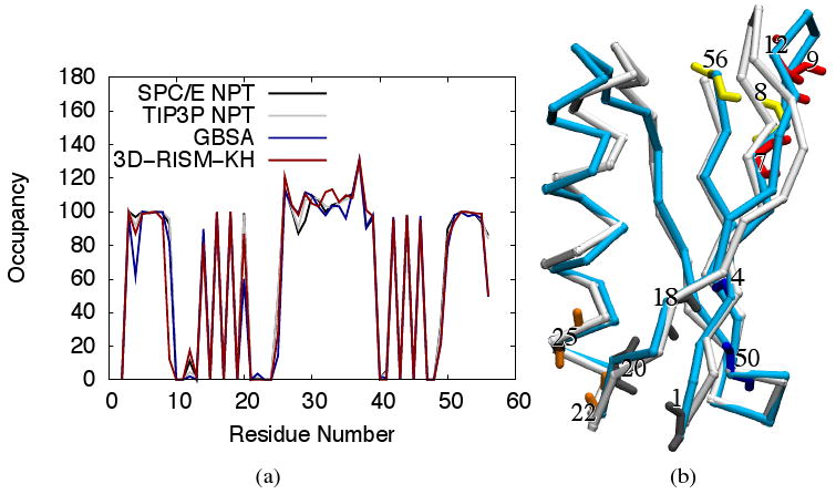
(a) Occupancies for internal backbone hydrogen bonding of protein-G for explicit, implicit and 3D-RISM-KH solvent models. Occupancies >100% indicate bifurcated hydrogen bonds. (b) 3D trace of Cα atoms for NMR structure (PDB ID: 1P7E) in white and final 3D-RISM-KH structure in cyan. Backbone atoms are shown for residues with hydrogen bonding that differs from explicit solvent simulation. Images are made with VMD.71,72
Hydrogen bonding between residues LYS4 and LYS50 is primarily an issue for GBSA. As this is at the end of a β-sheet, it may indicate some additional flexibility, even unzipping, of the sheet. If the hydrogen bond cut-off criteria is extended to 4.0 Å from 3.5 Å, the occupancy exceeds 80%. Enhanced flexibility also appears to be the cause for reduced hydrogen bonding between THR25 (NH) and ASP22 (CO) for non-explicit models with 14% and 28% occupancy for GBSA and 3D-RISM-KH compared to 40% and 50% for SPC/E and TIP3P.
The loop consisting of residues 9 through 12 is a site of qualitative difference in structure (Figure 12(b)) and behavior (Figure 13) of the 3D-RISM-KH simulation from other solvation models. While a stable hydrogen bond is seen for GBSA (81%), SPC/E (80%) and TIP3P (94%) 3D-RISM-KH shows an occupancy of only 12% for a GLY9 (NH) to LEU12 (CO). In contrast, 3D-RISM-KH also shows an occupancy of 17% for a LEU12 (NH) to GLY9 (CO) while the three other methods only show a 1-2% occupancy. This suggests that there is a oscillation between two weak hydrogen bonds. Indeed, in Figure 13(b) and (c) the GLY9 (NH) to LEU12 (CO) hydrogen bond is disrupted by solvent. The overall effect is to bend this loop out from the protein core into the solvent (12b).
Figure 13.
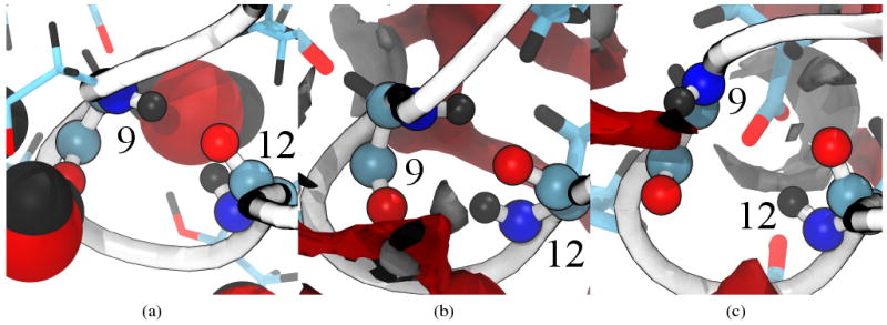
Backbone hydrogen bonding between residues 9 and 12 for representative structures of (a) explicit SPC/E, (b) 3D-RISM-KH with hydrogen bonding and (c) 3D-RISM-KH without hydrogen bonding. Protein backbone drawn as a white tube, backbone atoms for residues 9 and 12 as spheres and side chains as sticks. Carbons are cyan, oxygens red, hydrogens black and nitrogens blue. Solvent density isosurfaces are shown at for both oxygen (red) and hydrogen (gray). Images made with VMD.71,72
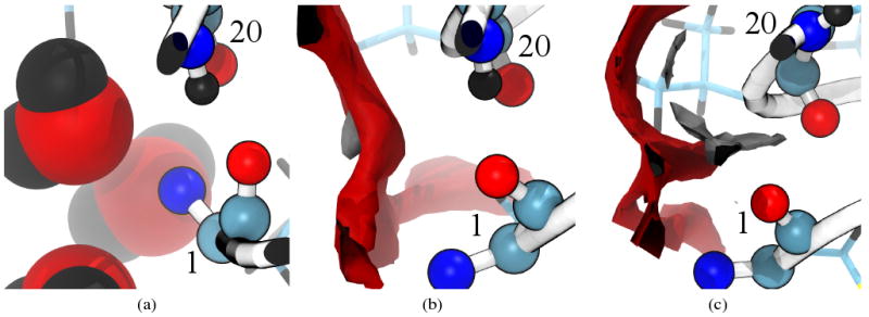
Residue ALA20 is another site where it would appear that GBSA has failed to capture the correct hydrogen bonding; however, the situation is somewhat more complex. The ALA20 (NH) site is 60% occupied in hydrogen bonding but this bonding is strictly with THR18 (CO). For SPC/E and TIP3P ALA20 (NH) has no hydrogen bonding with THR18 but 99% and 100% respectively with MET1. 3D-RISM-KH, however, has ALA20 (NH) binding to both THR18 and MET1, 54% and 33% respectively. The correct behavior in this case is not clear. Clore and Gronenborn,73 on the basis of nuclear magnetic resonance (NMR) data, proposed a three site bifurcated hydrogen bond between ALA20 (NH), MET1 (CO) and a bound water molecule with residence time > 1 ns. In an explicit solvent MD simulation Sheinerman and Brooks68 observed a long residence time water in this location but, in this case, there was no direct hydrogen bond between ALA20 (NH) and MET1 (CO) and the water served as an intermediary between the two residues. No such long residence time water is observed in our explicit solvent simulations, though the residues are highly solvated (Figure 14(a)). For our 3D-RISM-KH simulation, however, the hydrogen bond is broken by the solvent (Figure 14(c)), re-formed (Figure 14(b)) and broken again in the course of the 600 ps simulation.
Figure 14.
Backbone hydrogen bonding between residues 1 and 20 for representative structures of (a) explicit SPC/E, (b) 3D-RISM-KH with hydrogen bonding and (c) 3D-RISM-KH without hydrogen bonding. Coloring as in Figure 13. Images made with VMD.71,72
As well, Clore and Gronenborn also proposed that a similar long residence time water would stabilize a hydrogen bond between TYR33 (NH) and ALA29 (CO). Neither the explicit simulations nor the 3D-RISM-KH simulation showed any water situated to do this, though the site was well hydrated. This is in agreement with the observations of Sheinerman and Brooks.
Both GBSA and 3D-RISM-KH have 50% occupancy for the hydrogen bond between GLU56 (NH) and ASN8 (CO) compared to 75% and 79% for SPC/E and TIP3P. However, the reason for the low occupancy for 3D-RISM-KH is due to a larger systematic problem. As shown in Figure 15, a large, solvated cleft opens into the hydrophobic interior of the protein in the 3D-RISM-KH simulation. This allows the GLU56 (NH) and ASN8 (CO) pair to be solvated such that the hydrogen bond is disrupted. As pointed out by Kovalenko and Hirata,48 this is likely due to the overestimation of solvent ordering around the hydrophobic sidechains at the core of the protein. This is a shortcoming of the KH closure, though the same deficiency was originally identified in the HNC closure equation. As such, it is not a shortcoming of 3D-RISM and can be overcome with an improved closure, though sure a development is not a trivial task.
Figure 15.
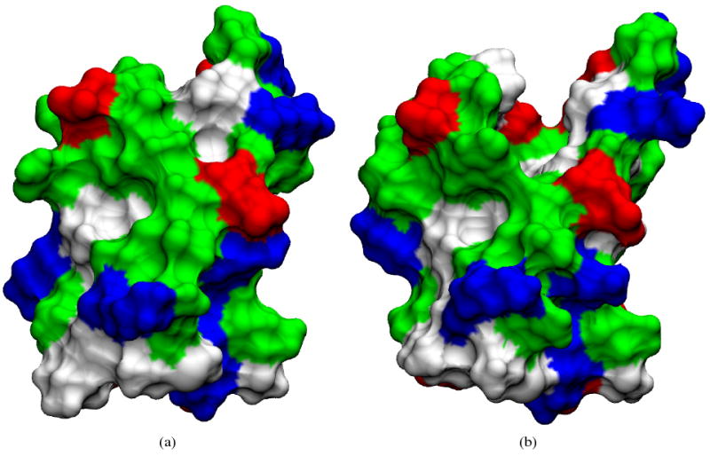
Solvent accessible surface area for protein G simulated with (a) explicit SPC/E and (b) 3D-RISM-KH. Surface is colored by residue type: acid (red), base (blue), polar (green) and non-polar (white). Images made with VMD71,72,74
5 Conclusions
We have presented an efficient coupling of molecular dynamics simulation with the three-dimensional molecular theory of solvation (3D-RISM-KH), contracting the solvent degrees of freedom, and have implemented this multiscale method in the Amber molecular dynamics package.
The 3D-RISM-KH theory uses the first principles of statistical mechanics to provide proper account of molecular specificity of both the solute biomolecule and solvent. This includes such effects as hydrogen bonding both between solvent molecules and between the solute and solvent, hydrophobic hydration and hydrophobic interaction. The 3D-RISM-KH theory readily addresses electrolyte solutions and mixtures of liquids of given composition and thermodynamic conditions. As the solvation theory works in a full statistical-mechanical ensemble, the coupled method yields solvent distributions without statistical noise, and further, gives access to slow processes like hydration of inner spaces and pockets of biomolecules.
The use of 3D-RISM, a mean-field method contracting the solvent degrees of freedom in a statistical-mechanical average means that the solvent dynamics are lost and the observed trajectories in any case are not true dynamics of MD simulation with explicit solvent. They are driven largely by a solvent-mediated potential of mean force, that is, by the probability of finding the biomolecule in a particular conformation, sampled over an ensemble of solvation shell arrangements which frequently require extremely long time to get realized (e.g. opening of protein parts to let solvent molecules or ions in to the inner spaces or pockets, multiply repeated to reach proper statistics). However, such trajectories in a solvent potential of mean force preserve the thermodynamic properties such as conformational distribution of the biomolecule and efficiently sample the conformational space regions of interest in a number of molecular biology problems such as functioning of biomolecular structures (e.g. biological channels and chaperons), protein folding, aggregation, and ligand binding.
Arrangements of solution species in the solvation shells of the biomolecule, sampled by the 3D-RISM-KH theory can include structural solvent and/or cosolvent molecules and other associating structures like salt bridges, buffer ions, and associated ligand molecules. In the latter case, ligand molecules (or their relatively small fragments) at a given concentration in solution are described as a component of solvent at the level of site-site RISM theory and then mapped onto the biomolecule surface by the 3D-RISM method identifying the most probable binding modes of ligand molecules.24 Together with MD sampling of biomolecular conformations, this opens up a new computational method for fragment-based drug design which provides proper, statistical-mechanical account of solvation forces with self-consistent coupling of both non-polar and polar components and which gives access to binding events accompanied with rearrangements of the biomolecule and solvent on a long-time scale.
The implementation includes several procedures to maximally speed up the calculation: (i) cut-off procedures for the Lennard-Jones and electrostatic potentials and the forces acting on the solute, (ii) cut-offs and approximations for the asymptotics of the 3D site correlation functions of solvent, (iii) an iterative guess for the solution to the 3D-RISM-KH equations by extrapolating the past solutions, (iv) multiple time step (MTS) interpolation of solvation forces between the successive 3D-RISM-KH evaluations of the forces, which are then extrapolated forward at the MD steps until the next 3D-RISM evaluation.
As a preliminary validation, we have applied the method to alanine-dipeptide and protein G in ambient water. Analysis of the accuracy of forces, energy and temperature, including such known artifacts as net force drift, has been performed; factors affecting the accuracy have been quantified and the range of grid resolution and tolerance parameters ensuring reliable results has been outlined. The performance of the coupled method has been characterized, compared to MD with explicit and implicit solvent. This work is a preliminary but significant step toward the full-scale characterization and analysis of the new method, and further improvement of its performance to address slow processes of large biomolecules in solution.
Acknowledgments
This work was supported by the Natural Sciences and Engineering Research Council (NSERC) of Canada and the National Research Council (NRC) of Canada. All calculations were performed on the HPC cluster of the Center of Excellence in Integrated Nanotools (CEIN) at the University of Alberta. T.L. acknowledges financial support from NSERC, NRC, and the University of Alberta.
References
- 1.Case D, Cheatham T, Darden T, Gohlke H, Luo R, Merz K, Onufriev A, Simmerling C, Wang B, Woods R. J Comput Chem. 2005;26:1668–1688. doi: 10.1002/jcc.20290. [DOI] [PMC free article] [PubMed] [Google Scholar]
- 2.Still W, Tempczyk A, Hawley R, Hendrickson T. J Am Chem Soc. 1990;112:6127–6129. [Google Scholar]
- 3.Chandler D, McCoy J, Singer S. J Chem Phys. 1986;85:5971–5976. [Google Scholar]
- 4.Chandler D, McCoy J, Singer S. J Chem Phys. 1986;85:5977–5982. [Google Scholar]
- 5.Beglov D, Roux B. J Phys Chem B. 1997;101:7821–7826. [Google Scholar]
- 6.Kovalenko A, Hirata F. Chem Phys Lett. 1998;290:237–244. [Google Scholar]
- 7.Kovalenko A, Hirata F. J Chem Phys. 1999;110:10095–10112. [Google Scholar]
- 8.Kovalenko A, Hirata F. J Chem Phys. 2000;112:10391–10402. [Google Scholar]
- 9.Kovalenko A, Hirata F. J Chem Phys. 2000;112:10403–10417. [Google Scholar]
- 10.Kovalenko A. In: Molecular Theory of Solvation. Chapter 4. Hirata F, editor. Vol. 24. Kluwer Academic Publishers; Norwell, MA, USA: 2003. pp. 169–276. [Google Scholar]
- 11.Hansen JP, McDonald I. Theory of Simple Liquids. 3rd ed. Elsevier; Amsterdam, the Netherlands: 2006. [Google Scholar]
- 12.Beglov D, Roux B. J Chem Phys. 1995;103:360–364. [Google Scholar]
- 13.Yoshida K, Yamaguchi T, Kovalenko A, Hirata F. J Phys Chem B. 2002;106:5042–5049. [Google Scholar]
- 14.Omelyan I, Kovalenko A, Hirata F. J Theor Comput Chem. 2003;2:193–203. [Google Scholar]
- 15.Gusarov S, Ziegler T, Kovalenko A. J Phys Chem A. 2006;110:6083–6090. doi: 10.1021/jp054344t. [DOI] [PubMed] [Google Scholar]
- 16.Casanova D, Gusarov S, Kovalenko A, Ziegler T. J Chem Theory Comput. 2007;3:458–476. doi: 10.1021/ct6001785. [DOI] [PubMed] [Google Scholar]
- 17.Moralez J, Raez J, Yamazaki T, Motkuri R, Kovalenko A, Fenniri H. J Am Chem Soc Communications. 2005;127:8307–8309. doi: 10.1021/ja051496t. [DOI] [PubMed] [Google Scholar]
- 18.Johnson R, Yamazaki T, Kovalenko A, Fenniri H. J Am Chem Soc. 2007;129:5735–5743. doi: 10.1021/ja0706192. [DOI] [PubMed] [Google Scholar]
- 19.Tikhomirov G, Yamazaki T, Kovalenko A, Fenniri H. Langmuir. 2008;24:4447–4450. doi: 10.1021/la8001114. [DOI] [PubMed] [Google Scholar]
- 20.Yamazaki T, Fenniri H, Kovalenko A. Chem Phys Chem. 2010 doi: 10.1002/cphc.200900324. accepted. [DOI] [PubMed] [Google Scholar]
- 21.Drabik P, Gusarov S, Kovalenko A. Biophys J. 2007;92:394–403. doi: 10.1529/biophysj.106.089987. [DOI] [PMC free article] [PubMed] [Google Scholar]
- 22.Yamazaki T, Imai T, Hirata F, Kovalenko A. J Phys Chem B. 2007;111:1206–1212. doi: 10.1021/jp064615f. [DOI] [PubMed] [Google Scholar]
- 23.Yoshida N, Imai T, Phongphanphanee S, Kovalenko A, Hirata F. J Phys Chem B Feature Article. 2009;113:873–886. doi: 10.1021/jp807068k. and references therein. [DOI] [PubMed] [Google Scholar]
- 24.Imai T, Oda K, Kovalenko A, Hirata F, Kidera A. J Am Chem Soc. 2009;131:12430–12440. doi: 10.1021/ja905029t. [DOI] [PubMed] [Google Scholar]
- 25.Miyata T, Hirata F. J Comput Chem. 2008;29:871–882. doi: 10.1002/jcc.20844. [DOI] [PubMed] [Google Scholar]
- 26.Tuckerman M, Berne B, Martyna G. J Chem Phys. 1991;94:6811–6815. [Google Scholar]
- 27.Tuckerman M, Berne B, Martyna G. J Chem Phys. 1992;97:1990–2001. [Google Scholar]
- 28.Pulay P. Chem Phys Lett. 1980;73:393–398. [Google Scholar]
- 29.Saad Y, Schultz M. J Sci Stat Comput. 1986;7:856–869. [Google Scholar]
- 30.Perkyns J, Pettitt B. J Chem Phys. 1992;97:7656–7666. [Google Scholar]
- 31.Perkyns J, Pettitt B. Chem Phys Lett. 1992;190:626–630. [Google Scholar]
- 32.Burkardt J. [2008/06/12];BLEND: Transfinite Interpolation. http://people.scs.fsu.edu/∼burkardt/f_src/blend/blend.html.
- 33.Allen M, Tildesley D. Computer simulation in chemical physics. Chapter 4. Oxford University Press; Oxford, UK: 1993. pp. 140–181. [Google Scholar]
- 34.Kovalenko A, Hirata F. J Chem Phys. 2000;112:10391–10402. [Google Scholar]
- 35.Barth E, Schlick T. J Chem Phys. 1998;109:1633–1642. [Google Scholar]
- 36.Barash D, Yang L, Qian X, Schlick T. J Comput Chem. 2003;24:77–88. doi: 10.1002/jcc.10196. [DOI] [PubMed] [Google Scholar]
- 37.Schlick T. Molecular modeling and simulation: an interdisciplinary guide. 1st. Springer-Verlag New York, Inc.; Secaucus, NJ, USA: 2002. [Google Scholar]
- 38.Batcho P, Case D, Schlick T. J Chem Phys. 2001;115:4003–4018. [Google Scholar]
- 39.Qian X, Schlick T. J Chem Phys. 2002;116:5971–5983. [Google Scholar]
- 40.Frigo M. SIGPLAN Not. 1999;34:169–180. [Google Scholar]
- 41.Berendsen H, Grigera J, Straatsma T. J Phys Chem. 1987;91:6269–6271. [Google Scholar]
- 42.Jorgensen W, Chandrasekhar J, Madura J, Impey R, Klein M. J Chem Phys. 1983;79:926–935. [Google Scholar]
- 43.Pettitt B, Rossky P. J Chem Phys. 1982;77:1451–1457. [Google Scholar]
- 44.Hirata F, Levy RM. Chem Phys Lett. 1987;136:267–273. [Google Scholar]
- 45.Sato H, Hirata F. J Chem Phys. 1999;111:8545–8555. [Google Scholar]
- 46.Cortis C, Rossky P, Friesner R. J Chem Phys. 1997;107:6400–6414. [Google Scholar]
- 47.Du Q, Beglov D, Roux B. J Phys Chem B. 2000;104:796–805. [Google Scholar]
- 48.Kovalenko A, Hirata F. J Chem Phys. 2000;113:2793–2805. [Google Scholar]
- 49.Dyer K, Perkyns J, Stell G, Pettitt B. J Chem Phys. 2008;129:104512–104520. doi: 10.1063/1.2976580. [DOI] [PMC free article] [PubMed] [Google Scholar]
- 50.Gendre L, Ramirez R, Borgis D. Chem Phys Lett. 2009;474:366–370. [Google Scholar]
- 51.Sumi T, Sekino H. J Chem Phys. 2006;125:034509–034509. doi: 10.1063/1.2390704. [DOI] [PubMed] [Google Scholar]
- 52.Urbic T, Vlachy V, Kalyuzhnyi Y, Dill K. J Chem Phys. 2003;118:5516–5525. [Google Scholar]
- 53.Loncharich R, Brooks B, Pastor R. Biopolymers. 1992;32:523–535. doi: 10.1002/bip.360320508. [DOI] [PubMed] [Google Scholar]
- 54.Ryckaert J, Ciccotti G, Berendsen H. J Comput Phys. 1977;23:327–341. [Google Scholar]
- 55.Mongan J, Simmerling C, McCammon J, Case D, Onufriev A. J Chem Theory Comput. 2007;3:156–169. doi: 10.1021/ct600085e. [DOI] [PMC free article] [PubMed] [Google Scholar]
- 56.Essmann U, Perera L, Berkowitz M, Darden T, Lee H, Pedersen L. J Chem Phys. 1995;103:8577–8593. [Google Scholar]
- 57.Duan Y, Wu C, Chowdhury S, Lee MC, Xiong G, Zhang W, Yang R, Cieplak P, Luo R, Lee T, Caldwell J, Wang J, Kollman P. J Comput Chem. 2003;24:1999–2012. doi: 10.1002/jcc.10349. [DOI] [PubMed] [Google Scholar]
- 58.Simmerling C, Strockbine B, Roitberg A. J Am Chem Soc. 2002;124:11258–11259. doi: 10.1021/ja0273851. [DOI] [PubMed] [Google Scholar]
- 59.Ulmer T, Ramirez B, Delaglio F, Bax A. J Am Chem Soc. 2003;125:9179–9191. doi: 10.1021/ja0350684. [DOI] [PubMed] [Google Scholar]
- 60.Press W, Teukolsky S, Vetterling W, Flannery B. Numerical recipes in FORTRAN: the art of scientific computing. 2nd. Cambridge University Press; New York, NY, USA: 1992. [Google Scholar]
- 61.Roe D, Okur A, Wickstrom L, Hornak V, Simmerling C. J Phys Chem B. 2007;111:1846–1857. doi: 10.1021/jp066831u. [DOI] [PMC free article] [PubMed] [Google Scholar]
- 62.Soper A, Phillips M. Chem Phys. 1986;107:47–60. [Google Scholar]
- 63.Still W, Tempczyk A, Hawley R, Hendrickson T. J Am Chem Soc. 1990;112:6127–6129. [Google Scholar]
- 64.Levy R, Zhang L, Gallicchio E, Felts A. J Am Chem Soc. 2003;125:9523–9530. doi: 10.1021/ja029833a. [DOI] [PubMed] [Google Scholar]
- 65.Gonçalves P, Stassen H. Pure Appl Chem. 2004;76:231UŰ–240. [Google Scholar]
- 66.Liu P, Kim B, Friesner R, Berne B. Proc Natl Acad Sci USA. 2005;102:13749–13754. doi: 10.1073/pnas.0506346102. [DOI] [PMC free article] [PubMed] [Google Scholar]
- 67.Kwac K, Lee KK, Han JB, Oh KI, Cho M. J Chem Phys. 2008;128:105106. doi: 10.1063/1.2837461. [DOI] [PubMed] [Google Scholar]
- 68.Sheinerman F, C B., III Proteins: Struct Func Genet. 1997;29:193–202. doi: 10.1002/(sici)1097-0134(199710)29:2<193::aid-prot7>3.0.co;2-e. [DOI] [PubMed] [Google Scholar]
- 69.Patel S, Jr, A M, C B., III J Comput Chem. 2004;25:1504–1514. doi: 10.1002/jcc.20077. [DOI] [PubMed] [Google Scholar]
- 70.Calimet N, Schaefer M, Simonson T. Proteins: Struct Func Genet. 2001;45:144–158. doi: 10.1002/prot.1134. [DOI] [PubMed] [Google Scholar]
- 71.Humphrey W, Dalke A, Schulten K. Journal of Molecular Graphics. 1996;14:33–38. doi: 10.1016/0263-7855(96)00018-5. [DOI] [PubMed] [Google Scholar]
- 72.Stone J. MSc thesis. Computer Science Department, University of Missouri-Rolla; 1998. [Google Scholar]
- 73.Clore G, Gronenborn A. J Mol Biol. 1992;223:853–856. doi: 10.1016/0022-2836(92)90247-h. [DOI] [PubMed] [Google Scholar]
- 74.Sanner M, Olsen A, Spehner JC. Fast and Robust Computation of Molecular Surfaces. Proceedings of the 11th ACM Symposium on Computational Geometry; New York. 1995. pp. C6–C7. [Google Scholar]