Model Based Unsupervised Learning Guided by Abundant Background Samples

Abstract

Many data sets contain an abundance of background data or samples belonging to classes not currently under consideration. We present a new unsupervised learning method based on Fuzzy C-Means to learn sub models of a class using background samples to guide cluster split and merge operations. The proposed method demonstrates how background samples can be used to guide and improve the clustering process. The proposed method results in more accurate clusters and helps to escape locally minimum solutions. In addition, the number of clusters is determined for the class under consideration. The method demonstrates remarkable performance on both synthetic 2D and real world data from the MNIST dataset of hand written digits.

1. Introduction

Clustering is the process of dividing data samples into groups of similar items. For machine learning, it had been used as a way of discovering and describing hidden models or patterns in a given dataset. Such a process has demonstrated a great ability for learning sub-model parameters and has shown to be very useful in applications of pattern recognition and image segmentation. Recent reviews on clustering algorithms and their applications are available [1], [2].

Fuzzy C-means [3], [4] is one of the most popular and widely used clustering algorithms due to its simplicity, easy convergence, and its scalability to higher dimensions. However, FCM and other clustering algorithms suffer from few drawbacks: 1) the number of clusters must be known a priori and provided by the user; 2) their tendency to fall in local optimal solutions; 3) sensitivity to outliers. Furthermore, the globally optimal solution might not be the best one to describe the hidden models or patterns because the data could be misrepresented, insufficiently distributed or the numerical representations of the features are not descriptive of the true patterns. Many solutions have been already proposed [5]-[8] where most of them begin with a set of initial clusters followed by split, merge or cancelation operations until some acceptable state of clusters is reached. Other methods require user feedback to correct the clustering in a semi-supervised process [9]-[12].

In this paper we propose a new learning method that can be applied to a special case of problems where there is an abundance of background samples or samples that belong to other classes that exist in the same feature space. In many real world applications, we could be confronted with datasets from two classes, foreground and background. For example in the land mine detection problem, there are mine and non-mine images. In bioinformatics, there are promoters and non-promoters and genes and non-genes. One commonality in this category of data sets is that there are always reasons for the differentiation of characteristics between the foreground and the background. For example, in DNA, promoters contain specific motifs or features that make them work as promoters, while non-promoters do not. Therefore, it makes sense to run pattern recognition or clustering processes in the foreground and not in the background. However, background samples may be available in greater quantity than the foreground. Ignoring it in the learning process would waste potentially useful information. However, samples from the background are still likely to be biased. They may be completely random and sparsely populated, and hence are much less informative about the foreground models than the foreground itself.

The proposed method employs an unsupervised learning method: Fuzzy C-Means with fuzzy covariance [4] to learn the hidden patterns of the sub-models of the foreground samples and guide this learning process with knowledge of the background samples. Afterward, the quality of the clusters is evaluated based on how much they overlap with the background. A cluster that overlaps considerably is a good candidate for splitting in a direction to minimize the overlap. Two clusters that are close in the space and whose merge results a new cluster minimally overlapping with the background samples are good candidates for merging. Such a merge and split strategy with appropriate thresholds can provide a useful solution to the aforementioned problems of the FCM and other unsupervised learning methods. A state of the clusters where the overlap between the clusters and the background is minimal is a state that is very likely to contain an appropriate number of clusters of the foreground and less likely to mistakenly take two patterns into one because such model is more likely to overlap with the background and be split.

Even though the training samples are labeled, the method is still an unsupervised learning approach because the goal of the learning is to uncover the sub-patterns or models of the main class and separate them into meaningful groupings. Furthermore, through the proposed method, the boundaries between the main class samples and the rest of the data or the background are enhanced by minimizing the overlap. As a result, such a learning process can be used to build an efficient classifier to discriminate foreground samples from the background or from samples belonging to other classes.

The performance of the proposed technique is demonstrated on both a synthetic 2D moderately complex dataset and a multidimensional dataset from the MNIST hand written digits. In both cases it is shown how advantageous it is to use background samples to guide the learning process. The proposed method performance is compared against the regular FCM algorithm using both datasets and against the hierarchal agglomerative algorithm [13] using the MNIST dataset only. Both algorithms cluster foreground samples without any utilization of background information.

2. Methods

The proposed method iteratively uses the FCM clustering algorithm to refine and estimate clusters by applying split and merge operations in a direction to minimize the overlap between the foreground clusters and the background samples.

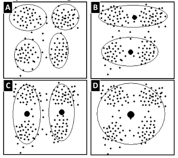
Figures 1 and 2 show a hypothetical data set for the purpose of explanation. In figure 1, samples from the foreground data are being displayed along with different initial candidate solutions (a, b, c or d). If the background samples in the learning process are considered (Figure 2), solution (b) becomes more plausible since it minimizes background overlap, or misclassification, with fewer clusters. Such learning is a competition between background and foreground over the empty space surrounding the foreground models. There is no neutral space, since every spot should either belong to a foreground sub-model or to the background. It is only empty because there are not enough samples to fill all the space. On the other hand, the low number of clusters is favorable because it counters over-fitting. This is why solution (b) might be considered better than solution (a) even if it involved adding slightly more noise.

Figure 1. Alternative clustering solutions for a hypothetical dataset.

Figure 2. Solution (1-B) considering the background information shown in (A).

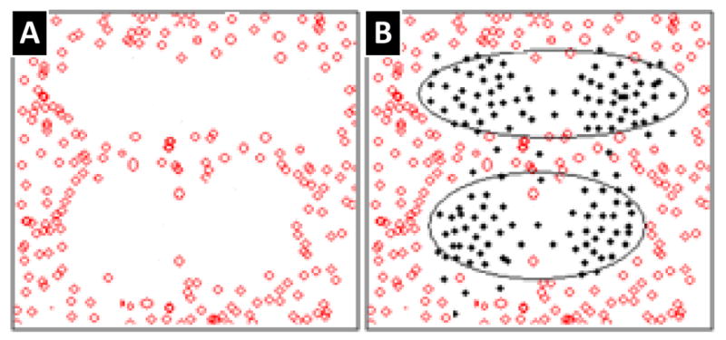
A low level of noise can still be acceptable and expected due to dimension reduction and information loss, bad features or incorrect data. Therefore, the question of when to split or merge is dependent on the dataset and the quantity of the background samples compared to the foreground.

Using the split and merge strategy with appropriate thresholds, if a suboptimal solution (a), (c) or (d) was initially found, solution (b) can still be obtained by the proposed refinement process.

2.1. Fuzzy C-Means with Fuzzy Covariance

Fuzzy c-means (FCM) with fuzzy covariance matrix clustering algorithm was introduced in [4] and is used as the base method for learning the parameters of models. However, other unsupervised learning methods like ML-EM [13], [14] can also be extended to work with the proposed learning refinement method.

FCM is an iterative algorithm that starts with k initial clusters and iteratively re-estimates the parameters of every cluster along with the degree at which every sample belongs to every cluster. This is accomplished by minimizing the objective function given in (1).

$$J=\sum _{i=1}^n\sum _{j=1}^k{u}_{ij}^m{d}_{ij}^2$$ (1)

subject to the constraints:

$$u_{ij}\in [0,1]\forall i,j\text{and}\sum _j^{\text{k}}{u}_{ij}=1,\forall i$$ (2)

In (1), u_ij is the membership of sample i in cluster j and d_ij is the distance between them while m is the fuzziness factor of the algorithm.

With a fuzzy covariance matrix, the distance between sample i with a feature vector of {x_i} and cluster j of mean μ_j and covariance Cj in the case of n dimensions becomes:

$$d_{ij}^2={|C_{\text{j}}|}^{\frac{1}{\text{n}}}{(x_i-{\mu }_j)}^{\text{T}}{C}_j^{-1}(x_i-{\mu }_j)$$ (3)

Due to the limited number of training samples, covariance regularization issues and performance issues [15], all experiments in this paper are restricted to the diagonal covariance matrix case. Also, for all experiments in this paper, covariances are regularized using a simple method described in [16].

$$C_j^{\prime }=\gamma C_j+(1-\gamma )\overline{C}+\in$$ (4)

In (4), C̄ is the average covariance matrix and I is the identity matrix. γ and ε are constant values chosen to be 0.92 and 1^-5 respectively and are designed to prevent extreme bias and zero values along the diagonal respectively. More complex regularization methods have described in [15], [17].

2.2. Cluster adequacy

Every cluster is expected to represent an estimation of a true model in the foreground. Therefore, any cluster should have a distance threshold boundary. Any given sample whose feature vector falls within the boundary is expected to belong to this model and hence belong to the foreground. Anything out of the boundary does not belong to this model. Therefore, for every cluster θ_j, a boundary distance h_j needs to be determined such that the classification error E_j is minimal:

$$\begin{array}{l}\text{E}({\theta }_{\text{j}})={\text{E}}_{\text{j}}\\ =min{arg}_{hj}\left[\sum _{i\in \left\{{\theta }_j\right\}}\phi (d_{ij}>h_j)+\sum _{z\in \left\{\text{bg}\right\}}\phi (d_{zj}\le h_j)\right]\end{array}$$ (5)

Where φ(ν)= $\{\begin{array}{c}1\text{if}\nu =\text{ture}\\ 0\text{if}\nu =\text{false}\end{array}$

And the true classifications become

$$\text{T}({\theta }_j)=T_j=\sum _{i\in \left\{{\theta }_j\right\}}\phi (d_{ij}\le h_j)$$ (6)

In (5) and (6), {θ_j} and {bg} refer to the set of samples from the foreground that belong to cluster j and the set of all background samples respectively.

The ratio of error classifications E_j to the true classifications T_j will be used as a measure of how bad a cluster is.

$$ET{R}_j=\frac{E_j}{T_j+1}$$ (7)

In (7), 1 was added to the denominator in order to avoid division by zero.

2.3. Cluster Split

A cluster that produces a high error ratio in (7) does not provide a good estimate of any true model and is likely to be the result of a local minimum in the learning. Therefore, after every learning phase, the error ratio of every cluster is evaluated and the one with the highest error ratio is split if the error ratio exceeds a threshold S-Threshold.

2.3.1. Split process

Once a cluster θ_j is selected to be split, a random split method may worsen and degrade the learning. However, since performing additional analysis on a single cluster is computationally feasible, cluster θ_j is split along the best dimension ι that results in two clusters $\left\{{\theta }_{\text{j}\iota }^1,{\theta }_{\text{j}\iota }^2\right\}$ with a minimal classification error. It is still preferable to minimize the dispersion of every cluster and hence a split along a dimension where the variance is large is preferred. Therefore, every candidate split $\left\{{\theta }_{\text{j}\iota }^1,{\theta }_{\text{j}\iota }^2\right\}$ along dimension ι is evaluated by:

$$\text{spilt}({\theta }_j,\iota )=\frac{1}{{\sigma }_{j\iota }^{\text{p}}}[\text{E}({\theta }_{j\iota }^1)+\text{E}({\theta }_{j\iota }^2)+1]$$ (8)

In (8) σ_jι is the standard deviation of the cluster θ_j along the dimension ι and p is a scaling factor. A high value of p gives more importance to the split against large variance and dispersion than splits resulting in new clusters away from the background. For experiments in this paper p = 0.5 was used. The second term represents the optimal classification error caused by the new clusters and one is added to prevent the dominance of zero. Therefore, a smaller value in (8) results in a better candidate split. Splits are therefore produced against the dispersion and in away to result in less noisy clusters.

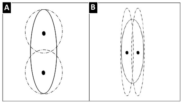
As a rough approximation for the clusters resulting from splitting cluster θ_j along dimension ι, the samples in cluster θ_j are split by the hyper plane passing through the center of θ_j and orthogonal to the axis ι. Afterward, the two resulting sets of samples are used to estimate the parameters of the new clusters: $\left\{{\theta }_{\text{j}\iota }^1,{\theta }_{\text{j}\iota }^2\right\}$. Figure 3 shows two schematic different candidate splits.

Figure 3. Initial candidate splits along (a) the vertical and (b) horizontal axes.

2.4. Merging two clusters

Merging clusters has been used heavily in hierarchal agglomerative clustering [1], [2] where close clusters are merged. In the proposed method, close clusters whose merge will result in minimal overlap with the background samples are favored for merge operations. Two close clusters in the space that have background samples in between are unlikely to belong to one model and are not good candidate for merge.

Ward's linkage method is used to calculate a distance measure or linkage between clusters. This method is based on the analysis of variance (ANOVA) to minimize the sum of variances within clusters. The distance between two clusters {θ_g, θ_j} is computed as the increase in the error sum of squares (ESS) caused by the merge.

$$\text{d}({\theta }_g,{\theta }_j)=\text{ESS}({\theta }_g,{\theta }_j)-\text{ESS}({\theta }_g)-\text{ESS}({\theta }_j)$$ (9)

Where

$$\text{ESS}({\theta }_j)=\sum _{x_i\in \left\{{\theta }_j\right\}}{(x_i-{\mu }_{\text{j}})}^2$$ (10)

Using the distance in (9) a limited set of N pairs with the smallest distances are selected. The distances for all N pairs are normalized by:

$$\text{D}({\theta }_g,{\theta }_j)=D_{g,j}=\frac{\mathit{\text{d}}({\theta }_g,{\theta }_j)}{\mu +2\sigma }$$ (11)

Where μ and σ are the mean and the standard deviation of the distances of the N cluster pairs respectively. The normalization in (11) guarantees that most of the distances will fall in the range [0, 1]. The experiments in this paper set N to be 2k, where k is the number of clusters.

The normalized distance and the resulting error ratio of the merge are used to measure the cost of the merge as:

$$\begin{array}{l}\text{Merge}({\theta }_g,{\theta }_j)=\alpha D_{g,j}\text{MThreshold}\\ +\left(1-\alpha \right)ET{R}_{g,j}\end{array}$$ (12)

In (12) α is a scaling factor whose value is in the range [0, 1]. A value of α close to one results a merge that is only based on the least distance while α close to zero results in a merge based on the least resulting error ratio. For the experiments in this paper, α = 0.4.

The first term in (12) results in an addition of a value in the range of [0, αMThreshold] depending on the relative distance between the clusters pairs. In other words, the merge is penalized depending on the distance to a maximum of αMThreshold, which is a fraction of the merge threshold itself.

The cluster pair with the least merge cost from (12) is anticipated to contain two spatially close clusters. In addition, a merge of this pair is expected to represent a good model estimation that does not overlap with the background. However, the merge cost of the best candidate has to be lower than a threshold (MThreshold).

The complete algorithm is summarized below

• - Initialize the number of clusters, k.

• - Initialize merge and split thresholds {MThreshold, SThreshold}.

• - Initialize cluster centers.

Repeat:

• - Perform FCM to estimate clusters parameters {μ},{θ}.

• - Select the best split cluster as stated in section 2.3.

  • - Perform a split if the error ratio given by (7) is greater than the split threshold.

• - Select best merge pair clusters as stated in section 2.4.

  • - Perform merge if the merge cost given by (12) is less than the merge threshold.

• - Use the new set of clusters to initialize FCM.

Until no more splits or merges were performed.

3. Data Sets

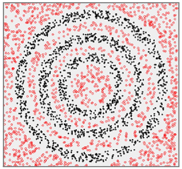
The proposed learning process is tested on two different data sets. The first is a synthetic 2D data set composed of samples from two classes (background and foreground). As shown in figure 4, the foreground samples make up patterns of three circles while the background is everything outside of those patterns.

Figure 4. Synthetic data of two classes. The foreground is represented as solid points and the background consists of hollow points.

The second data set consists of hand written digits extracted from the MNIST database of handwritten digits [18]. 1000 image samples were extracted for every digit {0, 1 … 9}. The digit number 5 was used as the foreground digit of interest and the remaining digits were considered as the abundant background samples.

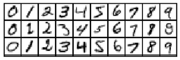
The hand written digits from MNIST are available as images of 28*28 resolution. For the purpose of this research, digits were down sampled into 14*14 by averaging every four pixels as a method for dimension reduction to reduce computation cost. Figure 5 shows sample digits before dimension reduction while figure 6 shows the same images after dimension reduction.

Figure 5. Hand written digits with 28*28 resolution.

Figure 6. 14*14 digits after down sampling by averaging.

4. Results

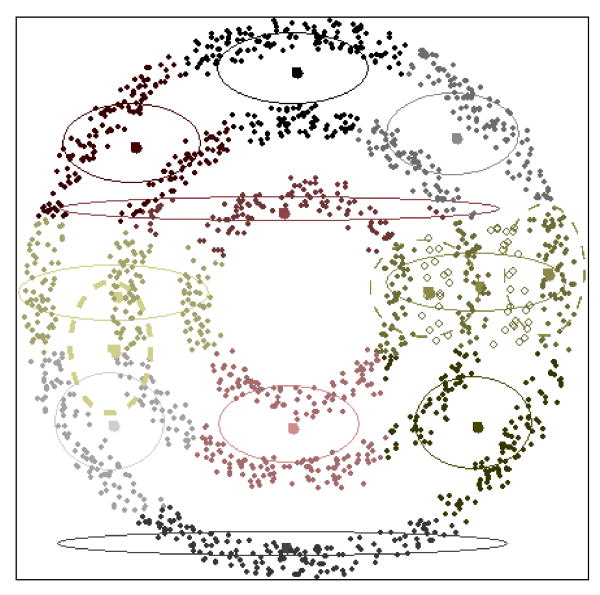
For the first experiment, the synthetic foreground samples were separated into 10 initial clusters in an effort to find representative sub-patterns. Figure 7 shows the initial clusters in solid lines. Models that grasp samples from different concentric rings are not representative of the known solution. In addition, Figure 7 shows the best merge and split candidate clusters. When an error ratio of 0.44 was used for the split threshold (SThreshold) along with a merge threshold (MThreshold) of 0.2, the given split was performed but the candidate merge was ignored.

Figure 7. Initial clusters for synthetic 2D data. The best candidate split shown in a thin dashed line was accepted. The best candidate merge shown as a thick dashed line was rejected. The hollow points indicate noise in the cluster to be split.

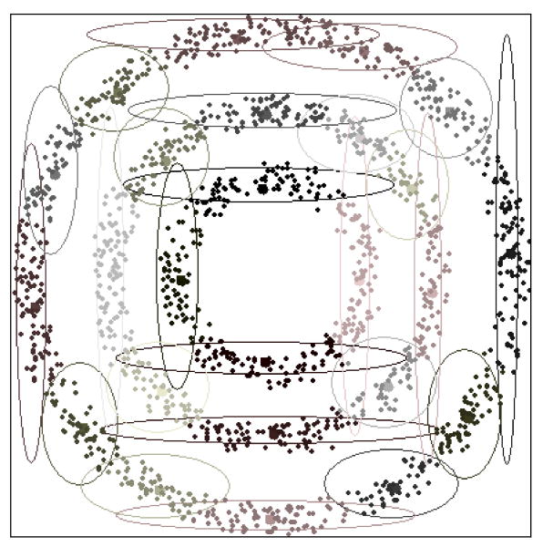
Figure 8 shows the resulting clusters after 20 iterations in which 18 splits and three merges were performed. The result is a set of 25 clusters representing adjacent models on each of the concentric circles.

Figure 8. Optimal results of FCM with split and merge at 25 clusters.

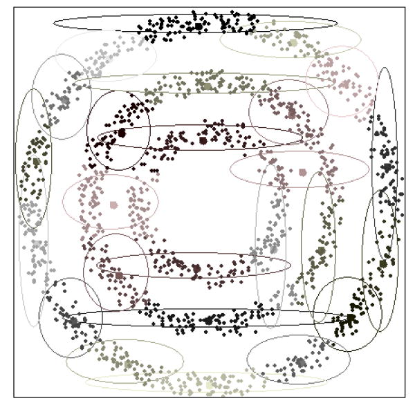
The learning not only leads to an optimal number of clusters, but also alleviates locally optimal solutions. For comparison, clustering using FCM with 25 initial clusters was performed without the proposed merge and split refinement method. What results is a worse set of clusters (Figure 9) where a number of the clusters combine samples from different concentric circles.

Figure 9. FCM clustering into 25 clusters without incorporation of split and merge operations.

For the second experiment, the goal is to learn the sub-models of the handwritten digit 5. Class 5 (consisting of the handwritten digit 5) was used as the foreground and the remaining digits (0-4, 6-9) were considered as the background.

An initial clustering of 45 clusters was performed along with iterative split and merge with a merge threshold of (0.05) and a split threshold of (0.12). Figure 10 shows the number of clusters for each iteration while figure 11 shows the classification error at each iteration.

Figure 10. Number of clusters at every iteration for the handwritten dataset.

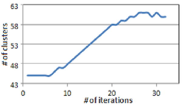
Figure 11. Classification error in every iteration for the handwritten dataset.

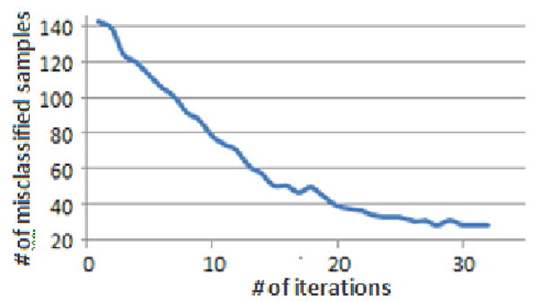
Figure 10 and 11 together provide good decision tool to decide where the learning refinement reaches an acceptable solution. It is apparent that the proposed refinement method decreases the classification error. For example at iteration 6, the number of classification errors drop (141 to 106) without increasing the number of clusters due to simultaneous split and merge operations. On the other hand, at iteration 32, the algorithm converged with 60 clusters where there were no more split or merge candidates within the thresholds. With the resulting 60 clusters the number of misclassified digits dropped from 141 to 29.

The classification error increase for some iterations is expected since the merge and split are not guaranteed to lead to a better clustering. However, whenever it worsens, you would expect more merges and splits to correct the errors.

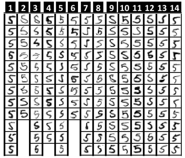
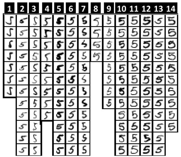
Figure 12 shows some sample subsets of clusters from the initial clustering. If you look into these clusters you will find many images that are not related within the same group. For example, images 2, 3, 8 and 10 in cluster 7 do not look like anything else in the same group. Also the images 4, 5 and 6 in cluster 5 do not look like anything else in the same cluster. Furthermore, images in cluster 2, 3, 8, 9 and 14 have high variation. On the other hand, figure 14 shows clusters from iteration 32. Cluster 1 managed to isolate and group very similar images that were considered before as unrelated in the initial clustering in both clusters 5 and 7. Also if you look in images inside every cluster you will find more homogeneity than in the initial clustering.

Figure 12. Sample clusters from the initial 45 clusters.

To test if the proposed method was able to alleviate bad local minimums and not just to learn the number of clusters, the FCM clustering algorithm was run with a random initial number of clusters. Every clustering size was run five times to compute the average classification error given the number of clusters. Also we compared results to the hierarchal agglomerative clustering that uses FCM with fuzzy covariance to estimate clusters' parameters. The hierarchal agglomerative clustering was initialized to 150 clusters. Wards distance was used to find the closest pair of clusters for merging.

Table I shows the classification errors resulting from each algorithm. As this table indicates, there is considerable learning gain from the proposed split and merge method over both: the flat FCM approach and the hierarchal agglomerative clustering.

Table I. Comparison of Classification Errors.

	Classification Error
Number of clusters	FCM	Hierarchal Agglomerative	Proposed method
45	149	131	106
50	132	101	71
55	105	95	47
60	97	81	29

5. Conclusion

The proposed split and merge method demonstrates an enhanced ability to learn sub models in a feature space rife with background samples. Background information can be used efficiently to guide the learning process. On the other hand, any bias in the available background samples would not worsen the learning since they are not used in estimating the parameters of every model.

The improved learning in the handwritten digits problem is due to the isolation of outliers and unrelated patterns by the split process. In addition, the merge groups similar patterns which in turn provides more samples for a better estimation of a model's true parameters, thus countering the over-fitting effect.

The proposed split and merge method reduces the solution to finding an appropriate number of clusters and avoiding non-descriptive local minimums by specifying split and merge thresholds. These thresholds are intuitive values that can be estimated by comparing the error classification ratio of every model. Appropriate thresholds can be determined by considering initial error rates given by clusters, examining the quality of the data, and evaluating the ratio of the number of background to foreground samples.

The proposed learning method can be of direct use in building classifiers like radial basis function networks, k-nearest neighbors and fuzzy k-neighbors classifiers since it minimizes the overlap between the learnt sub-models of the foreground and background classes, hence providing a more discriminative boundary between them.

Figure 13. Sample clusters from iteration 29.

References

- 1.Xu R, Wunsch D. Survey of clustering algorithms. 2005 May;16(3):645–678. doi: 10.1109/TNN.2005.845141. [DOI] [PubMed] [Google Scholar]
- 2.Berkhin P. Survey Of Clustering Data Mining Techniques. 2002 [Google Scholar]
- 3.Zadeh LA. Fuzzy Sets. Information and Control. 1965;8:332–353. [Google Scholar]
- 4.Gustafson DE, Kessel WC. Fuzzy clustering with a fuzzy covariance matrix. Decision and Control including the 17th Symposium on Adaptive Processes; San Diego, CA. 1978. [Google Scholar]
- 5.Frigui H, Krishnapuram R. Clustering by competitive agglomeration. Pattern Recognition. 1997 Jul;30:1109–1119. [Google Scholar]
- 6.Ueda N, Nakano R, Ghahramani Z, Hinton GE. SMEM algorithm for mixture models. Neural Computation. 2000 Sep;12:2109–2128. doi: 10.1162/089976600300015088. [DOI] [PubMed] [Google Scholar]
- 7.Richardson S, Green PJ. On Bayesian analysis of mixtures with an unknown number of components. Journal of the Royal Statistical Society Series B-Methodological. 1997;59:731–758. [Google Scholar]
- 8.Ball GH, Hall DJ. A clustering technique for summarizing multivariate data. Behavioral Science. 1967;12:153–155. doi: 10.1002/bs.3830120210. [DOI] [PubMed] [Google Scholar]
- 9.B A, M RJ, Basu S. semi-supervised clustering by seeding. Proceedings of the 19th International Conference on Machine Learning; 2002. pp. 19–26. [Google Scholar]
- 10.Basu S, Bilenko M, Mooney RJ. A Probabilistic Framework for Semi-Supervised Clustering. Knowledge Discovery and Data Mining (KDD-2004), 10th ACM SIGKDD Intl; Seattle, WA. 2004. [Google Scholar]
- 11.Zhu X. Semi-supervised learning literature survey. 2005:1530. [Google Scholar]
- 12.Frigui H, Mahdi R. Semi-Supervised Clustering and Feature Discrimination with Instance-Level Constraints. FUZZ-IEEE 2007. IEEE International; 2007. [Google Scholar]
- 13.Dempster AP, Laird NM, Rubin DB. Maximum Likelihood from Incomplete Data Via Em Algorithm. Journal of the Royal Statistical Society Series B-Methodological. 1977;39 [Google Scholar]
- 14.McLachlan G, Krishnan T. The EM Algorithm and Extensions. New York: Wiley; 1997. [Google Scholar]
- 15.Friedman JH. Regularized Discriminant Analysis. Journal of the American Statistical Association. 1989 Mar;84:165–175. [Google Scholar]
- 16.Li J. Regularized Discriminant Analysis and Reduced-Rank LDA. [Online]. http://www.stat.psu.edu/∼jiali/course/stat597e/notes2/lda2.pdf.
- 17.Hoffbeck JP, Landgrebe DA. Covariance Matrix Estimation and Classification with Limited Training Data. IEEE Transactions on Pattern Analysis and Machine Intelligence. 1996 Jul;18(7):763–767. [Google Scholar]
- 18.LeCun Y. The MNIST database of handwritten digits. [Online]. http://yann.lecun.com/exdb/mnist.
- 19.Hartigan JA, Wong MA. A k-means clustering algorithm. 1979 [Google Scholar]
- 20.Hartigan J. Clustering Algorithms. New York, NY: John Wiley & Sons; 1975. [Google Scholar]
- 21.Figueiredo MAT, Jain AK. Unsupervised learning of finite mixture models. IEEE Transactions on Pattern Analysis and Machine Intelligence. 2002 Mar;24:361–396. [Google Scholar]
- 22.Celeux G, Govaert G. A Classification Em Algorithm for Clustering and 2 Stochastic Versions. Computational Statistics & Data Analysis. 1992 Oct;14:315–33. [Google Scholar]
- 23.Duda RO, Hart PE, Stork DG. Pattern Classification. 2nd. 2000. [Google Scholar]