Abstract
Polymer fluids are modeled with dissipative particle dynamics (DPD) as undiluted bead-spring chains and their solutions. The models are assessed by investigating their steady shear-rate properties. Non-Newtonian viscosity and normal stress coefficients, for shear rates from the lower to the upper Newtonian regimes, are calculated from both plane Couette and plane Poiseuille flows. The latter is realized as reverse Poiseuille flow (RPF) generated from two Poiseuille flows driven by uniform body forces in opposite directions along two-halves of a computational domain. Periodic boundary conditions ensure the RPF wall velocity to be zero without density fluctuations. In overlapping shear-rate regimes the RPF properties are confirmed to be in good agreement with those calculated from plane Couette flow with Lees–Edwards periodic boundary conditions (LECs), the standard virtual rheometer for steady shear-rate properties. The concentration and the temperature dependence of the properties of the model fluids are shown to satisfy the principles of concentration and temperature superposition commonly employed in the empirical correlation of real polymer-fluid properties. The thermodynamic validity of the equation of state is found to be a crucial factor for the achievement of time-temperature superposition. With these models, RPF is demonstrated to be an accurate and convenient virtual rheometer for the acquisition of steady shear-rate rheological properties. It complements, confirms, and extends the results obtained with the standard LEC configuration, and it can be used with the output from other particle-based methods, including molecular dynamics, Brownian dynamics, smooth particle hydrodynamics, and the lattice Boltzmann method.
INTRODUCTION
Particle models of complex fluids create the need for methods to calculate the simulated equivalents of the physical properties commonly measured in rheometers. The simulated and measured properties can then be matched to calibrate the model’s parameters. This operation is of great importance, especially in mesoscopic simulations, which attempt to capture the observable properties of complex fluids with coarse graining in space and time. Thus, known atomistic interactions are replaced with soft-type interactions among coarse entities each of which may contain a large number of atoms or molecules. The validity of such models is determined by examination of their macroscopic properties. For models of Newtonian fluids, various methods have been employed for the calculation of viscosity and other transport coefficients. These methods often employ the Green–Kubo (GK) relations derived from correlations of fluctuations about states of equilibrium. In principle, GK theory will deliver only the linear viscoelastic properties of complex fluids. However, steady shear flows at rates beyond the lower Newtonian regime are not states near equilibrium and do not appear to be amenable to the GK analysis. Hence, the virtual analogs of the shear flows of rheometry must be employed to determine the rheology of the simulated complex fluids.
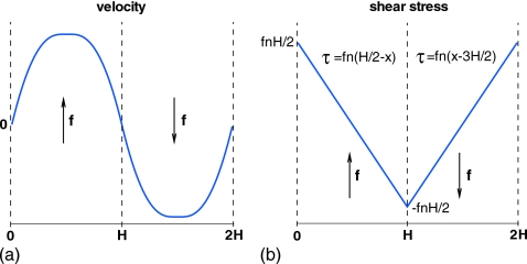
As with experimental rheometry, the response of a test fluid to more than one deformation field is needed for its complete rheological characterization. However, the first step, the subject of this work, is nearly always the response to steady shear flow. Here we investigate the use of reverse Poiseuille flow (RPF) as an alternative virtual rheometer for the calculation of the material functions of steady-state shearing. The application of RPF to complex fluids is novel, although it was first applied to measure the viscosity for particle models of Newtonian fluids.1 The flow consists of two parallel Poiseuille flows driven by uniform body forces of equal magnitude but in opposite directions. Figure 1 shows the profiles of the imposed shear stress (b) and of the resulting velocity (a). Periodic boundary conditions imply that the profiles in Fig. 1 are repeated in each horizontal direction, and hence, they are effectively stationary, spatial waves. The shear rate spans the range from zero along the channel centerline to the maximum wall value. In principle, this means that a single simulation yields the material functions of steady shear over that range of shear rates.
Figure 1.
Typical RPF velocity profile (a) driven by the imposed wall shear stress fnH∕2 (b), where f is the body force per unit mass and n is the number density.
The standard virtual rheometer, widely used in particle simulations to obtain steady-state shear properties, is plane Couette flow with the Lees–Edwards periodic boundary conditions (LECs).2 This configuration has been favored because its shear rate is uniform and prescribed. It is counterintuitive to expect that RPF can yield comparable results with its nonuniform shear rates to be obtained by numerical differentiation. In part, the success of the RPF rheometer is due to the smoothness of the computed velocity profiles, which are averages of the four half-channel profiles, the statistical equivalent to an ensemble average over four replicas in addition to the usual time-averaging over many steps. A less obvious factor may be the benefit of each particle being driven by the same body force in contrast to the wall-driven Couette flow. The periodic boundary conditions of both RPF and LEC eliminate the need for explicit modeling of solid wall boundary conditions. This has the significant advantage of excluding unknown wall effects, such as slip and density fluctuations, which seem to be endemic to particle-wall models as they are currently known. This is of particular importance for fluid mixtures and solutions which exhibit nonuniform concentration profiles as a consequence of cross-stream migration induced by stress gradients.
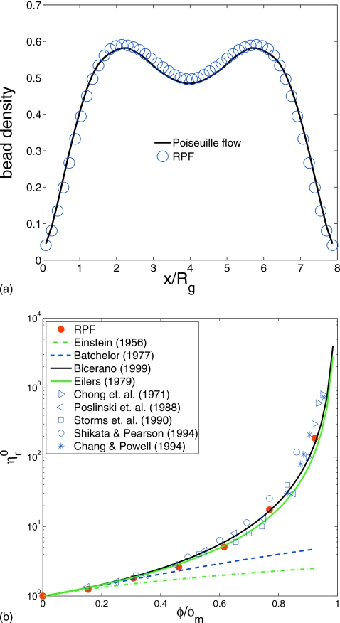
RPF has been applied successfully to dissipative particle dynamics (DPD) simulations of dilute polymer solutions3 and colloidal suspensions.4 Figure 2a shows the bead density profiles of a dilute polymer solution obtained in wall-bounded plane Poiseuille flow and RPF, where Rg is the bead-chain radius of gyration. The agreement shows that the real channel wall, explicitly constructed from fixed DPD-particle layers, behaves similar to the RPF “wall,” a shear plane of zero velocity by virtue of the periodic boundary conditions. Figure 2b demonstrates excellent agreement between the calculated and the experimental viscosities of colloidal suspensions obtained with RPF (after accounting for migration effects) over a range of volume fractions. This work uses RPF and LEC to explore the steady-state properties of model fluids consisting of undiluted bead-spring chains and their solutions. For these simple models, it will be demonstrated that RPF allows the exploration of their complete rheograms, i.e., the viscosity and normal stress coefficients as functions of shear rate, concentration, and temperature over the range of shear rates from the lower to the higher Newtonian regimes. These examples demonstrate RPF to be a general purpose virtual rheometer, which complements and extends the capacity of the LEC rheometer for the calculation of steady-state shear properties of complex fluid models.
Figure 2.
(a) The bead density profile of dilute polymer solution in wall-bounded Poiseuille flow and in RPF. (b) Colloidal-suspension viscosity for different volume fractions obtained with RPF compared with experiments (Refs. 5, 6, 7, 8, 9, 10, 11, 12, 13).
The simulations of this work employ DPD. However, it will be seen below that the only data required for the extraction of the material functions of steady shear flow are particle positions and velocities as functions of time. Hence, the output from any particle-based method that delivers those data can be similarly treated. At various times after the startup from rest following the sudden imposition of the driving force, convergence toward the steady profile begins near the wall and moves toward the centerline. The calculated velocity profiles for a system of free DPD particles were found to be in good agreement with those predicted by the Navier–Stokes equation. Once the DPD-simulated velocity profiles become parabolic, the integrated bulk velocity or the maximum velocity yields viscosities in good agreement with values calculated from Couette flow by LEC. With the viscosity in hand, the Navier–Stokes solution can be used with the elapsed time from startup to check that the profile is indeed closely parabolic. For bead-chain systems or other complex structures, no simple theoretical guide exists to determine the time to establish the steady-state since their rheology is unknown a priori, and they are taken to be unspecified non-Newtonian fluids. Convergence to the steady state will also proceed from the walls to the centerline and must be determined empirically. This is analogous to the development of the velocity profile in turbulent pipe flow where experience has shown that very long entrance lengths are required to complete the development near the centerline. The steady velocity profiles are calculated for each prescribed driving force. The shear rates across the profile must then be derived by numerical differentiation since the velocity profile has no simple mathematical representation. Simultaneously with the velocity profiles, the complete stress system is calculated from the Irving–Kirkwood equation14 in the form of stress-component profiles.
At very high shear rates, DPD simulations fail when the mean flow dissipation rates begin to overwhelm the thermostat. At low shear rates, the velocity fluctuations are overwhelming and, consequently, the mean velocities become too small to be statistically significant. The smoothness of the RPF velocity profiles tends to compensate for the errors due to numerical differentiation, and at very low and at very high shear rates yields smoother rheograms when compared to the ones derived from the statistically measured stresses of Couette flow, in spite of its prescribed shear rate.
This paper is organized as follows. In Sec. 2 we present the basic continuum equations and concepts of steady shear-rate rheology to be used to derive shear-dependent viscosities and normal stress differences of the model non-Newtonian fluids. Sections 3A, 3B provide an overview of the DPD method and the flexible chain polymer model. In Sec. 4 we demonstrate the use of the RPF virtual rheometer with simulation results for monodisperse “melts” represented as identical chains and for mixtures of identical bead-spring chains in “good” solvents of free beads. The concentration and the temperature dependence of properties are also investigated. We conclude in Sec. 5 with a summary of the main findings.
RHEOLOGICAL MEASUREMENTS AND PROPERTIES
For a given force f, the RPF configuration shown in Fig. 1 yields for the half-channel one steady-state velocity field calculated by the combination of time and ensemble averages as described previously. Shear rates are then extracted from the measured velocity profile by numerical differentiation of fitted even-order polynomials for the central region and cubic splines for the wall region. At cross-stream position x and time t, elementary continuum analysis for any fluid in any shear flow requires the shear stress τxy(x,t) and the streamwise velocity u(x,t) to satisfy the equation of motion
| (1) |
At the steady state (τxy(x,t)=τxy(x)), this momentum balance yields the linear shear-stress profile shown in Fig. 1b with the maximum absolute value of fnH∕2 at the virtual walls (interfaces). This will be referred to as the imposed shear stress. In addition, the complete stress profile in the form of components (τxy, τxx, τyy, and τzz) can be calculated from simulations using the virial theorem.15 The calculated shear-stress profile τxy(x) can be compared to the corresponding imposed profile to verify that the stresses calculated as statistical averages satisfy the continuum equation of motion, and that steady flow has been attained. With the shear rate in hand, the non-Newtonian shear viscosity η(x) and the first and second normal stress coefficients Ψ1(x) and Ψ2(x) are derived from the stress components from their definitions,
| (2) |
The non-Newtonian viscosity η(x) is calculated from the imposed shear stress so that its main source of error will be the shear rate derived from the velocity profile by numerical differentiation. The calculated normal stress coefficients will be intrinsically noisier since they are derived from the noisier calculated normal stresses and the square of the shear rate. For polymeric fluids, the viscosity function and normal stress coefficients typically approach constant zero-shear-rate plateaus at low shear rates. This low-shear-rate Newtonian regime is often experimentally inaccessible due to rheometer limitations. For the RPF simulations of this work, the zero-shear-rate values have to be extracted from the low-shear-rate region near the channel centerline where the velocity profile tends to flatten, and it is also the last region to converge to the steady state. Thus, larger errors in numerical differentiation should be anticipated in this region where the thermal fluctuations for both RPF and LEC dominate over the local average shear rate.
DPD FORMULATION
DPD is a mesoscopic simulation method,16, 17 where each DPD particle corresponds to a collection of atoms or molecules rather than an individual atom. In general, the DPD system consists of N point particles of mass mi, position ri, and velocity vi.
DPD governing equations
The time evolution of each DPD particle is calculated according to the Newton’s second law
| (3) |
where Fij is the total interparticle force exerted on particle i by particle j. The above equations of motion are integrated using the modified velocity-Verlet algorithm.17
The total interparticle force Fij is a sum of three pairwise-additive terms: Conservative , dissipative , and random defined as
| (4a) |
| (4b) |
| (4c) |
where , rij=|rij|, and vij=vi−vj. The coefficients γ and σ define the amplitude of the dissipative and the random forces, respectively. In addition, ωD and ωR are weight functions, and ξij is a normally distributed random variable with zero mean, unit variance, and ξij=ξji. The above forces are local and vanish beyond the cutoff radius rc, which defines the DPD length scale. The conservative force has the following definition:
| (5) |
where aij is the conservative force coefficient between particles i and j, respectively.
The DPD thermostat controls the temperature by balance of random and dissipative forces such that the fluctuation-dissipation theorem is satisfied with the equilibrium temperature T (Ref. 18) determined by
| (6) |
The deviation of the average kinetic energy of the peculiar particle velocities from the prescribed kBT was monitored in all simulations. Generally, the weight function ωR(rij) is chosen as
| (7) |
where m=1 for the original DPD method. Other choices of the exponent for these envelopes have been used3, 19, 20 for systems of free DPD particles, i.e., Newtonian fluids or solvents whose viscosities and Schmidt numbers (Sc) can be varied with m<1. In this work, m was set to 1∕4. Here Sc=μ∕ρD, where D is the coefficient of self-diffusion and μ∕ρ is the kinematic viscosity.
A flexible polymer model
The flexible polymer is modeled as a chain of Np beads (DPD particles) connected by the finitely extensible nonlinear elastic (FENE) springs with attractive potential given by
| (8) |
where ks is the spring constant. The spring extension r is limited by its maximum value rmax attained when the corresponding spring force becomes infinite. By definition, a flexible chain can have any angle between two consecutive segments.
SIMULATION RESULTS
In this section, RPF is demonstrated to be an alternative numerical rheometer for the calculation of bulk material functions of steady-state shear flow. The RPF results are cross compared with those obtained by the LEC method, which is widely accepted as the numerical rheometer for steady flow shear properties. A number of DPD simulations were run for systems of monodisperse bead-spring chains and their solutions in a solvent of free beads.
Monodisperse “melts”
The quotation marks applied in the title of this section serve to emphasize that while the construction of our simulation system appears to model a monodisperse polymer melt it may not entirely represent the physical properties of real melts due to soft particle interactions in DPD. The melt system consists solely of flexible, monodisperse bead-spring chains of N=2, 5, and 25 beads connected by FENE springs. There are no solvent particles, and the chains are distinguishable only by their bead numbers. Table 1 gives the common parameters that characterize the chains used in DPD simulations of this section, where n is the bead number density. The computational domain was set to 50×20×10 in DPD units, which corresponds to a channel gap of H=25 (see Fig. 1). The initial chain configurations were assigned to the simulation domain by means of a three-dimensional random walk with the fixed step length of 0.6. RPF is driven by specification of f, a uniform constant force per DPD particle in the y-direction, positive on the left half and negative on the right half of the domain, respectively. The time step for all simulations was set to Δt=0.005.
Table 1.
DPD simulation parameters.
| n | rc | a | γ | σ | kBT | m [Eq. 7] | ks | rmax |
|---|---|---|---|---|---|---|---|---|
| 3 | 2.0 | 25.0 | 4.5 | 3.0 | 1.0 | 0.25 | 50.0 | 1.0 |
For non-Newtonian fluids, the shear stress is commonly approximated as a power law in the shear rate over a considerable range. Integration of the equation of motion 1 with zero wall velocity yields the power-law Poiseuille velocity profile as a function of x relative to the channel centerline,
| (9) |
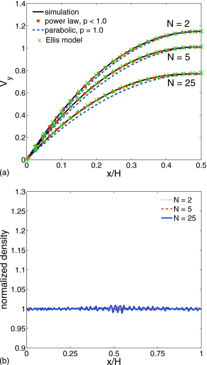
where p is the power-law index, κ is the power-law shear-stress coefficient, and n is the number density. Figure 3 shows velocity profiles (a) and normalized bead density (b) across the channel for chains of N=2, 5, and 25 beads driven by f=0.25. It also depicts excellent velocity-profile fits for the power law (dots) and for the Ellis model (crosses) with indices p=0.898 for N=2, p=0.831 for N=5, and p=0.703 for N=25 bead chains. For contrast, the parabolic Newtonian profiles (dashed lines) are also plotted with the non-Newtonian curves. The velocity profiles corresponding to the longer chains have smaller velocity maxima Vc and are flatter because these melts are more viscous and more strongly shear thinning (smaller p). In addition, Fig. 3b shows that the bead density distribution is essentially uniform for all monodisperse melts. The largest density deviations, within 1%–2% of the bulk density, were observed for the longest chains of N=25 near the centerline. Absent for this system of pure monodisperse chains is the cross-stream migration found for dilute and semidilute solutions.3, 21, 22, 23
Figure 3.
Velocity (a) and normalized bead density (b) profiles for three melts of N=2-, 5-, and 25-bead chains. Power-law indices p are 0.898, 0.831, and 0.703, respectively.
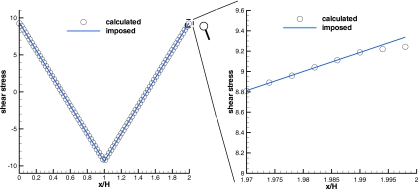
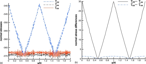
As a consistency test, Fig. 4 compares the imposed and the calculated shear-stress distributions for the melt of N=25 beads. Within the attainable statistical convergence, the overall agreement between the assigned and the calculated shear-stress distributions and the uniform density across the channel show that the system of monodisperse chains behaves as a homogeneous continuum. The small discrepancy in the near-wall region with thickness of less than 1% of the channel width H appears to be a consequence of the abrupt reversal of the driving force just beyond the wall. Repetition of this comparison for different driving forces showed this discrepancy to vanish as the driving force gets smaller. The periodicity of RPF suggests that as the ratio of particle size over H increases, this stress discrepancy will grow, and this may signal the breakdown of the continuum assumption. For the beads of this model, the Stokes–Einstein radius has been shown elsewhere4 to be a plausible measure of the particle size. Figure 5 shows the cross-channel distribution of normal-stress components (a) and normal-stress differences (b). The much larger fluctuations of the components imply the isotropic pressure to be nosier than the extra stress. This may be a consequence of averages taken in overly narrow subdivisions of the channel cross section, which are required to obtain the distributions. The subdivision size was chosen to obtain smooth velocity profiles. However, the average normal stresses appear to be noisier than both the velocity and the shear stresses plotted above, which suggests that a coarser discretization should be used for them.
Figure 4.
The calculated and imposed shear-stress distribution (left) for the melt of N=25 beads and the near-wall region (right, expanded scale).
Figure 5.
Profiles of normal stress components (a) and normal stress differences (b) for a melt of 25-bead chains driven by f=0.25.
The regularity assumptions of continuum theory allow for the expansion of V(x) in powers of x2, and for the low shear rates near the centerline, the leading terms are
| (10) |
This suggests that the central region of the velocity profile can be fitted well with even-order polynomials in x measured from the centerline, with the coefficient of x2 furnishing the zero-shear-rate viscosity η0. The calculation of the non-Newtonian viscosity and the normal-stress coefficients [Eq. 2] requires the distribution of the shear rate and the stress components τxy(x), τxx(x), τyy(x), and τzz(x) across the channel. For the viscosity, the noise-free imposed shear stress, τxy(x)=fn(H∕2−x) for x∊[0,H] and τxy(x)=fn(x−3H∕2) for x∊[H,2H], is preferred (see Fig. 1). For the normal-stress coefficients, the only option is the computed stress differences, i.e., Fig. 5, and hence they are necessarily noisier than the viscosity. The required shear rates are extracted from the calculated velocity profiles by numerical differentiation for which the straightforward approach is to use a simple finite-difference approximation for a uniform grid of spacing Δx, defined as xi=iΔx, i=0,…,M, where M=⌊0.5H∕Δx⌋. Constructed from the four-halves of the RPF, an ensemble-average velocity profile is then interpolated with cubic splines and projected onto the grid {xi}. This is appropriate for the near-wall region since polynomial interpolation is known to perform rather poorly for power-law functions [Eq. 9]. Shear rates at points xi+0.5 are then calculated from the second-order central difference (V(xi+1)−V(xi))∕Δx.
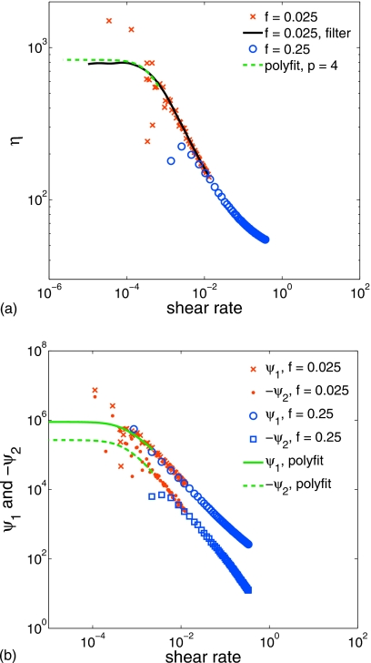
Figure 6 presents the shear-dependent viscosity (a) and the first and second normal-stress coefficients (b) for chains of N=25. The curves denoted by crosses and circles in Fig. 6 (a) display the shear-dependent viscosity obtained by the numerical differentiation described above. The plot shows clearly how direct numerical differentiation works very well except at the very low shear rates of the central region where large errors in the central-difference estimate of the derivative appear as scatter in the viscosity and the normal-stress coefficients [symbols in Fig. 6b]. This scatter was reduced by two methods: Firstly by filtering (smoothing) the original velocity data, and secondly by fits with low even-order polynomials. The solid line in Fig. 6a is the result of applying the Savitzky–Golay filter24 two to three times to the velocity data, followed by the direct numerical differentiation. While filtering substantially reduces the low shear-rate scatter, it tends to smooth out data peaks such as the centerline maximum velocity Vc. Consequently, the flattened profile leads to underprediction of the viscosity near the low shear-rate plateau, as can be seen in Fig. 6a. Smoothness for improved accuracy of differentiation in the low shear-rate neighborhood of the Poiseuille flow centerline was achieved with fits of low-order polynomials in the small neighborhood where the velocity profile should be nearly parabolic [Eq. 10]. The curves in Fig. 6 labeled “polyfit” employed a fourth-order polynomial fitted near the centerline by careful limitation of the region so that the term x4 is not dominant. For the higher driving force, f=0.25, the zero-shear-rate plateau cannot be obtained because the central region of the velocity profile is very narrow and not resolvable by fitting with low-order polynomials. Hence, full curves of viscosity and normal-stress coefficients for a particular system require at least two simulations: The first with a low driving force f to resolve the zero-shear viscosity plateau and, subsequently, one or more with higher f’s sufficient to provide overlapping resolution of the power-law region and possibly the high shear-rate plateau.
Figure 6.
The shear-dependent viscosity (a) and the first and second normal-stress coefficients (b) for 25-bead chains by direct numerical differentiation (symbols) and by curve filtering and fitting (solid and dashed lines).
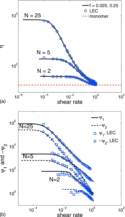
Figure 7 shows the shear-dependent viscosity (a) and the first and second normal-stress coefficients (b) for chains of N=2, 5, and 25 beads obtained by applying a combination of low-order polynomial fitting, filtering, and numerical differentiation as described above. For each melt the solid and dashed curves are the results from two simulations of RPF carried out with nondimensional forces f=0.025 and 0.25, respectively. The symbols in Fig. 7 denote analogous results obtained from simulations of plane Couette flow with LEC. The excellent agreement between the RPF and the LEC results over most of the shear-rate range suggests that the steady shear-rate properties of these monodisperse chains are material functions of the shear rate for any steady shear flow. Hence, these fluids appear to behave macroscopically as homogeneous simple fluids in the sense of Noll et al.25 The noticeable disagreement of the normal-stress coefficients for low shear rates, especially for two-bead chains, is associated with the errors of the small calculated normal-stress differences as they approach zero. For LEC these coefficients exhibit increasing scatter at shear rates below the points shown in Fig. 7b, while for RPF the same coefficients at low shear rates can be successfully extracted by use of local, low-order polynomial fits of the calculated normal-stress difference data. This procedure is similar to the fits of velocity profiles near the centerline described above. Since the normal-stress differences in that region have nearly flat distributions, it is essential to test the sensitivity of their coefficient plateaus to the chosen range of the fits.
Figure 7.
The shear dependent viscosity (a) and the first and second normal-stress coefficients (b) for chains of N=2, 5, 25 beads.
For two- and five-bead chains at very high shear rates, the LEC first normal-stress coefficient becomes negative. This unexpected feature was observed only for LEC simulations and not for comparable ones by RPF. Negative first normal stress coefficients are not expected for simple linear chains and appear to be artifacts of the LEC configuration. Although the smaller second normal stress coefficient does not change sign, the switch of the first for short chains only is an indication that the values may have become statistically insignificant. It is not clear why the corresponding Poiseuille flow with its stress gradient should be more stable than the uniformly stressed Couette flow. As stated previously, the stability of RPF relative to LEC at the extremes of the shear-rate domain may be a consequence of the different ways these flows are driven, namely, by a constant force on every particle versus by a prescribed wall velocity.
The integrated velocity profile [Eq. 9] is based on the assumption of a power-law shear-stress shear-rate relation for the entire channel. The viscosity functions exhibited in Fig. 7 clearly show the power-law region to lie between the upper and lower viscosity plateaus. The best estimate of the power p is then the slope 1−1∕p of the viscosity function taken at the inflection point. Table 2 shows that values of p derived from the viscosity function (p2) agree fairly well with those obtained from the velocity profile fits (p1). The table also shows asymptotic values of the mean relaxation time λ0=0.5ψ1∕η0 and the ratio −ψ2∕ψ1 as .
Table 2.
Power-law index p1 from velocity (Fig. 3) and p2 from viscosity (Fig. 7), the zero-shear-rate viscosity η0, the mean relaxation time λ0, and the normal stress coefficients ratio.
| N | p1 | p2 | η0 | λ0 | −ψ2∕ψ1 |
|---|---|---|---|---|---|
| 2 | 0.898 | 0.89 | 62.7 | 0.636 | 0.003 |
| 5 | 0.831 | 0.81 | 138.4 | 8.564 | 0.281 |
| 25 | 0.703 | 0.68 | 830.9 | 536.73 | 0.3 |
Remarkably, all viscosity curves in Fig. 7a converge at high shear rates to the same plateau, which corresponds to the Newtonian viscosity of the DPD fluid of unchained or free beads (monomers) having the same density and with the same interparticle forces. Figure 8 shows snapshots from visualizations of single, marked chains moving within melts of unmarked chains at low shear rates (a) and high shear rates (b). At low shear rates, the chains are entangled across the shear planes, whereas at high shear rates, they tend to completely disentangle and are drawn out along and are convected within the unstretchable shear planes. This implies a passive role for the spring connectors at high shear rates and suggests why the monomer viscosity is the common plateau value for all N (the complete visualizations can be viewed in supplemental materials which show larger amplitudes for fluctuations at low shear rates than for high shear rates). Thus, in steady shear flow a typical chain behaves as follows: It stretches along the shear planes and then tumbles. At high shear rates, the tumble is constrained mostly within the shear planes so that the reversal of chain ends occurs within the same shear plane. The residence time for the stretching stage depends on the shear rate, bead interactions, and most importantly, the chain length. While at low shear rates, where fluctuations are dominant, the chain ends are frequently impelled across the shear planes, and their near-equilibrium entanglements reach across to neighboring planes with different average velocities.
Figure 8.
Collage of snapshots of a single 25-bead chain within a melt of unmarked chains at low shear rates (a) and at high shear rates (b) plotted on the same scale. Constant x defines the shear planes. (Enhanced online.)
Each symbol in Fig. 7 corresponds to one LEC simulation for each prescribed shear rate. In this case, even though the computational domain for all LEC simulations was 10×10×10 in DPD units or ten times smaller by volume than the RPF domain, the total computational expense for the full material functions of comparable accuracy is several times larger for LEC than for RPF. Clearly, this depends on the number of LEC shear rates deemed necessary to define the curves, and in Fig. 7 that number may be excessive. In addition, statistical averaging of LEC stresses requires longer running times than those for RPF which combine both time and ensemble averages. Thus, the apparent advantage of an imposed shear rate in LEC is offset by the higher noise levels of the stresses. In RPF the shear-stress distribution is prescribed, and the shear rate must then be determined by numerical differentiation of the velocity profile. The latter operation turns out to be less noisy than the stress calculation because the statistical convergence of the velocity is more accurate and smoother than that of the stresses. This implies greater accuracy for the RPF viscosity function than for its normal-stress coefficients. A further advantage of RPF capability is to more easily extract the low shear-rate plateaus of the material functions. As a rheometer, RPF performs similar to experimental real steady-shear rheometers for which it is generally true that the viscosity function is more accurately measured than the normal-stress functions. Likewise the measurement of the low shear-rate plateaus is nearly always restricted by the limits of instrumental detection.
The properties of the model fluids of monodisperse chains, introduced above as melts, can now be compared with those of real melts. The viscosity data of a homologous series of undiluted polystyrenes with narrow molecular weight distributions26 exhibit a common power law over a fivefold range of molecular weights even though η0 varies by several orders of magnitude. Hence, the power-law exponents in Table 2 suggest that if the models of this work are taken to represent whole polymers, the bead number N alone is not a satisfactory proxy for molecular weight. In preliminary simulations the fluids of bead-spring chains were investigated with the cutoff radius rc set to 1, and the resulting viscosity functions were found to be only slightly non-Newtonian. Since the number of neighbor interactions increases as , this shows the sensitivity of non-Newtonian response for such models. Thus, it should be possible to adjust model parameters to yield a series of fluids of monodisperse bead-spring chains with power-law indices independent of N, in agreement with the experiment. However, this amounts to an ad hoc variation in the viscosity of the “monomer” fluids, and its validity would need to be tested for consistency against other properties. The untangling visualized in Fig. 8 at high shear rates is not thought to occur for real polymers. Even though the data in Ref. 26, typical for whole polymers, do not extend beyond the power-law regime, it is usually accepted that at high shear rates these materials will exhibit a glassy response. Clearly, the simplistic models employed in this work describe at best the rubbery regime. In spite of these limitations, the ratios −ψ2∕ψ1 as in Table 2 are very close to the reptation theory prediction of 2∕7,27 except for N=2. The second normal-stress difference for two-bead chains is very small at low shear rates, and the discrepancy of the ratio suggests that either the limit of detection has been reached or that dumbbells are a poor representation of a polymer.
Finally, DPD time scales can be related to those of real polymer fluids from the observation that for both monodisperse and polydisperse melts, the transition from the low shear-rate plateaus to the power-law regime occurs at shear rates , e.g., polystyrenes26 and polyethylenes,27 respectively. This is also true for the simulated viscosity functions of this work; hence, matching of λ0’s relates the real and the DPD time scales. Normal-stress data for monodisperse melts may be difficult to obtain,28, 29 and the alternative is to derive λ0 from low-frequency dynamic-modulus measurements.
Solutions
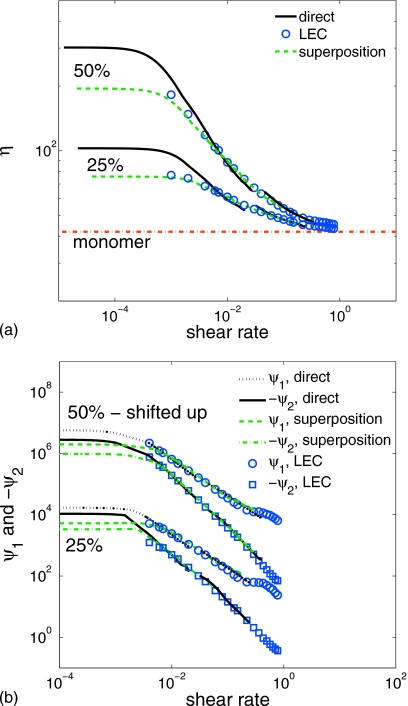
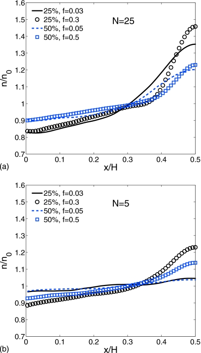
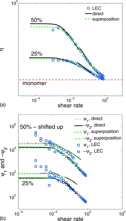
In this section the steady shear material functions are calculated for solutions of the bead-spring chains in solvents of free DPD particles. Two concentrations, 25% and 50%, were simulated for monodisperse chains of 5 and 25 beads, respectively. Since the chain beads and the free solvent particles have the same mass, the chain-bead number density or concentration n is also the chain mass concentration. The free particles constitute a good solvent since their force interaction parameters are identical to those of the chain beads. The simulation parameters are outlined in Table 1, and the RPF computational domain is identical to the one described in Sec. 4A. Two simulations for each solution were carried out with imposed nondimensional body forces f=0.03 and 0.3 for the 25% solutions, and f=0.05 and 0.5 for the 50% solutions, respectively. Corresponding LEC simulations were also carried out over the same range of shear rates. Figure 9 shows the shear-dependent viscosity (a) and the first and second normal-stress coefficients (b) for the solution of N=25-bead chains at concentrations of 25% and 50%. The symbols in Fig. 9 stand for the LEC simulations of the same solutions, and the curves labeled as “direct” are extracted from the RPF simulations with local low-order interpolation, filtering and numerical differentiation, as described above in Sec. 4A. Here, the disagreement between RPF and LEC results is noticeable with different zero-shear-rate viscosities and distinctive slopes in the power-law region. Macroscopic theories of mixtures suggest that the concentration should be uniform in the absence of stress gradients. Consequently, plane Couette flow should yield results free from concentration gradient effects. In all LEC simulations, the concentration was found to be uniform, whereas in RPF, the concentration distributions were found to be nonuniform. This behavior is attributed to the stress gradient across the channel.
Figure 9.
Shear dependent viscosity (a) and first and second normal-stress coefficients (b) for solutions of N=25-bead chains at mass concentrations of 25% and 50%. The 50% curves in the lower figure have been “shifted up” two orders of magnitude for visual clarity.
Figure 10 presents the chain-bead densities across the channel normalized by their bulk values, for 25-bead solutions (a) and for 5-bead solutions (b) for two driving forces at each concentration. The effect of the Poiseuille stress gradient is a steeper and more confined concentration distribution in the central region for longer chains (N=25), higher body forces, and smaller chain-bead concentrations (25%). Figure 9 indicates higher viscosities relative to the LEC values in the lower shear-rate central region where the local concentration exceeds the bulk value, and vice versa, in the high shear-rate wall region where the local concentration is depleted relative to the bulk value. The steady shear-rate material functions of real polymer solutions are known to depend on both shear rate and concentration. At different concentrations, polymer properties usually correlate by means of the empirical principle of time-concentration superposition which requires both the dependent and the independent variables to scale according to certain rules. In particular, the concentration dependence is determined by that of the zero-shear-rate viscosity of the solution η0 relative to the Newtonian solvent viscosity ηs. For concentrated solutions, this difference is assumed to be of the form,30
| (11) |
where n is the mass concentration (chain-bead number density here), [η]0 is the intrinsic zero-shear-rate viscosity, and k′ is an arbitrary constant. It is assumed that [η]0∼Ma, where M is the molecular weight and a is a power depending on the critical molecular weight. Thus, [η]0 is constant for a given polymer and is also taken as such for the model chains of 5 and 25 beads. The superposition shift factor is formed as
| (12) |
where α=k′[η]0. Note that an is the shift factor only for η−ηs, and hence, the total shifted viscosity is (η−ηs)an+ηs, whereas the normal-stress coefficients are shifted as and , and the shear rate as .
Figure 10.
Normalized chain-bead number density distributions for 25-bead (a) and 5-bead solutions (b) for different bulk concentrations n0 and body forces f.
Here, we examine whether this principle applies to the DPD solutions described above and, in particular, whether the solid direct curves in Fig. 9, being discontinuous in the transition from the smaller to the larger f, can be reconciled to lie on a single curve in agreement with the LEC points. Returning to Fig. 9, the curves denoted as “superposition” were obtained from the local concentration (Fig. 10) and the superposition shift factor an with α=1.5. The α value was found by superposition of LEC curves at the two concentrations (not shown). In the absence of LEC results, α can be found by imposition of continuity on the shifted RPF results for different driving forces to yield the superposition curves in Fig. 9. The superposed RPF curves are continuous and agree well with the LEC points, and thus, the principle of time-concentration superposition applies to the model solutions of 25-bead chains. Although large concentration gradients would appear to negate the use of the RPF configuration as a rheometer, useful measurements of bulk solution properties can be obtained when concentration superposition is applicable.
For the five-bead chain solutions, Fig. 11 shows that the time-concentration superposition as implemented above yields satisfactory results for the viscosity, and the second normal stress coefficient, but with some inconsistency between LEC and RPF for the first normal stress coefficient. As expected, the smaller concentration gradients (Fig. 10) relative to N=25 reduce the deviations of the direct viscosity curves from the LEC points and their discontinuities are smaller than their N=25 counterparts in Fig. 9a. Here, the time-concentration superposition, as described above, was applied with α=0.75 to yield excellent agreement between the LEC points and the RPF viscosity superposition curves. Note the scatter in the LEC points for the normal-stress coefficients at low shear rates. The surprising result is the behavior of the first normal-stress coefficient for which the LEC points decay faster with shear rate relative to the superposed RPF curves, and that the disagreement is worse for the more dilute 25% solution. Eventually, ψ1 by LEC becomes negative (not shown), while agreement between the second normal-stress coefficients remains very close. This artifact of the Couette flow appears to be a short-chain phenomenon, having been seen above for the two- and five-bead melts and is more pronounced here for the 25% solution of five-bead chains.
Figure 11.
Shear dependent viscosity (a) and first and second normal-stress coefficients (b) for solutions of five-bead chains at mass concentrations 25% and 50%. The 50% curves in the lower figure have been shifted up two orders of magnitude for visual clarity.
The large concentration changes across the channel indicate that the simulated solutions do not capture the diffusion rates of real polymer solutions. Cross-stream migration effects of this magnitude are not known for polymer solutions flowing in channels of laboratory length scales. An alternative interpretation is that the nonuniform concentration distributions are a manifestation of size effects since the channel width is only twice the fully extended length of the longest chain. The distributions of Fig. 10 reveal the concentration peaks to be higher for the longer chains, which indicates that the width H is a microchannel scale for these chains.
Finally, Table 3 gives the power-law indices and zero-shear-rate properties for the solutions of chains N=5 and 25 beads at different concentrations. Here again, the mean relaxation time λ0 defines the characteristic time scale for the DPD solutions and which is much smaller for short chains. The ratio −ψ2∕ψ1 for all solutions is larger than the value of 2∕7 predicted by the reptation theory27 for undiluted polymers. For the five-bead chains, the values of the second normal-stress coefficient may be at the limit of statistical significance as .
Table 3.
Power-law indices and zero-shear-rate properties for solutions of N=5- and 25-bead chains at two concentrations.
| N | Concentration (%) | p | η0 | λ0 | −ψ2∕ψ1 |
|---|---|---|---|---|---|
| 5 | 25 | 0.95 | 53.2 | 0.924 | 0.39 |
| 5 | 50 | 0.9 | 76.5 | 2.26 | 0.43 |
| 25 | 25 | 0.89 | 75.8 | 34.7 | 0.63 |
| 25 | 50 | 0.78 | 194.5 | 50.7 | 0.49 |
Temperature dependence of rheological properties
In view of the success of superposition to account for concentration effects, the temperature dependence of the steady shear-rate properties of monodisperse bead-chain melts will also be treated by the principle of superposition. Time-temperature superposition is a well established, but mainly empirical, procedure31 widely employed for real polymer materials. The scaling of both the dependent and the independent variables can be motivated by polymer theories at the mesoscopic level, such as the Rouse theory.27, 31 Generally, in these theories, including that of rubber elasticity, the equilibrium Helmholtz free energy is athermal, i.e., linear in kBT. This implies that the entropy is entirely configurational or independent of kBT, and thus the equation of state for the equilibrium pressure p must be of the form
| (13) |
Here, the second equality follows from the additional assumption that f(n) has a virial expansion whose coefficients bi must be constant, the best-known example being the hard sphere gas. For molecules with spherical symmetry, constant virial coefficients are a consequence of temperature-independent radial-distribution functions (RDFs).32
For the DPD fluids of this work, the contribution to the excess pressure is calculated from the virial theorem as
| (14) |
where the forces were defined above in Sec. 3. For a fluid of free DPD particles at densities well beyond the ideal gas regime, Groot and Warren17 found from simulations the equation of state to be approximately p=nkBT+c2n2, where c2 is a constant proportional to the conservative force coefficient a. The equation of state found by Groot and Warren17 is not a truncated virial expansion about the ideal gas state. Thus, c2 is not the second virial coefficient as implied by the second equality of Eq. 13. Pagonabarraga and Frenkel33, 34 derived this result with multibody DPD (an enhanced version of the standard two-body DPD employed here). However, Groot and Warren’s simulations covered only one isotherm, and hence, the temperature dependence of a was not considered.
Statistical mechanics provides examples of mesoscopic forces whose expressions carry the prefix kBT. Here, the relevant one is the Langevin force on a tethered chain, of which the FENE force30 is an approximation. Since DPD beads are point particles which represent loose aggregates of many molecules it is plausible to assume their soft potentials also have the kBT hallmark of mesoscopic forces. Indeed, Eq. 14 suggests the equation of state will have the athermal form of the first equality of Eq. 13 provided both the conservative force coefficient a and the spring constant ks are linear in kBT,
| (15) |
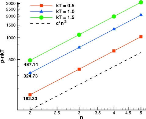
where a0 and ks0 are the reference parameters corresponding to temperature kBT=1. This was verified with equilibrium simulations of a melt of five-bead chains over a range of bead densities n at three temperatures kBT=0.5, 1.0, and 1.5. The temperature was set by adjustment of the dissipative force coefficient according to γ=γ0∕kBT, which from Eq. 6 means that σ was held constant. Table 4 summarizes the constant DPD parameters specified for simulations. Figure 12 shows the excess equilibrium pressure versus bead density at several temperatures simulated with the parameter scaling of Eq. 15. For n≥2, the curves for different temperatures clearly plot as parallel lines on logarithmic scales and shift onto a single line by scaling the excess pressure with temperature. It is easily verified that the excess pressures at n=2 satisfy 487.14∕1.5≈324.73≈162.33∕0.5. In Fig. 12 the dashed reference line has slope of 2 to show that the form of the equation of state of Groot and Warren17 for free beads also holds for the bead-chain models provided the conservative force coefficient scales according to Eq. 15. Although not shown here, the RDF for these melts was verified to be independent of temperature which demonstrates the temperature-independent structure requirement of the athermal fluid.
Table 4.
DPD parameters for RPF simulations.
| rc | a0 | γ0 | σ | m [Eq. 7] | ks0 | rmax |
|---|---|---|---|---|---|---|
| 2.0 | 50.0 | 4.5 | 3.0 | 0.25 | 100.0 | 2.0 |
Figure 12.
log-log plot of the excess equilibrium pressure for different bead densities at several temperatures. Melts of five-bead chains.
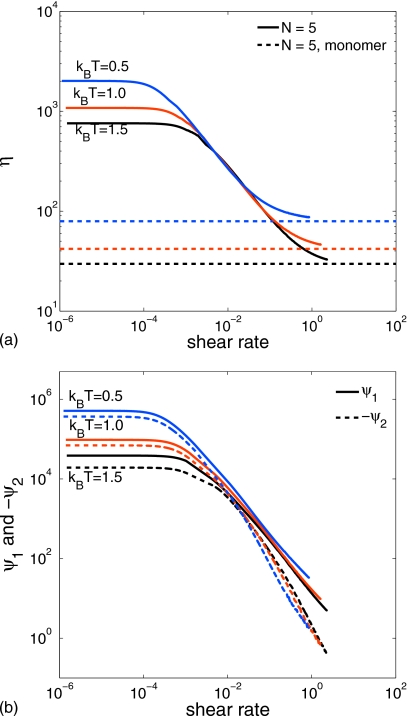
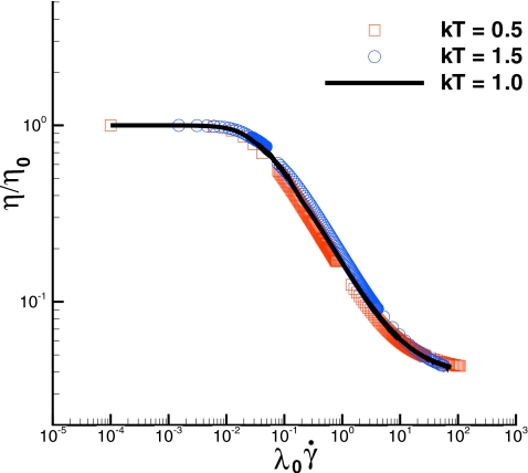
For the melt of five-bead chains with bead density n=3, RPF simulations were carried out at three temperatures, kBT=0.5, 1.0, and 1.5 in a 50×20×10 box, with the constant simulation parameters given in Table 4. To capture both the low and the high shear-rate plateaus of the viscosity function at each temperature, runs were carried out for three nondimensional body forces f=0.025, 0.25, and 1.0. Figure 13 shows the resulting shear-dependent viscosity (a) and the first and second normal-stress coefficients (b) at the three temperatures. Visual inspection of the shapes of these bilogarithmic plots suggests that the curves can be superposed. Indeed, when the ordinates are normalized by their zero-shear-rate values, and the shear rates are multiplied by the factor aT=γ(T)∕γ(T0)η0(T0)∕η0(T), then all the curves shift onto the kBT=1.0 curve. The superpositions are not shown since the deviations from the common curve are not visible on the scale of Fig. 13.
Figure 13.
The viscosity function (a) and the first and second normal-stress coefficients (b) at three temperatures for five-bead chains.
For real polymers, the shift factor is generally taken to be aT=η0(T0)∕η0(T). No rigorous argument can be given for including the dissipative force coefficient in the shear-rate shift factor. However, γ (dimension time−1) is proportional to a time scale of the DPD system, and therefore this empiricism is not entirely surprising. Since γ is not measurable experimentally, an alternative scaling is employed in Fig. 14. Here, the viscosities are normalized by their zero-shear-rate values η0, and the shear rate is rendered dimensionless with the mean relaxation time λ0 from Table 5. This scaling was used by Graessley et al.28 to correlate viscosity data for nearly monodisperse polystyrenes. Table 5 gives the power-law indices and the low shear-rate properties at the three temperatures. The temperature independence of the power-law index agrees with experimental experience for monodisperse polystyrenes.28 Compared to the five-bead melt in Fig. 7 (Sec. 4A), the five-bead melt at kBT=1.0 in Fig. 13 exhibits a much stronger shear thinning. The difference between these chains and those in Fig. 7 is the doubling here of rmax, and hence of the fully extended contour length. This points to contour length rather than bead number as the chain property that mainly determines the steepness of the viscosity function. Section 2 discusses the difficulties of extracting accurate zero-shear-rate values of the material functions; Fig. 14 suggests that they are quite accurate, otherwise the superposed curves would tend to separate.
Figure 14.
The time-temperature superposition of the shear-dependent viscosity for five-bead chain melts at three temperatures.
Table 5.
The power-law indices and zero-shear-rate properties for three temperatures.
| kBT | p | η0 | λ0 | −ψ2∕ψ1 |
|---|---|---|---|---|
| 0.5 | 0.665 | 2015.2 | 128 | 0.7 |
| 1.0 | 0.665 | 1082.4 | 44.5 | 0.7 |
| 1.5 | 0.665 | 757.8 | 25.4 | 0.5 |
Although the athermal equation of state is a restricted idealization, it is critical to the definition of a DPD model which will satisfy time-temperature superposition. The results (not shown) for simulations carried out with beads having constant conservative force coefficients a did not satisfy the time-superposition principle. The temperature range over which real polymers are studied is much smaller than the simulated threefold change in Fig. 14, and thus the athermal approximation of the equation of state may then become plausible over the short temperature range of interest.
SUMMARY
Numerical statistical mechanics is motivated by the need to study those systems for which analytical statistics yields no results. With DPD, as with other particle-based models, the study of a new model begins with the assumption of particle forces and structures to represent the “molecules” or microstructure. The test of a model is the verification of its macroscopic properties relative to those measured for real materials, and for this purpose, virtual rheometers are needed to simulate numerical tests similar to the experimental tests performed in the laboratory by rheologists. In this work, the material functions of steady-state shear flow for some simple models of complex fluids have been calculated with a novel variant of plane channel flow, RPF, and with the commonly used uniform shear flow with LEC.
In each of these virtual rheometers, periodic boundary conditions avoid the need to model real solid boundary conditions with their known pitfalls, and this implies that the calculated properties are bulk values for both RPF and LEC. This is confirmed for a fluid of monodisperse chains in Fig. 3, where the RPF bead density distribution is shown to be uniform across the channel section, and in Fig. 4 where the shear stress calculated from the simulation data by the Irving–Kirkwood equation is shown to be consistent with the imposed shear-stress distribution determined from the continuum equation of motion. The uniformity of density and stress in LEC was checked, but is not shown. The reversal of the driving force over half the RPF computational domain guarantees zero mean velocity on the dividing shear plane, which provides a way to check hypotheses for wall boundary conditions in channels with real walls.
The results presented above demonstrate that shear-rate dependent properties of model DPD fluids can be accurately determined with the RPF rheometer, and how the latter complements, confirms, and extends the results obtained with LEC. Continuum theory requires these shear-rate dependent properties to be material functions of the shear rate, independent of the type of shear flow. Examples of experimental data conforming to this requirement are given in Ref. 25. This requirement is also satisfied for the simple DPD models investigated here, for instance, Fig. 7, which indicates they are continuum fluids. The concentration and temperature dependence of their calculated material functions were also found to be consistent with the empirical principles of concentration and temperature superposition satisfied by most real polymer fluids. Furthermore, time-concentration superposition was demonstrated for solutions of flexible chains with concentration gradients (see Figs. 911). This implies that for the systems of this work the steady shear-rate material functions depend only on the local temperature, concentration, and shear rate.
During the course of this work, it was found that RPF has some advantages over the conventional LEC configuration. Firstly, the latter determines material-function values for only one shear rate per simulation, whereas a single RPF simulation yields the same data for a wide range of shear rates from zero at the centerline to the wall value. This efficiency appears to be negated by the extra data analysis, which is demanded by the spatially varying shear rate; however, the numerical differentiation of the velocity field is conveniently implemented with standard packages such as MATLAB. The computational domain of the RPF configuration used here is several times larger than the LECs. The determination of the smallest, and hence most economical, satisfactory RPF domain is left for future work. Secondly, RPF yields more complete rheograms than those computed from LEC alone. In particular, near the zero-shear-rate plateaus RPF values are smooth, whereas LEC results tend toward increased scatter. Likewise, at the highest shear rates first normal stress differences by LEC unexpectedly change sign, while the corresponding RPF values remain positive. It is inherent in DPD that at the low shear-rate extreme the thermal fluctuations overwhelm the steady-state dynamic properties, and that at the highest rates, viscous dissipation overwhelms the thermostat. The stability at the extremes of RPF relative to LEC is not easily explained, but it may be a reflection of the way these flows are driven: A uniform body force applied on every particle versus a uniform velocity applied on the boundary, respectively. This hypothesis could be investigated with the DOLLS (Ref. 35) or the SLLOD (Ref. 36) algorithms in which the Couette flow is driven by body forces in contrast to the boundary-driven LEC algorithm. The smoothness of the channel profiles of both velocity and stress derived from RPF appears to be a consequence of the fourfold ensemble averaging over half-channels inherent in the configuration. The unexpected conclusion of this work is that viscosities obtained by numerical differentiation of the RPF velocity distribution combined with the prescribed shear stress are often a less noisy operation than the prescribed shear rate of LEC combined with calculated shear stress. Since the RPF normal stress differences are not prescribed, they are necessarily noisier than the shear stress, but still benefit from the inherent smoothness of RPF.
The fluid models composed of monodisperse chains, referred to as melts, were shown to have steady shear-rate material functions of forms typical of polymer fluids. These functions were found to satisfy the principle of time-temperature superposition only when all the bead forces have a linear dependence on temperature, which is a characteristic of mesoscopic forces. This has been long understood for the force-extension relations for chains derived from statistical mechanics, but not explicitly for the soft potentials of DPD beads, which are usually studied at only one temperature. At equilibrium, these melts were shown to satisfy an athermal equation of state, i.e., their entropy is purely configurational. However, in their present form these models only partially capture the behavior of real monodisperse polymer melts and solutions. In particular, the tendency for complete disentanglement of chains at high shear rates does not correspond to what little is known for real polymers; data are rare at shear rates approaching the upper plateau viscosity. To bring the model predictions into quantitative correspondence with the response of real polymer fluids requires a deeper understanding of the coarse graining of real polymer chains into bead-chain systems. The examples of this work demonstrate that the steady shear response of a polymer model can efficiently yield important insights into its adequacy without the need for a costly, complete rheological characterization. Hence, RPF used in conjunction with LEC is a useful tool for the assessment of new and improved models.
ACKNOWLEDGMENTS
This work was supported by NSF∕CBET and by NIH. Simulations were performed on the TACC Ranger and NICS Kraken supercomputing systems sponsored by NSF.
References
- Backer J. A., Lowe C. P., Hoefsloot H. C. J., and Iedema P. D., J. Chem. Phys. 122, 154503 (2005). 10.1063/1.1883163 [DOI] [PubMed] [Google Scholar]
- Lees A. W. and Edwards S. F., J. Phys. C 5, 1921 (1972). 10.1088/0022-3719/5/15/006 [DOI] [Google Scholar]
- Fedosov D. A., Karniadakis G. E., and Caswell B., J. Chem. Phys. 128, 144903 (2008). 10.1063/1.2897761 [DOI] [PubMed] [Google Scholar]
- Pan W., Ph.D. thesis, Brown University, 2010. [Google Scholar]
- Einstein A., Investigations on the Theory of the Brownian Movement (Dover, New York, 1956). [Google Scholar]
- Batchelor G. K., J. Fluid Mech. 83, 97 (1977). 10.1017/S0022112077001062 [DOI] [Google Scholar]
- Bicerano J., Douglas J. F., and Brune D. A., J. Macromol. Sci., Rev. Macromol. Chem. Phys. 39, 561 (1999). [Google Scholar]
- Chong J. S., Christiansen E. B., and Baer A. D., J. Appl. Polym. Sci. 15, 2007 (1971). 10.1002/app.1971.070150818 [DOI] [Google Scholar]
- Ferrini F., Ercolani D., and Cindio B. D., Rheol. Acta 18, 289 (1979). 10.1007/BF01542776 [DOI] [Google Scholar]
- Poslinski A. J., Ryan M. E., Gupta P. K., Seshadri S. G., and Frechette F. J., J. Rheol. 32, 751 (1988). 10.1122/1.549991 [DOI] [Google Scholar]
- Storms R. F., Ramarao B. V., and Weiland R. H., Powder Technol. 63, 247 (1990). 10.1016/0032-5910(90)80050-9 [DOI] [Google Scholar]
- Shikata T. and Pearson D. S., J. Rheol. 38, 601 (1994). 10.1122/1.550477 [DOI] [Google Scholar]
- Chang C. and Powell R. L., J. Rheol. 38, 85 (1994). 10.1122/1.550497 [DOI] [Google Scholar]
- Irving J. H. and Kirkwood J. G., J. Chem. Phys. 18, 817 (1950). 10.1063/1.1747782 [DOI] [Google Scholar]
- Cray C. G. and Gubbins K. I., Theory of Molecular Fluids (Clarendon, Oxford, 1982). [Google Scholar]
- Hoogerbrugge P. J. and Koelman J. M. V. A., Europhys. Lett. 19, 155 (1992). 10.1209/0295-5075/19/3/001 [DOI] [Google Scholar]
- Groot R. D. and Warren P. B., J. Chem. Phys. 107, 4423 (1997). 10.1063/1.474784 [DOI] [Google Scholar]
- Español P. and Warren P., Europhys. Lett. 30, 191 (1995). 10.1209/0295-5075/30/4/001 [DOI] [Google Scholar]
- Fan X., Phan-Thien N., Chen S., Wu X., and Ng T. Y., Phys. Fluids 18, 063102 (2006). 10.1063/1.2206595 [DOI] [Google Scholar]
- Symeonidis V., Caswell B., and Karniadakis G. E., J. Chem. Phys. 125, 184902 (2006). 10.1063/1.2360274 [DOI] [PubMed] [Google Scholar]
- Usta O. B., Butler J. E., and Ladd A. J. C., Phys. Fluids 18, 031703 (2006). 10.1063/1.2186591 [DOI] [Google Scholar]
- Chen Y. -L., Ma H., Graham M. D., and de Pablo J. J., Macromolecules 40, 85 (2007). [Google Scholar]
- Khare R., Graham M. D., and de Pablo J. J., Phys. Rev. Lett. 96, 224505 (2006). 10.1103/PhysRevLett.96.224505 [DOI] [PubMed] [Google Scholar]
- Orfanidis S. J., Introduction to Signal Processing (Prentice-Hall, Englewood Cliffs, NJ, 1996). [Google Scholar]
- Coleman B. D., Markovitz H., and Noll W., Viscometric Flows of Non-Newtonian Fluids (Springer-Verlag, New York, 1966). [Google Scholar]
- Graessley W. W., Advances in Polymer Science (Springer-Verlag, New York, 1974). [Google Scholar]
- Larson R. G., The Structure and Rheology of Complex Fluids (Oxford University Press, Oxford, NY, 1999). [Google Scholar]
- Mark J., Ngai K., Graessley W., Mandelkern L., Samulski E., Koenig J., and Wignall G., Physical Properties of Polymers, 3rd ed. (Cambridge University Press, Cambridge, 2004). [Google Scholar]
- Schweizer T., Hosettler J., and Mettler F., Rheol. Acta 47, 943 (2008). 10.1007/s00397-008-0300-5 [DOI] [Google Scholar]
- Bird R. B., Armstrong R. C., and Hassager O., Dynamics of Polymeric Liquids: Fluid Mechanics, 2nd ed. (Wiley, New York, 1987). [Google Scholar]
- Ferry J. D., Viscoelastic Properties of Polymers, 3rd ed. (Wiley, New York, 1980). [Google Scholar]
- McQuarrie D. A., Statistical Mechanics (Viva Books Private Limited, New Delhi, India, 2000). [Google Scholar]
- Pagonabarraga I. and Frenkel D., Mol. Simul. 25, 167 (2000). 10.1080/08927020008044122 [DOI] [Google Scholar]
- Pagonabarraga I. and Frenkel D., J. Chem. Phys. 115, 5015 (2001). 10.1063/1.1396848 [DOI] [Google Scholar]
- Hoover W. G., Evans D. J., Hickman R. B., Ladd A. J. C., Ashurst W. T., and Moran B., Phys. Rev. A 22, 1690 (1980). 10.1103/PhysRevA.22.1690 [DOI] [Google Scholar]
- Evans D. J. and Morriss G. P., Phys. Rev. A 30, 1528 (1984). 10.1103/PhysRevA.30.1528 [DOI] [Google Scholar]


