Sedimentation Patterns of Rapidly Reversible Protein Interactions

Abstract

The transport behavior of macromolecular mixtures with rapidly reversible complex formation is of great interest in the study of protein interactions by many different methods. Complicated transport patterns arise even for simple bimolecular reactions, when all species exhibit different migration velocities. Although partial differential equations are available to describe the spatial and temporal evolution of the interacting system given particular initial conditions, a general overview of the phase behavior of the systems in parameter space has not yet been reported. In the case of sedimentation of two-component mixtures, this study presents simple analytical solutions that solve the underlying equations in the diffusion-free limit previously subject to Gilbert-Jenkins theory. The new expressions describe, with high precision, the average sedimentation coefficients and composition of each boundary, which allow the examination of features of the whole parameter space at once, and may be used for experimental design and robust analysis of experimental boundary patterns to derive the stoichiometry and affinity of the complex. This study finds previously unrecognized features, including a phase transition between boundary patterns. The model reveals that the time-average velocities of all components in the reaction mixture must match—a condition that suggests an intuitive physical picture of an effective particle of the coupled cosedimentation of an interacting system. Adding to the existing numerical solutions of the relevant partial differential equations, the effective particle model provides physical insights into the relationships of the parameters that govern sedimentation patterns.

Introduction

Nontrivial patterns arise in the transport of rapidly reversible systems of interacting macromolecules when the lifetime of the complexes is short relative to a characteristic transport time of the experiment, such that all species remain locally in chemical equilibrium despite their spatial migration at different velocities. This topic is still of great importance, as dynamically associating and dissociating (multi-) protein complexes with short lifetimes are a ubiquitous motif of cellular regulation and biological signal transduction pathways, and many biophysical techniques rely on the observation of the cotransport of bound molecules.

This work focuses on the sedimentation behavior of such systems arising in two-component mixtures, as observed in sedimentation velocity (SV) analytical ultracentrifugation. With the introduction of modern instrumentation and computational methods, SV analytical ultracentrifugation has reemerged in the last decade as a powerful tool with broad applications in structural biology, biochemistry, immunology, biotechnology, and nanotechnology. In particular, there has been a strong increase in interest in using SV analytical ultracentrifugation to examine interacting systems. Because the experimental configuration of SV permits the hydrodynamic discrimination of boundaries containing complexes while they stay immersed in the slower-sedimenting constituents (Fig. 1, top), SV offers a unique potential for characterizing reversibly interacting macromolecules with regard to the number, stoichiometry, and binding constant of complex formation, as well as the low-resolution conformation of the complex.

Figure 1.

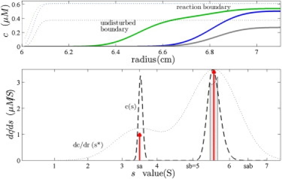
(Top) Concentration profiles calculated from Lamm PDE solutions for species A (3.5 S, green) reversibly interacting with B (5 S, blue) to form transient complexes AB (6.5 S, gray), sedimenting at 60,000 rpm. Initially, c_Atot(r,t = 0) = c_Btot(r,t = 0) = K_D, and shown are c_k(r,t) at 5 min (dotted) and t^∗ = 100 min (solid lines). (Bottom) Experimentally, from the measured total signal, c_Atot(r,t^∗) + c_Btot(r,t^∗) could be easily determined an apparent velocity distribution g^∗(s^∗) ∼ dc/dr (dotted line), or the diffusion-deconvoluted sedimentation coefficient distribution c(s) (23) (dashed line). The asymptotic boundary $d\widehat{c}/ds$ from GJT is shown as a light gray bar, and the predictions from EPT are shown as red arrows (scaled to represent the relative signal amplitudes, assuming equal signal increments).

So far, the prediction of the temporal and spatial concentration profiles that occur in the sedimentation process has been amenable largely only to numerical solutions of the coupled reaction and transport equations. In a seminal work in the 1950s, Gilbert and Jenkins solved (iteratively) the equations of cotransport of reacting systems in a diffusion-free approximation (1,2). This simplification highlights the salient features of the process: for rapidly reacting two-component systems, the Gilbert-Jenkins theory (GJT) explains the occurrence of a monodisperse undisturbed boundary and a polydisperse reaction boundary (also referred to as asymptotic boundary; see Fig. 1, bottom). It makes provocative predictions for both—among them that the undisturbed boundary migrates with the velocity of one of the free species, but it is neither always the one sedimenting slower, nor always the component in molar excess. Another prediction is that the reaction boundary exhibits a concentration-dependent range of migration velocities in between that of the faster sedimenting component and the complex species, but the overall velocity of the reaction boundary does not necessarily increase with increasing total concentrations (Fig. 2, bottom).

Figure 2.

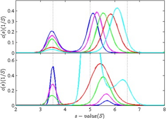
Sedimentation coefficient distributions c(s) representing the boundary patterns of the interacting system of Fig. 1 at different total loading concentrations. The vertical lines indicate the s values of the free and complex species. (Top) Dilution series with equimolar concentrations at 0.1 K_D (blue), 0.3 K_D (pink), K_D (green), 3 K_D (red), and 10 K_D (cyan). The c(s) distributions are normalized relative to the total loading concentrations. (Bottom) Titration series of a constant total concentration c_Atot= K_D of the smaller species A with increasing concentrations c_Btot of 0.1 K_D (blue), 0.3 K_D (pink), K_D (green), 2.366 K_D (red), and 10 K_D (cyan). Distributions are not normalized. For both panels, sedimentation and reaction parameters are as in Fig. 1, with signal coefficients of 40,000 M⁻¹ cm⁻¹ and 60,000 M⁻¹ cm⁻¹ for A and B, respectively.

The GJT is widely accepted and experimentally confirmed, and has remained highly influential to this date. It has been applied similarly to electrophoresis and size-exclusion chromatography of interacting systems (3–5) and its principles were generalized to other physical macromolecular interactions (6). However, due to the complexity of the approach, very few applications of GJT for data analysis were published, no systematic study of boundary features was undertaken (7,8), and no reference to GJT of systems more complex than bimolecular two-site binding models can be found in the literature.

With more computational power readily available, subsequent developments (9–13) have been directed at solving the partial-differential equations (PDE) of the coupled reaction-diffusion-migration process (the Lamm equation for the case of sedimentation (8,14)). This is more accurate in reflecting the centrifugal geometry and describing the boundary broadening from diffusion, but does not add fundamentally new features. In the last decade, it has become possible to routinely fit Lamm equation solutions of various interacting systems to experimental data describing the evolution of macromolecular concentration profiles (12,13,15). Although highly useful in some cases (16,17), in practice, unfortunately, the PDE approach often leads to an ill-posed data analysis problem, and the results can be susceptible to experimental imperfections that affect the shape of the sedimentation boundaries, such as impurities and microheterogeneity of the macromolecule samples under study (18,19). Thus, the advantage of the PDE approach over GJT representing a theoretically more complete description of the sedimentation boundary shape does, in practice, not necessarily translate to more (or at least reliable) information that could be extracted from experimental data. In addition, it does not add to a basic understanding of the phenomenology encountered in the cosedimentation of reactive systems.

Modern methods to analyze SV analytical ultracentrifugation data frequently utilize sedimentation coefficient distributions as a basis for further quantitative interpretation (19–22) (Fig. 1, bottom). Deconvolution techniques to separate the effect of diffusion and sedimentation of heterogeneous mixtures are usually applied (23–25), providing sedimentation coefficient distributions c(s) with high resolution and sensitivity, and this approach has been combined with spectral deconvolution for the analysis of multicomponent mixtures (26). An example for c(s) distributions representing the boundary systems obtained at a range of loading concentrations is shown in Fig. 2. In the case of rapidly reversible complex formation, even though the peak sedimentation coefficients are recognized to represent features of the reaction boundary from the interacting systems rather than physical species, the sedimentation coefficient distributions allow determining average s values, signal amplitudes, and composition of the complete system of boundaries. The concentration dependence of these features represents binding isotherms that condense the experimental data to their most reliable and precise aspects (19–21). Unfortunately, for rapidly interacting systems more complicated than two-component two-site binding processes, no practical and general framework for the quantitative analysis of these binding isotherms is currently available, except for the isotherms of overall signal-average sedimentation coefficient (s_w) that does not utilize the rich information from the multimodal boundary structure.

Perhaps surprisingly, there are still many basic open questions about the sedimentation boundary patterns exhibited by rapidly reversible systems—even for simple bimolecular reactions. Open problems of practical relevance include, for example, the properties of the transition point where the undisturbed boundary switches its composition and its s-value changes from that of one free component to that of the other free component. Such changes are commonly experimentally observed and shown in the literature (but remain un- or even misinterpreted, see below). It would be useful to know the relationship of the exact transition point with K_D of the reaction, s-values of all species, and/or the reaction stoichiometry. Similarly unknown are relationships for the choice of experimental concentrations that lead to reaction boundaries with composition or s-value close to that of the complex, which could aid in the design of experiments for characterizing the stoichiometry and hydrodynamic shape of the macromolecular complex. Finally, for small molecule interactions with large complexes, it is a nontrivial question to ask to what extent the slow, undisturbed boundary can be taken as an approximate measure of the free pool of unreacted small molecules. This question can arise, for example, in fibrillar structures in equilibrium with free monomers (27,28).

As GJT and PDE are computationally intensive iterative approaches that make predictions only for given parameter combinations, the systematic exploration of the parameter space to answer these questions would be very cumbersome, and is indeed still missing. Further, no knowledge of general principles may be gained from this approach. For example, even if the parameter space would be sufficiently sampled to determine the exact location by trial and error of the transition points of the undisturbed boundary, this would not reveal how sedimentation parameters relate to this point. It is a fundamental drawback of both the GJT and PDE approaches that they do not provide satisfactory insight into the physical principles of reactive cotransport beyond those establishing the basic partial differential equations. This is also apparent when considering parameter combinations that produce anomalous, seemingly counterintuitive transport patterns such as those described above, which one could argue remained unexplained (even though computationally and experimentally confirmed) since their discovery in the 1950s. This has impeded progress in this field.

This article reports new solutions to the transport equations for rapidly reacting systems, in a diffusion-free picture, that describe the average sedimentation coefficients and the composition of all boundaries with simple analytical expressions. This allows the prediction of the sedimentation behavior across the entire parameter space, and it leads to a physically intuitive picture of the reactive comigration in the form of an effective particle of the sedimenting system.

Theory

Let us consider components A and B at total loading concentrations c_Atot and c_Btot reversibly forming a complex AB with local species concentrations c_A, c_B, and c_AB, respectively, following mass action law c_AB = Kc_Ac_B with the equilibrium constant K locally and at all times. Without loss of generality, A and B are designated such that their sedimentation coefficients obey s_A ≤ s_B. The complex is assumed to sediment faster than either free species. Let us also utilize the knowledge that there are at most two boundaries (a consequence of local mass action law): either A exclusively supplies the undisturbed boundary and B is entirely engulfed in the reaction boundary, denoted as B⋯(A), or, vice versa, B exclusively supplies the undisturbed boundary and A is entirely within the reaction boundary, denoted as A⋯(B).

The sedimentation behavior of an interacting system is generally described by the multicomponent Lamm equation (8). In the conventional approximation of rectangular geometry with constant force, the sedimentation coefficients s are replaced with linear velocities v, and in the limit of vanishing diffusion (which is equivalent to the classical limiting case of infinite time (2)), it takes the form

$$\frac{\partial c_{\text{k}}}{\partial t}+v_{\text{k}}\frac{\partial c_{\text{k}}}{\partial r}=q_{\text{k}}$$ (1)

(for all species k, with the reaction fluxes q_k such that q_A = q_B= −q_AB). This system is the subject of Gilbert-Jenkins theory. The iterative algorithm by Gilbert and Gilbert (29) calculates the magnitude and ratio of infinitesimal fluxes of A and B cosedimenting at a given velocity v′, and thereby describes the polydispersity of the reaction boundary $d\widehat{c}/dv$ and the asymptotic boundary shape at infinite time. It also predicts the undisturbed boundary formed by the material left behind once one of the binding partners is exhausted.

Our present goal is to achieve an integral description of the reaction boundaries that describes the overall mass balance and arrives at an average velocity of the reaction boundary. In analogy to the mass balance considerations that lead to the definition of the weighted-average s value, such an average velocity is independent of the shape of the reaction boundary, and invariant in the presence of diffusion. This motivates an Ansatz using Heaviside step-functions,

$$c_{\text{k}}(r,t)=c_{\text{k},\text{u}}H(r-v_{\text{k}}t)+{\tilde{c}}_{\text{k}}H(r-v_{\text{A}\cdots \text{B}}t),$$ (2)

with the first term consisting of the free species in the undisturbed boundary with the amplitudes and migration velocities of either c_A,u and v_A, or c_B,u and v_B, respectively, and the second term reflecting species concentrations ${\tilde{c}}_{\text{A}}$, ${\tilde{c}}_{\text{B}}$, and c_AB comigrating with the reaction boundary at the velocity v_A⋯B. After insertion into Eq. 1 and executing the derivatives with the help of Dirac δ-functions, the collection of terms leads to a system of algebraic equations.

For B⋯(A), when A supplies the undisturbed boundary, the following identities are obtained

$$v_{\text{B}\cdots \left(\text{A}\right)}=\frac{v_{\text{A}}{\tilde{c}}_{\text{A}}+v_{\text{AB}}K{c}_{\text{A}}{c}_{\text{B}}}{{\tilde{c}}_{\text{A}}+K{c}_{\text{A}}{c}_{\text{B}}}=\frac{v_{\text{B}}{c}_{\text{B}}+v_{\text{AB}}K{c}_{\text{A}}{c}_{\text{B}}}{c_{\text{B}}+K{c}_{\text{A}}{c}_{\text{B}}}.$$ (3)

In addition to the reaction boundary velocity v_B⋯(A), this allows us to determine the amount of free A cosedimenting in the reaction boundary

$${\tilde{c}}_{\text{A}}=\frac{K{c}_{\text{A}}{c}_{\text{B}}(v_{\text{AB}}-v_{\text{B}})}{(v_{\text{B}}-v_{\text{A}})+K{c}_{\text{A}}(v_{\text{AB}}-v_{\text{A}})}.$$ (4)

We note that the fraction of cosedimenting free A increases with the concentration of free B, and will comprise all of A at a critical concentration c_B^∗

$$c_{\text{B}}^{\ast }\left(c_{\text{A}}\right)=\frac{K{c}_{\text{A}}(v_{\text{AB}}-v_{\text{A}})+(v_{\text{B}}-v_{\text{A}})}{K(v_{\text{AB}}-v_{\text{B}})},$$ (5)

and as a consequence, the case B⋯(A) that presumes A to supply the undisturbed boundary ceases to exist when c_B > c_B^∗.

Equations symmetrical to Eqs. 3–5 are obtained for the case A⋯(B), leading to the velocity v_A⋯(B) and the concentration of cosedimenting B, ${\tilde{c}}_{\text{B}}$. Further, analogously to Eq. 5, a critical concentration c_A^∗(c_B) is obtained which limits the possibility for A⋯(B) to c_A < c_A^∗. Importantly, the critical points where the case B⋯(A) and the case A⋯(B) cease to exist are the same, as can be demonstrated easiest by showing that c_A^∗(c_B^∗(c_A)) = c_A. Thus, B will supply the undisturbed boundary for c_B > c_B^∗, A will supply the undisturbed boundary for c_B < c_B^∗, and there will be no undisturbed boundary at c_B = c_B^∗. Outside this point, the undisturbed boundary is formed by c_undist = c_Xtot − ${\tilde{c}}_{\text{X}}$ − Kc_Ac_B and v_undist = v_X, with X denoting B for c_B > c_B^∗, or A for c_B < c_B^∗.

The velocity of the reaction boundary can be summarized as

$$v_{\text{A}\cdots \text{B}}=\{\begin{array}{c}(c_{\text{A}}{v}_{\text{A}}+c_{\text{A}}{c}_{\text{B}}K{v}_{\text{AB}})/(c_{\text{A}}+c_{\text{A}}{\text{c}}_{\text{B}}K)\text{for}{c}_{\text{B}}>c_{\text{B}}^{\ast }\left(c_{\text{A}}\right)\\ (c_{\text{B}}{v}_{\text{B}}+c_{\text{A}}{c}_{\text{B}}K{v}_{\text{AB}})/(c_{\text{B}}+c_{\text{A}}{c}_{\text{B}}K)\text{else}\end{array}.$$ (6)

We can also readily determine the stoichiometry of total A:total B in the reaction boundary, which may be measured in multisignal experiments, as

$$R_{\text{A}\cdots \text{B}}=\{\begin{array}{c}1-(v_{\text{B}}-v_{\text{A}})/K{c}_{\text{B}}(v_{\text{AB}}-v_{\text{B}})\text{for}{c}_{\text{B}}>c_{\text{B}}^{\ast }\left(c_{\text{A}}\right)\\ 1-{\left(1+K{c}_{\text{A}}(v_{\text{AB}}-v_{\text{A}})/(v_{\text{B}}-v_{\text{A}})\right)}^{-1}\text{else}\end{array}.$$ (7)

The transition point is loosely reminiscent of a first-order phase transition, exhibiting a continuous transition of the velocity and the composition of the reaction boundary.

This approach is referred to as effective particle theory (EPT). It is straightforward to apply EPT to more complex reactions with higher stoichiometry. For example, for the case of multiple complexes AB, A₂B, …, A_NB in rapid equilibrium linked by equilibrium constants K_i, the phase transition is at

$$c_{\text{B}}^{\ast }\left(c_{\text{A}}\right)=\frac{\sum _{\text{i}=1}^{\text{N}}{K}_{\text{i}}{c}_{\text{A}}^{\text{i}}(v_{\text{AiB}}-v_{\text{A}})+(v_{\text{B}}-v_{\text{A}})}{\sum _{\text{i}=1}^{\text{N}}i{K}_{\text{i}}{c}_{\text{A}}^{\text{i}-1}(v_{\text{AiB}}-v_{\text{B}})+\sum _{\text{i},\text{j}=1}^{\text{N}}i\left(v_{\text{AiB}}-v_{\text{AjB}}\right)K_{\text{i}}{K}_{\text{j}}{c}_{\text{A}}^{i+j-1}},$$ (8)

and the reaction boundary exhibits an average velocity of

$$v_{\text{A}\cdots \text{B}}=\{\begin{array}{c}\left(v_{\text{A}}{c}_{\text{A}}+\sum _{\text{i}=1}^{\text{N}}i{v}_{\text{AiB}}{K}_{\text{i}}{c}_{\text{B}}{c}_{\text{A}}^{\text{i}}\right)/\left(c_{\text{A}}+\sum _{\text{i}=1}^{\text{N}}i{K}_{\text{i}}{c}_{\text{B}}{c}_{\text{A}}^{\text{i}}\right)\text{for}{c}_{\text{B}}>c_{\text{B}}^{\ast }\left(c_{\text{A}}\right)\\ \left(v_{\text{B}}{c}_{\text{B}}+\sum _{\text{i}=1}^{\text{N}}{v}_{\text{AiB}}{K}_{\text{i}}{b}_0{a}_{\text{0}}^{\text{i}}\right)/\left(c_{\text{B}}+\sum _{\text{i}=1}^{\text{N}}{K}_{\text{i}}{c}_{\text{B}}{c}_{\text{A}}^{\text{i}}\right)\text{else}\end{array}.$$ (9)

Results

A physical picture of the comigration of interacting molecules can be obtained from the inspection of Eq. 3: it equates the population average velocity of all components cosedimenting in the reaction boundary, which, following ergodic theory, also corresponds to the time-average velocity of all molecules. Thus, a sufficient condition for the prediction of the boundary patterns is that the time-average velocity of all molecules in the reaction boundary must match. This leads to a scheme for the association/dissociation events with interchanging binding partners coupled to migration as shown in Fig. 3, animated in Movie S1, Movie S2, and Movie S3 in the Supporting Material. With regard to its sedimentation, one can consider such a coupled system to behave like an effective particle with velocity s_A⋯B and composition R_A⋯B predicted by Eqs. 6 and 7, respectively.

Figure 3.

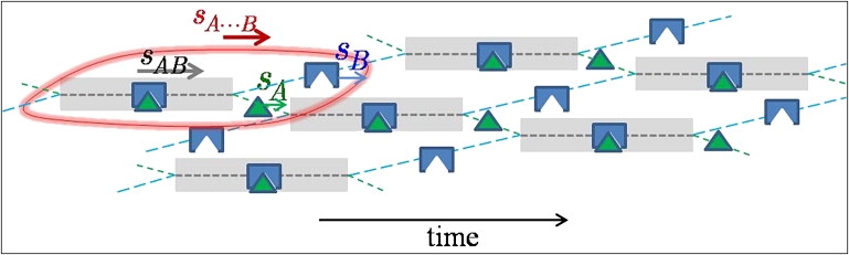
Cartoon of the effective particle A⋯B (encircled in red). Indicated is the fractional time that A (green) and B (blue) spend free or in complex (gray-shaded time intervals). The representation is faithful with regard to relative concentrations, relative velocities, and relative species lifetimes. Component A spends a smaller fraction of time free than B, resulting in a match of their time-average velocities. An animation is shown in Fig. S4 in the Supporting Material.

This picture naturally explains the occurrence of a single reaction boundary that sediments at a velocity that is neither that of free A, free B, or the complex, with molar ratio unequal to the stoichiometry of the reaction. An immediate consequence is the previously unrecognized rule that all reaction boundaries must exhibit a composition R_A⋯B less than unity, consistent with Eq. 7: Because the free state of A has a lower velocity than free B, the fractional time a molecule A spends in the free state has to be short, in order not to violate the principle that the average velocities of A and B must match.

It is instructive to compare the predictions of EPT for the average s values, boundary composition, and fractional amplitude of the undisturbed boundary with the values determined by GJT after numerical integration of the polydisperse asymptotic boundary. To this end, we comprehensively sampled the parameter space of loading concentrations {c_Atot, c_Btot} along many different trajectories (Fig. 4 and Fig. S4, Fig. S5, Fig. S6, and Fig. S7 in the Supporting Material). Overall, there is excellent qualitative agreement in describing all the hallmarks of the reacting system. Quantitatively, the agreement is close to the usual experimental precision, for the data shown in Fig. 4 exhibiting root-mean-square deviations in s_A⋯B of 0.015 S, in R_A⋯B of 2.0%, and in c_undist/c_Xtot of 5.3%. The largest deviations can be discerned where the dispersion of the GJT boundary is highest, which occurs close to the phase transition line.

Figure 4.

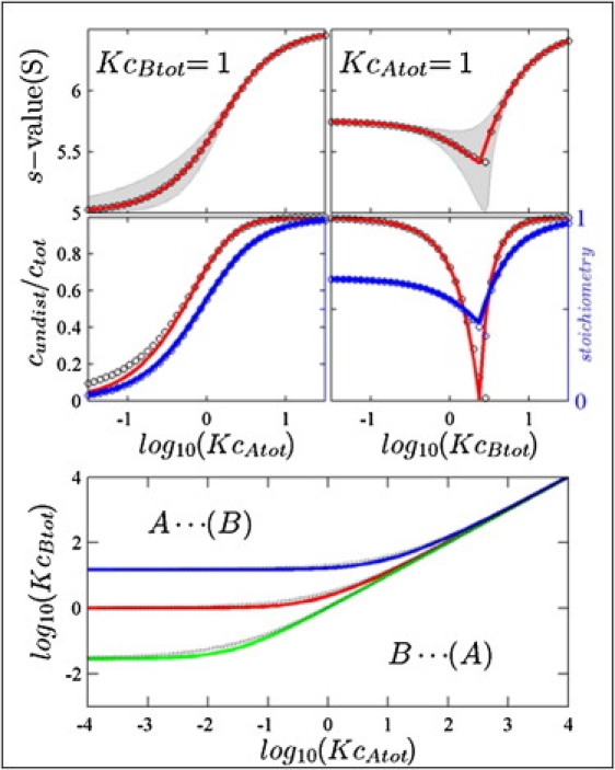
Comparison between the predictions from GJT and EPT. (Top) Weighted-average s-values from GJT by integration of the velocity distributions $d\widehat{c}/dv$ (circles) and EPT predictions for s_A⋯B (red line), along trajectories of Kc_Btot= 1 (left) or Kc_Atot= 1 (right), for the same model system as in Fig. 1. The velocity range of $d\widehat{c}/dv$ predicted by GJT as a function of concentration is indicated as the gray area. (Center) Relative amplitude of the undisturbed boundary c_undist/c_Xtot (left ordinate) as predicted from GJT (black circles) and EPT (red lines), and stoichiometry of the reaction boundary R_A⋯B (right ordinate) predicted from GJT (blue circles) and predicted by EPT (blue line). (Bottom) Phase transition line as analytically predicted from EPT (solid lines) and determined iteratively by GJT (black dotted lines), shown in red for the same system as in Fig. 1, in green for a system where the free species are similar in sedimentation coefficient (s_A = 4.9 S, s_B = 5.0 S, and s_AB = 8.5 S), and in blue for a system where A is a very small compared to B (s_A = 0.5 S, s_B = 5.0 S, and s_AB = 5.3 S).

The lower panel of Fig. 4 shows the phase transition line determined from iteratively sampling GJT (black dotted lines) and our analytical prediction (solid lines). In addition to the results for the system of Fig. 1 (red), equivalent data are presented for systems with more similar-sized binding partners (s_A ≈ s_B) in green, and more dissimilar binding partners (s_A ≪ s_B) in blue. EPT and GJT agree very well, again exhibiting the largest deviations in the region where we found the strongest polydispersity of the GJT boundary.

Next, we studied in more detail the phase transition line. Its asymmetry is remarkable. Only in the limit of concentrations high above the dissociation equilibrium constant K_D does it coincide with the equimolar line. At low concentrations of A, the transition approaches a constant value

$$c_{\text{Btot},\min }^{\ast }=K_{\text{D}}\left(s_{\text{B}}-s_{\text{A}}\right)/\left(s_{\text{AB}}-s_{\text{B}}\right).$$ (10)

For small ligands binding to large macromolecules (s_B − s_A ≫ s_AB − s_B), the critical concentration of B required for the phase transition is far above K_D, whereas for similar-sized molecules (s_A ≈ s_B) the threshold is very low. Surprisingly, at low concentration of A, even a very large molar excess of B may not be able push A entirely into the reaction boundary. The reason for this behavior can be sought in the requirement that s_A⋯B > s_B, which follows from Eqs. 5 and 6, as well as from the physical picture of Fig. 3: At low loading concentrations, the fractional population of A being ligated is not sufficiently high to elevate the time-average velocity of all A above that of free B. Therefore, A must partition into the undisturbed and the fast-moving reaction boundary, even at very low concentrations. Inspection of Eq. 7 shows that at the transition point, the stoichiometry A:B approaches zero for very low concentrations of A. This is possible, because in this limit, s_A⋯B approaches s_B, such that the relative lifetime of the free state of B can be very long.

An overview of the complete set of boundary properties for different model systems based on Eqs. 5–7 is shown in Fig. 5 (and can be produced for any parameter combinations in the public domain software SEDPHAT). They can be used as an aid in the design of SV analytical ultracentrifugation experiments. For example, determining the stoichiometry of a reaction is a frequent—and often the most important—goal of SV analytical ultracentrifugation experiments. For the system in Fig. 1, when keeping constant c_Atot = K_D at increasing concentrations of B, the phase transition of the undisturbed boundary occurs at c_Btot = 2.4 K_D. If the undisturbed boundary is misinterpreted to reflect the molar excess of the reaction, the presence of 2:1 or 3:1 complexes may be erroneously deduced. Even with c_Atot = 10 K_D, the phase transition requires c_Btot = 13.4 K_D, which would still not lead to unambiguous assessment of the correct stoichiometry. Errors grow strongly with more-dissimilar binding partners (s_B − s_A ≫ s_AB − s_B), and decrease for binding partners with similar s values.

Figure 5.

Properties of the reaction boundary A⋯B as a function of the total loading concentration of A and B, calculated by EPT for the system of Fig. 1. (Top) Velocity of the reaction boundary s_A⋯B following Eq. 6. (Center) Composition R_A⋯B of the reaction boundary following Eq. 7. (Bottom) Fractional signal of the undisturbed boundary, assuming that both components are globular with equal weight-based extinction coefficients. In all plots the line for the phase transition c_Btot^∗(c_Atot) is shown as a black dotted line, separating the region of A⋯(B) in the upper-left quadrant from B⋯(A) elsewhere.

An alternative approach to determine the complex stoichiometry is the measurement of the composition of the reaction boundary by multisignal SV. Here, it is advantageous to use high total concentrations of A in combination with moderate or low total concentrations of B. (Along lines of constant c_Atot, at higher concentration of B closer to the phase transition line, free A becomes limiting, consequently leading to lower s values and lower fractional saturation of B in the reaction boundary.) In the system of Fig. 1, for example, with c_Atot = 10 K_D, any concentration c_Btot < K_D will lead to a reaction boundary composition of ≈0.95, close to the correct stoichiometry (Fig. 5, center). Even in the limit of very small ligands, (s_AB−s_A)/(s_B−s_A) ≈ 1, the same concentration range will always lead to a boundary composition > 0.90, and this value approaches 1.0 in the limit of similar-sized A and B, when (s_AB−s_A)/(s_B−s_A) → ∞.

Discussion

The goal of this article's work was to develop a simple physical picture of comigration that occurs for rapidly reacting systems in the gravitational field. We also aimed to obtain physical insights into the relationships of concentration, sedimentation, and reaction parameters that govern the sedimentation behavior of the system, since these relationships remain obscure when relying on numerical solutions of the Lamm PDE.

We found that this can be achieved with generalized functions that can be shown to solve the same set of partial differential equations subject previously to GJT. In contrast to GJT, which describes asymptotic shapes of the reaction boundary in terms of differential velocity distributions, EPT has a different focus and only aims to describe the overall fluxes in the plateau region. This is achieved by limiting the description of the reaction boundary to the approximation with a monodisperse step-function, which can be regarded as an equivalent boundary position moving with a velocity consistent with the overall mass balance of the reaction boundary (invariant to the presence of diffusion). In this way, EPT naturally leads to the time-average sedimentation coefficients of all cosedimenting molecules in the reaction region, and the requirement that these time-average sedimentation coefficients must match. Thus, although not describing realistically the boundary shapes, EPT provides, for the first time, simple analytical expressions that describe the overall boundary pattern and phase behavior of the system. (In a forthcoming work, EPT will be applied to study the diffusive properties of reaction boundaries (P. Schuck, unpublished).)

The focus on the average composition and sedimentation velocity of the undisturbed and reaction boundary is fully adequate for the information content that can be easily extracted from experimental reaction boundaries, for example, with c(s) or other sedimentation coefficient distribution analyses. Even under experimental conditions where one can clearly detect the presence of polydispersity in broad reaction boundaries close to the phase transition point, within the typical experimental signal/noise ratio, one can reliably quantify only the average properties of the reaction boundary. (Also, it should be noted that current differential sedimentation coefficient distributions are typically extracted from experimental data representing the complete time-course of sedimentation, and therefore, as shown in (21), radial dilution at the later stage of the experiments with sector-shaped geometry has only a trivial impact on the results, justifying the application of the constant force and rectangular geometry picture of EPT.)

Conceptually, EPT can clarify features of SV analytical ultracentrifugation of interacting systems that previously remained rather mysterious, such as the mechanism of comigration of free species and complex in a single reaction boundary. It also describes previously unrecognized features of reaction boundaries, including the discovery of a phase transition line and its limiting values.

In practice, the overview of the phase behavior can be useful in the design of experiments. For example, the determination of the complex stoichiometry of a rapidly reversible interaction is an important application of SV. A common assumption is that the undisturbed boundary reflects the molar excess over the reaction stoichiometry. In this regard, the location of the phase transition line is a very important factor. For very dissimilar-sized molecules, unless very high concentrations can be used (e.g., ≫ 10 K_D(s_B−s_A)/(s_AB−s_B)), misleading transition point stoichiometries may be obtained, or, unexpectedly, no transition line may be encountered at all, irrespective of the molar ratio of loading concentrations. In contrast, EPT predicts that the alternative approach of using multisignal sedimentation velocity to probe the composition of the reaction boundary can lead to results correctly reflecting the complex stoichiometry even at moderate concentrations, without strong dependence on relative particle size. Practical examples for the application of the two approaches and their contrasting results for the stoichiometry estimates can be found in recent studies on the pyruvate dehydrogenase complex (30,31).

Similarly, the results from EPT may be used, for a given set of interacting macromolecules, to design experiments that will lead to reaction boundary velocities close to that of the complex, to facilitate hydrodynamic modeling and the comparison with translational friction coefficients of model structures (32–34). Interestingly, these conditions do not completely overlap with those leading to boundary compositions close to the reaction stoichiometry.

It is remarkable that the phase diagram of coupled migration and rapid reaction exhibits concentration-dependent features that are much sharper than typical noncooperative binding isotherms (bottom panel in Fig. 5). Where the undisturbed boundary vanishes and its constituent switches, a distinct, sharp increase in its amplitude occurs along with a discontinuous change in the s value of the undisturbed boundary. Conditions close to or at the transition points may offer unconventional experimental approaches for the determination of binding affinities at low concentrations. Further studies will show whether this concentration regime can be experimentally exploited.

EPT should also be useful for practical data analysis. It offers the opportunity for a robust analysis of systems that are experimentally not sufficiently homogeneous and/or not sufficiently information rich to permit direct fitting with the Lamm PDE of a system of interacting species. Since the PDE approach describes each species as being discrete (though interacting), one could argue that a precondition for the application of Lamm PDE modeling is that all free components, when studied individually, can be described well with a single discrete, noninteracting Lamm equation solution (e.g., that the quality of fit with c(s) distribution and with a single noninteracting species model will be equivalent). In practice, this is rarely the case due to the exquisite sensitivity of SV analytical ultracentrifugation to impurities and virtually ubiquitous degradation and aggregation products. Frequently, however, diffusion-deconvoluted sedimentation coefficient distributions still allow one to clearly discern the boundary components of the interacting system, and determine their composition, amplitudes, and s values, and the isotherms from the concentration-dependence of these quantities can be modeled with expressions from EPT. Although these isotherms can, in principle, also be modeled with solutions of GJT (as we have shown previously (19)), the application of GJT to systems with a complexity higher than two-site binding has never been attempted, to our knowledge, and seems virtually intractable. EPT, on the other hand, can readily be applied to n-site binding processes. These methods were implemented in the software SEDPHAT for isotherm analysis of experimental data.

Even though we have only developed the theory for two-component mixtures, which can exhibit, at most, two boundaries, it should be possible to apply the same principles to higher-order mixtures. For example, three-component mixtures are expected to exhibit three boundaries (one undisturbed, one two-component reaction boundary, and one three-component reaction boundary). These will likely carry correspondingly more information-rich phase behavior, potentially providing a unique avenue to gain insight into rapidly reversible multicomponent mixtures. For such systems, Lamm PDE approaches seem even more problematic than for two-component mixtures. Finally, as EPT is neither implying predictions of the detailed boundary shapes, nor of the details of transport, it may be applied equally to the quantitative study of rapidly interacting systems in highly nonideal solvents, for example, how the interaction of fluorescently labeled molecules in human serum (35,36) leads to a partitioning into undisturbed and reaction boundaries.

Supporting Material

Four figures and three movies are available at http://www.biophysj.org/biophysj/supplemental/S0006-3495(10)00152-9.

References

- 1.Gilbert G.A., Jenkins R.C. Boundary problems in the sedimentation and electrophoresis of complex systems in rapid reversible equilibrium. Nature. 1956;177:853–854. doi: 10.1038/177853a0. [DOI] [PubMed] [Google Scholar]
- 2.Gilbert G.A., Jenkins R.C. Sedimentation and electrophoresis of interacting substances. II. Asymptotic boundary shape for two substances interacting reversibly. Proc. Royal Soc. A (Lond.) 1959;253:420–437. [Google Scholar]
- 3.Winzor D.J., Scheraga H.A. Studies of chemically reacting systems on Sephadex. I. Chromatographic demonstration of the Gilbert theory. Biochemistry. 1963;2:1263–1267. doi: 10.1021/bi00906a016. [DOI] [PubMed] [Google Scholar]
- 4.Ackers G.K., Thompson T.E. Determination of stoichiometry and equilibrium constants for reversibly associating systems by molecular sieve chromatography. Proc. Natl. Acad. Sci. USA. 1965;53:342–349. doi: 10.1073/pnas.53.2.342. [DOI] [PMC free article] [PubMed] [Google Scholar]
- 5.Cann J.R. Effects of diffusion on the electrophoretic behavior of associating systems: the Gilbert-Jenkins theory revisited. Arch. Biochem. Biophys. 1985;240:489–499. doi: 10.1016/0003-9861(85)90055-4. [DOI] [PubMed] [Google Scholar]
- 6.Nichol L.W., Ogston A.G. A generalized approach to the description of interacting boundaries in migrating systems. Proc. R. Soc. Lond. B. Biol. Sci. 1965;163:343–368. [Google Scholar]
- 7.Cann J.R. Academic Press; New York: 1970. Interacting Macromolecules. [Google Scholar]
- 8.Fujita H. John Wiley & Sons; New York: 1975. Foundations of Ultracentrifugal Analysis. [Google Scholar]
- 9.Goad W.B., Cann J.R. V. Chemically interacting systems. I. Theory of sedimentation of interacting systems. Ann. N. Y. Acad. Sci. 1969;164:192–225. doi: 10.1111/j.1749-6632.1969.tb14039.x. [DOI] [PubMed] [Google Scholar]
- 10.Cox D.J. Computer simulation of sedimentation in the ultracentrifuge. IV. Velocity sedimentation of self-associating solutes. Arch. Biochem. Biophys. 1969;129:106–123. doi: 10.1016/0003-9861(69)90157-x. [DOI] [PubMed] [Google Scholar]
- 11.Claverie J.-M. Sedimentation of generalized systems of interacting particles. III. Concentration-dependent sedimentation and extension to other transport methods. Biopolymers. 1976;15:843–857. doi: 10.1002/bip.1976.360150504. [DOI] [PubMed] [Google Scholar]
- 12.Stafford W.F., Sherwood P.J. Analysis of heterologous interacting systems by sedimentation velocity: curve fitting algorithms for estimation of sedimentation coefficients, equilibrium and kinetic constants. Biophys. Chem. 2004;108:231–243. doi: 10.1016/j.bpc.2003.10.028. [DOI] [PubMed] [Google Scholar]
- 13.Dam J., Velikovsky C.A., Schuck P. Sedimentation velocity analysis of heterogeneous protein-protein interactions: Lamm equation modeling and sedimentation coefficient distributions c(s) Biophys. J. 2005;89:619–634. doi: 10.1529/biophysj.105.059568. [DOI] [PMC free article] [PubMed] [Google Scholar]
- 14.Lamm O. The differential equations of ultracentrifugation. Ark. Mat. Astr. Fys. 1929;21B:1–4. [Google Scholar]
- 15.Schuck P. Sedimentation analysis of noninteracting and self-associating solutes using numerical solutions to the Lamm equation. Biophys. J. 1998;75:1503–1512. doi: 10.1016/S0006-3495(98)74069-X. [DOI] [PMC free article] [PubMed] [Google Scholar]
- 16.Ali S.A., Iwabuchi N., Arisaka F. Reversible and fast association equilibria of a molecular chaperone, gp57A, of bacteriophage T4. Biophys. J. 2003;85:2606–2618. doi: 10.1016/s0006-3495(03)74683-9. [DOI] [PMC free article] [PubMed] [Google Scholar]
- 17.Sontag C.A., Stafford W.F., Correia J.J. A comparison of weight average and direct boundary fitting of sedimentation velocity data for indefinite polymerizing systems. Biophys. Chem. 2004;108:215–230. doi: 10.1016/j.bpc.2003.10.029. [DOI] [PubMed] [Google Scholar]
- 18.Cann J.R. Effects of microheterogeneity on sedimentation patterns of interacting proteins and the sedimentation behavior of systems involving two ligands. Methods Enzymol. 1986;130:19–35. doi: 10.1016/0076-6879(86)30005-3. [DOI] [PubMed] [Google Scholar]
- 19.Dam J., Schuck P. Sedimentation velocity analysis of heterogeneous protein-protein interactions: sedimentation coefficient distributions c(s) and asymptotic boundary profiles from Gilbert-Jenkins theory. Biophys. J. 2005;89:651–666. doi: 10.1529/biophysj.105.059584. [DOI] [PMC free article] [PubMed] [Google Scholar]
- 20.Correia J.J. Analysis of weight average sedimentation velocity data. Methods Enzymol. 2000;321:81–100. doi: 10.1016/s0076-6879(00)21188-9. [DOI] [PubMed] [Google Scholar]
- 21.Schuck P. On the analysis of protein self-association by sedimentation velocity analytical ultracentrifugation. Anal. Biochem. 2003;320:104–124. doi: 10.1016/s0003-2697(03)00289-6. [DOI] [PubMed] [Google Scholar]
- 22.Schuck P. Sedimentation velocity in the study of reversible multiprotein complexes. In: Schuck P., editor. Protein Interactions: Biophysical Approaches for the Study of Complex Reversible Systems. Springer; New York: 2007. [Google Scholar]
- 23.Schuck P. Size-distribution analysis of macromolecules by sedimentation velocity ultracentrifugation and Lamm equation modeling. Biophys. J. 2000;78:1606–1619. doi: 10.1016/S0006-3495(00)76713-0. [DOI] [PMC free article] [PubMed] [Google Scholar]
- 24.Schuck P., Perugini M.A., Schubert D. Size-distribution analysis of proteins by analytical ultracentrifugation: strategies and application to model systems. Biophys. J. 2002;82:1096–1111. doi: 10.1016/S0006-3495(02)75469-6. [DOI] [PMC free article] [PubMed] [Google Scholar]
- 25.Brown P.H., Balbo A., Schuck P. On the analysis of sedimentation velocity in the study of protein complexes. Eur. Biophys. J. 2009;38:1079–1099. doi: 10.1007/s00249-009-0514-1. [DOI] [PMC free article] [PubMed] [Google Scholar]
- 26.Balbo A., Minor K.H., Schuck P. Studying multiprotein complexes by multisignal sedimentation velocity analytical ultracentrifugation. Proc. Natl. Acad. Sci. USA. 2005;102:81–86. doi: 10.1073/pnas.0408399102. [DOI] [PMC free article] [PubMed] [Google Scholar]
- 27.Mok Y.F., Howlett G.J. Sedimentation velocity analysis of amyloid oligomers and fibrils. Methods Enzymol. 2006;413:199–217. doi: 10.1016/S0076-6879(06)13011-6. [DOI] [PubMed] [Google Scholar]
- 28.Binger K.J., Pham C.L., Howlett G.J. Apolipoprotein C-II amyloid fibrils assemble via a reversible pathway that includes fibril breaking and rejoining. J. Mol. Biol. 2008;376:1116–1129. doi: 10.1016/j.jmb.2007.12.055. [DOI] [PubMed] [Google Scholar]
- 29.Gilbert L.M., Gilbert G.A. Molecular transport of reversibly reacting systems: asymptotic boundary profiles in sedimentation, electrophoresis, and chromatography. Methods Enzymol. 1978;48:195–212. doi: 10.1016/s0076-6879(78)48011-5. [DOI] [PubMed] [Google Scholar]
- 30.Smolle M., Prior A.E., Lindsay J.G. A new level of architectural complexity in the human pyruvate dehydrogenase complex. J. Biol. Chem. 2006;281:19772–19780. doi: 10.1074/jbc.M601140200. [DOI] [PMC free article] [PubMed] [Google Scholar]
- 31.Brautigam C.A., Wynn R.M., Chuang D.T. Subunit and catalytic component stoichiometries of an in vitro reconstituted human pyruvate dehydrogenase complex. J. Biol. Chem. 2009;284:13086–13098. doi: 10.1074/jbc.M806563200. [DOI] [PMC free article] [PubMed] [Google Scholar]
- 32.García De La Torre J., Huertas M.L., Carrasco B. Calculation of hydrodynamic properties of globular proteins from their atomic-level structure. Biophys. J. 2000;78:719–730. doi: 10.1016/S0006-3495(00)76630-6. [DOI] [PMC free article] [PubMed] [Google Scholar]
- 33.Aragon S. A precise boundary element method for macromolecular transport properties. J. Comput. Chem. 2004;25:1191–1205. doi: 10.1002/jcc.20045. [DOI] [PubMed] [Google Scholar]
- 34.Rai N., Nöllmann M., Rocco M. SOMO (SOlution MOdeler) differences between x-ray- and NMR-derived bead models suggest a role for side chain flexibility in protein hydrodynamics. Structure. 2005;13:723–734. doi: 10.1016/j.str.2005.02.012. [DOI] [PubMed] [Google Scholar]
- 35.Kroe R.R., Laue T.M. NUTS and BOLTS: applications of fluorescence-detected sedimentation. Anal. Biochem. 2009;390:1–13. doi: 10.1016/j.ab.2008.11.033. [DOI] [PMC free article] [PubMed] [Google Scholar]
- 36.Demeule B., Shire S.J., Liu J. A therapeutic antibody and its antigen form different complexes in serum than in phosphate-buffered saline: a study by analytical ultracentrifugation. Anal. Biochem. 2009;388:279–287. doi: 10.1016/j.ab.2009.03.012. [DOI] [PubMed] [Google Scholar]
Associated Data
This section collects any data citations, data availability statements, or supplementary materials included in this article.