Abstract
We propose an integrated registration and clustering algorithm, called “consistency clustering”, that automatically constructs a probabilistic white-matter atlas from a set of multi-subject diffusion weighted MR images. We formulate the atlas creation as a maximum likelihood problem which the proposed method solves using a generalized Expectation Maximization (EM) framework. Additionally, the algorithm employs an outlier rejection and denoising strategy to produce sharp probabilistic maps of certain bundles of interest. We test this algorithm on synthetic and real data, and evaluate its stability against initialization. We demonstrate labeling a novel subject using the resulting spatial atlas and evaluate the accuracy of this labeling. Consistency clustering is a viable tool for completely automatic white-matter atlas construction for sub-populations and the resulting atlas is potentially useful for making diffusion measurements in a common coordinate system to identify pathology related changes or developmental trends.
Keywords: DTI, Anatomical atlas, Clustering, Segmentation, Tractography, Diffusion imaging, White matter atlas
1 Introduction
The human brain is not a single homogeneous entity, rather it consists of hundreds of distinct functional structures in the form of gray matter, and numerous connections between these structures in the form of white matter tracts. The field of neuroscience is often interested in studying the effects of neural diseases on specific structures. Some of these effects could be a change in size, shape or tissue integrity. For example, it has been reported that in the case of schizophrenia, white matter connectivity in the fornix, corpus callosum, and cingulum tracts degenerates (Kubicki et al. 2005).
These studies usually depend on manual segmentations obtained by trained experts from structural magnetic resonance (MR) images. However, structural MRI offers little or no contrast in many areas of interest, such as in deep gray matter or along white matter tracts. This is why the recent introduction of diffusion weighted imaging (DWI) as a new MRI modality has caused much excitement.
DWI is an imaging modality that measures free water diffusion, i.e. Brownian motion, of the endogenous water in tissue. This water diffusion is measured for the entire brain using directional gradients in the MRI machine. Unlike structural MRI, however, DWI does not result in a single image, but a series of images, each one quantifying the amount of water diffusion in a specific direction. These images are then combined together to calculate a 3D water diffusion probability distribution function (pdf) for every voxel. The most common way of calculating this pdf is to assume the water diffusion is Gaussian for a given voxel and fit the data from individual DWI images to this model, resulting in the diffusion tensor images (DTI) (Basser et al. 1994).
It is also possible to relax the Gaussian assumption on the diffusion pdf to describe non-Gaussian diffusion distributions. There are several methods designed for this purpose, and these include Q-space imaging (Callaghan 1993), Diffusion Spectrum Imaging (Wedeen et al. 2000) and Q-Ball imaging (Tuch 2002). These methods have the potential to provide a more complete description of the underlying tissue properties. However, high angular diffusion analysis is still an active research area and DTI remains the most commonly used method in a clinical setting.
In human brain tissue, the water diffusion is not the same in all directions, since it is obstructed by structural elements such as cell membranes or myelin. When this obstruction constrains the water diffusion in a coherent direction, such as within the cerebral white matter, the resulting water diffusion tensor becomes anisotropic, containing information about the directionality of the axon bundles (LeBihan et al. 1993; Pierpaoli and Basser 1996). Thus, quantification of water diffusion in tissue through diffusion MRI provides a unique way to look into white matter organization of the brain.
The traditional way to obtain an image segmentation is to define a similarity measure between the diffusion measurements in each voxel and then to calculate a solution that maximizes a segmentation quality measure that depends on this similarity. The most commonly used similarity measure for diffusion tensors in the literature is the Frobenius norm of the difference (Wiegell et al. 2003; Feddern et al. 2003; Rousson et al. 2004; Wang and Vemuri 2004). There are also other measures that depend on fractional anisotropy (a scalar invariant of the diffusion) (Zhukov et al. 2003), symmetrized Kullback-Leibler divergence between tensors (Wang and Vemuri 2005), normalized tensor scalar product (Jonasson et al. 2005; Jonasson et al. 2007), and angular distance between principle diffusion directions (Pfefferbaum et al. 2000; Ziyan et al. 2006; Ziyan and Westin 2008). Once a tensor similarity is chosen, the next step is to identify a quality measure and an optimizer. Different segmentation methods are proposed in the literature, including the k-means algorithm (Wiegell et al. 2003), mean-shift algorithm (Duan et al. 2007), region-based and edge-based level sets (Zhukov et al. 2003; Feddern et al. 2003; Rousson et al. 2004; Wang and Vemuri 2004; Jonasson et al. 2005). Most of these methods require a good initialization for successful segmentation. The initialization methods used were atlas-based (Wiegell et al. 2003; Jonasson et al. 2007), or manual (Zhukov et al. 2003; Feddern et al. 2003;Wang and Vemuri 2004; Lenglet et al. 2006; Wang and Vemuri 2005).
Since diffusion MRI data contains information about the directionality of the water diffusion, it is interesting to attempt to reconstruct the underlying white matter tracts. Reconstruction typically consists of starting at a voxel and following the most likely path of diffusion until a stopping criterion is reached. This sort of reconstruction is called tractography and results in a set of 3D curves, called fibers. We know that typical in-vivo imaging resolution is too low to reconstruct individual axons from the diffusion MRI data, but since these axons tend to move coherently in space, the larger white matter tracts appear as fiber bundles in tractography (Maddah et al. 2005; Maddah et al. 2007; O’Donnell and Westin 2005).
Since larger white matter tracts become evident as fiber bundles in tractography, a natural extension of tractography is to identify these bundles and assign them anatomical labels. A popular technique to assign white matter anatomy to the fiber bundles is to manually select regions of interests (ROI) that are thought to correspond to a particular anatomical white matter tract, and label all the fibers passing through this ROI with the corresponding anatomical label (Xu et al. 2002). In several studies it has been reported that using two ROIs per white matter tract results in more stable fiber bundle assignments than using only one ROI (Heiervang et al. 2006).
ROI based methods could be subject to user bias if the regions of interest are manually traced. Therefore several methods have been proposed to identify anatomically meaningful regions from the DTI data. One class of methods uses fibers generated via tractography and groups them into regions either interactively or automatically (Maddah et al. 2005;Maddah et al. 2007; O’Donnell and Westin 2005; Corouge et al. 2004; Gerig et al. 2004; Zhang and Laidlaw 2005; O’Donnell et al. 2006; Brun et al. 2004; Brun et al. 2003; Xia et al. 2005).
These automatic methods are based on well known clustering techniques, and they require a fiber similarity metric as an input. Several similarity metrics have been proposed including distance between fiber end points (Brun et al. 2003), Euclidean distance based on shape descriptors (Brun et al. 2004) and measures related to Hausdorff distance (Corouge et al. 2004; Gerig et al. 2004). Even though each of these metrics have specific advantages, mean closest point distance, which is based on the Hausdorff distance, has been widely used in DTI tractography clustering (Corouge et al. 2004; Ding et al. 2003; Gerig et al. 2004; O’Donnell et al. 2006; Zhang and Laidlaw 2005; Xia et al. 2005; O’Donnell and Westin 2007), and it was determined to be the most effective in a study where the ground truth is known (Moberts et al. 2005).
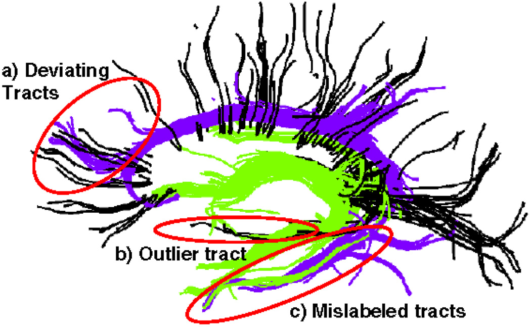
Even though resulting fiber bundles from the aforementioned clustering algorithms, in general, match well with the known anatomy, the quality of the results suffers from low SNR and low resolution of diffusion images. These issues lead to at least two types of artifacts in tractography: early termination of fibers and deviation of fibers from one bundle to another (Xu et al. 2002). (See Fig. 1 for the latter type of artifacts.)
Fig. 1.
(Color online) Some common tractography and clustering errors. Tracts from Fornix (in green) and Cingulum (in purple) bundles along with a few selected tracts from Corpus Callosum (in black) are shown as labeled using the high dimensional atlas of Sect. 3.4. The tractography noise is evident in the image as tracts deviating from one bundle to another (a) as well as a few outlier tracts (b). Also, these images contain instances where the high dimensional atlas failed to label the tracts correctly (c)
In order to reduce such errors in tractography, there have been some studies that repeat the same analysis on several individual subjects and average the results to create group maps of white matter tracts (Xu et al. 2002; Ciccarelli et al. 2003). By cross-subject averaging, the goal is to create a group map that is more robust to multiple sources of inconsistency: noise in tractography, inter-subject anatomical variability and registration errors. These methods involve single subject ROI drawing, followed by bundling of tracts that pass through these ROI’s. This yields a binary image for each bundle in each subject, that represents whether a fiber from the bundle of interest is present or not in that voxel. The next step is to employ a gray-scale image registration algorithm to co-register subjects into a common coordinate frame. This is followed by an averaging of the binary images.
In this paper we combine the group-wise registration and tract labeling with the atlas construction into an integrated and principled method. This method segments corresponding white-matter regions from a group of subjects while creating a spatial white-matter atlas of the common structures for a sub-population in a completely automatic and data-driven fashion. For this purpose, we start with a group-wise clustering to identify fiber bundles in individual subjects as well as correspondences among subjects. That is followed by a novel learning algorithm, which we call “consistency clustering”. This algorithm utilizes generalized Expectation Maximization (EM) (Mclachlan and Krishnan 2007) for optimization. Consistency clustering performs group-wise labeling, de-noising, outlier rejection, and group-wise registration in an iterative, integrated scheme and results in a spatial map that represent the most common structures in a group of subjects.
The possible uses for this algorithm are multi-fold. It could be used to compute a spatial atlas that retains only the most reproducible tracts. This atlas would represent consistently present white matter tract regions in a group of subjects. Knowing what is normal also provides a way to identify what is not, which is useful for pathology identification. Also of interest is a statistical framework for the comparison of different sub-populations, to identify disease-related or developmental changes.
2 Theory
In this section, we introduce several tools to discover the most consistent bundles across subjects and obtain a sharp atlas of these bundles. These tools include a nonlinear registration component defined on the bundles, outlier rejection and a “tract cut” operation. We formulate the problem as maximum likelihood and solve it using a generalized EM algorithm. The probabilistic framework is well-suited for extensions such as inclusion of anatomical prior information and integration with existing probabilistic atlases based on expert labeled structural MRI.
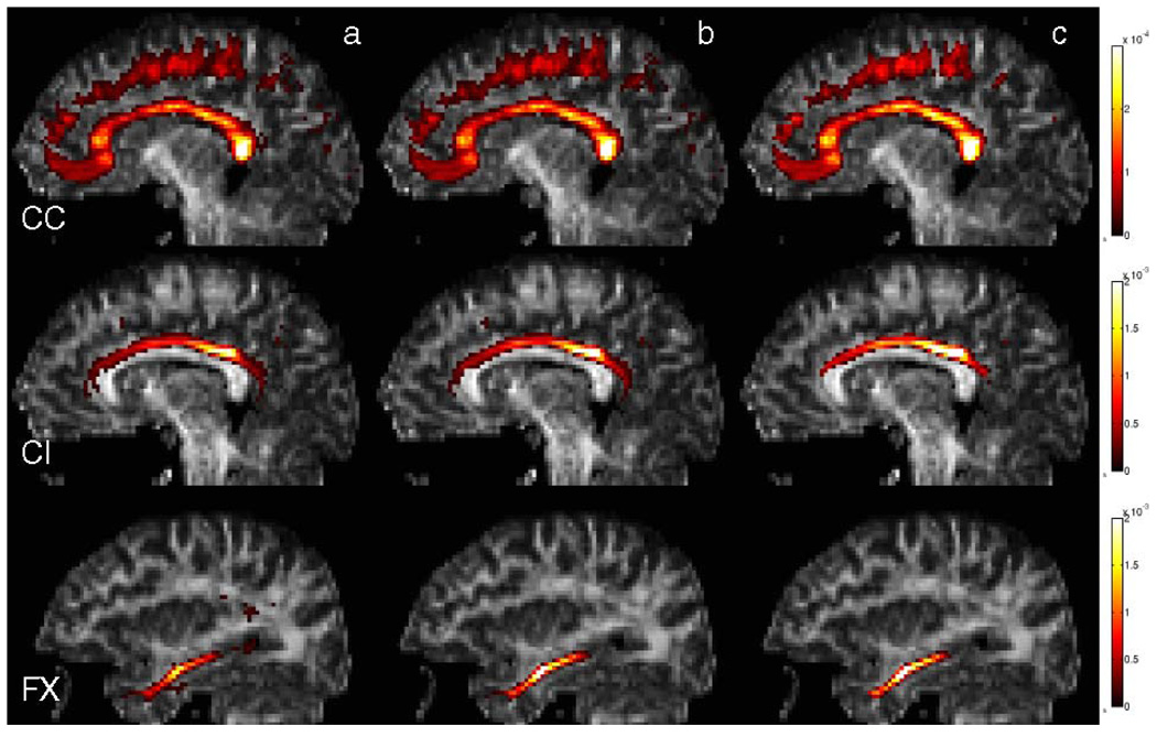
Probabilistic atlas building as described in (Xu et al. 2002) involves a sequential process of (1) registration a set of DTI images (2) labeling tracts through manually drawn ROI’s and (3) stacking the registered labels and statistical averaging, i.e. counting the number of times each voxel inherits the same label. One of the premises of such an atlas is its ability to label registered tracts. The consistency clustering algorithm we propose in this work capitalizes on this premise by iteratively relabeling tracts while building the atlas. This iterative process has the advantage of ensuring that tract labels match with the atlas that is being built and therefore results in a sharper and more consistent result (see Fig. 6(c)).
Fig. 6.
(Color online) Spatial distributions of Corpus Callosum, Cingulum and Fornix bundles from three single slices overlaid on their corresponding FA images. These maps are constructed using three different methods. (a) High-dimensional atlas, (b) consistency clustering without tract cuts, (c) consistency clustering with tract cuts. The colorbars indicate the probability of each voxel in the spatial distribution of the corresponding fiber bundle. Note that the probabilities become higher in the central regions of the bundles and the number of sporadical voxels with non-zero probabilities decrease from left to right, indicating a sharper atlas through better registration and more consistent labeling of the subjects. This observation is quantified through these distributions’ entropies in Table 1
We start with a set of subjects indexed with s ∈ {1, 2, … , S} and a set of tracts from each subject, T = {Ts} and Ts = {t ∈ Ts}. We formulate our problem as a maximum likelihood estimation of the parameter set Θ:
The term Θ includes the parameters we wish to estimate and will be defined later to include a non-parametric spatial mixture density and registration parameters. Here we assumed the tracts are statistically independent from each other in calculating L(Θ|T), the log likelihood of the data, i.e. the observed tracts. We can then derive the Expectation Maximization update equations by marginalizing this likelihood term over a set of cluster (in this context, bundle) labels c ∈ {1, 2, … , C},
for any distribution q(c), defined on the cluster labels. Now, using Jensen’s inequality:
| (1) |
| (2) |
The constant term does not depend on Θ and 𝔼q denotes expectation with respect to q. Further, the equality in (1) is met if and only if q(c) = p(c|t, Θ(n)), for a given (fixed at iteration (n)) Θ(n) (Mclachlan and Krishnan 2007). The generalized EM algorithm maximizes this lower bound using the current estimate of the parameters, Θ(n), in the E-step and re-estimates the parameters in the M-step. This iterative optimization is guaranteed to converge to a local optimum of the parameter set, Θ*. Now, let us define the probability of a tract through a non-parametric and voxelized spatial mixture density distribution:
where πc are the mixture weights and Σc πc = 1. Rs : ℝ3 ↦ ℝ3 is a subject-specific spatial transformation and Rs(t) denotes a tract obtained by applying the spatial transformation to a tract t. x ∈ ℝ3 are the samples along a given tract and ⌊x⌋ denotes quantization of x, i.e., the voxel that sample falls into. And, finally, θc(⌊x⌋) represents a non-parametric spatial distribution, quantifying the spatial probability of observing tracts from cluster c. Naturally, Σx∈X θc(x) = 1 for all c ∈ C. Then, the parameter set we wish to estimate becomes, Θ = {θc(⌊x⌋)} ∪ {πc} ∪ {Rs}.
In the next sections we will derive the specific update equations for our formulation to iteratively estimate Θ*.
2.1 E-Step
In the E-step, the algorithm updates the membership probabilities for each of the tracts given the current estimate of the parameter set Θ(n).
| (3) |
| (4) |
| (5) |
where, at every iteration (n), for all tracts t.
2.2 M-Step
In the M-step, the algorithm updates the parameter set Θ to maximize the expected value of the log likelihood. From (2), ignoring the constant term which is independent of Θ, Θ* can be computed as:
| (6) |
For a fixed parameter set Θ(n) the update equations for can be derived using Lagrange multipliers for the corresponding constraints and setting the derivative of (6) to zero. The resulting update equations are:
| (7) |
| (8) |
where denotes the number of times warped tract samples appear in voxel ⌊x⌋. The normalizing constants are computed so that .
Unlike , the registration parameters do not have an analytical solution. However, we can derive the maximum likelihood optimization function, and optimize that iteratively using a numerical scheme. Then for each subject, the registration parameters are updated as :
| (9) |
In the last equation we parameterize the registration Rs as a set of affine transformations {Rsc} for each subject s and for each cluster c, and solve for these separately. We perform this optimization using a simplex search method (Lagarias et al. 1998) to find the 9 affine parameters that correspond to translation, rotation and scaling (no shearing).
At this point we have a set of affine registration parameters , however, not a single warp field. The last step of the registration is to fuse these affine transformations to achieve a global, smooth and invertible non-linear deformation. In this study, we employed the log-Euclidean poly-affine framework (Arsigny et al. 2006) for this purpose and the details can be found in Ziyan et al. (2007).
2.3 Tract Cut
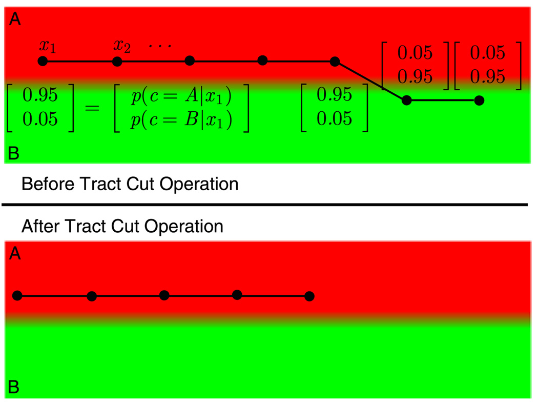
Even with the correct labeling and perfect registration, we will not be able to recover from the errors in tractography that are present as deviations of tracts from one bundle to another. One way to reduce the effects of this sort of artifacts is to remove the tract samples that do not agree with their corresponding tract labels. Our problem formulation offers a natural way to identify these deviating tract samples since it offers a maximum likelihood estimate for the label of each tract sample as well as the whole tract. The segments of every tract that consist of samples whose maximum likelihood label do not agree with the tract’s overall label are identified as deviating tract segments and can be separated from the rest of the tract, resulting in a shorter tract whose every sample has the same maximum likelihood label (see Fig. 2). More specifically, the tract cut operation removes tract samples from the tips of each tract, if the samples’ labels do not match with the tract’s overall label. The removal starts at the two ends of each tract, and continues until the label of the remaining sample at the tip of the shortened tract is no longer inconsistent with the rest of the tract.
Fig. 2.
(Color online) Illustration of the tract cut operation. The atlas contains two labels: A (in red) and B (in green). Each sample of the tract has been assigned a probability vector, p(c|xi) for c ∈ {A, B}. The overall tract label is determined as the one that maximizes the tract likelihood: p(c|t) ∝ p(c) × Πi p(xi|c). However, there are parts of this tract that does not agree with the tract’s overall label. Tract cut operation removes these parts of the tracts
2.4 Outlier Rejection
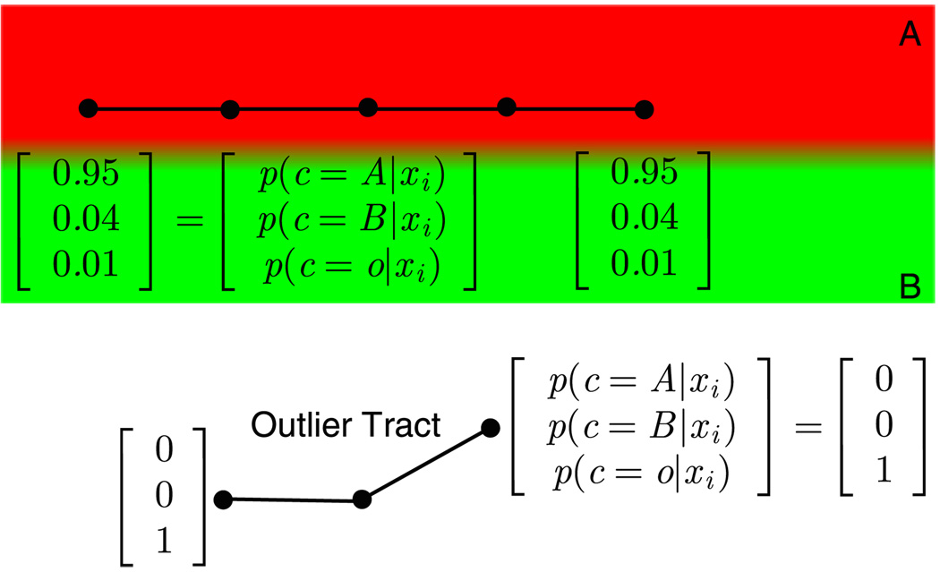
Another type of artifact is the presence of tracts that do not belong to any of the clusters. These are considered to be outlier tracts. Since these tracts are situated in the areas that are unlikely to belong to any of the clusters that are under investigation, they can be automatically identified and removed with the introduction of a default label that has a fixed very low probability throughout the image (see Fig. 3).
Fig. 3.
(Color online) Illustration of outlier removal. The atlas contains two labels: A (in red) and B (in green). A third label is created for the outliers. Each sample of the tract has been assigned a probability vector, p(c|xi) for c ∈ {A, B, o}, where ‘o’ is the label for outliers. The overall tract label is determined as the one that maximizes the tract likelihood: p(c|t) ∝ p(c) × Πi p(xi |c). If this likelihood is greater for the outlier class than any other, the tract is labeled as an outlier
3 Methods
In this section, image acquisition details and the tools used for processing the DTI data are introduced. These tools include diffusion tractography and the creation of a high dimensional atlas through spectral clustering of the tractography results.
3.1 Image Acquisition
MRI data were acquired on fifteen healthy young participants at Johns Hopkins University. The data were acquired on a 1.5 Tesla Philips Medical Systems MRI scanner using an 8-channel head coil. All participants provided informed written consent by the guidelines of the Johns Hopkins University Internal Review Board. The participants gave their informed consent in writing prior to the session.
The DTI data were acquired using a single-shot spin-echo EPI sequence. The sequence parameters were TR/TE = 7000/80 ms, b = 700 s/mm2, 5 T2 images, 30 diffusion gradient directions, 1 average, with total acquisition time 12–15 minutes. Fifty to sixty axial slices were acquired. The field-of-view was 256 × 256 mm and the matrix size was 96 × 96 to give 2.5 × 2.5 mm in-plane resolution. The slice thickness was 2.5 mm with 0 mm gap.
3.2 Tractography
Diffusion tensor imaging models microscopic diffusion in the brain tissue as a Gaussian diffusion process and encodes this information in a 3 × 3 diffusion tensor that is analogous to the covariance matrix of a 3-dimensional Gaussian random variable. The principal eigenvector of this tensor is aligned with the most likely direction of diffusion and that is the direction a streamline tractography algorithm aims to follow. In this work, tractography was performed using a Runge-Kutta order two integration of the underlying tensor field. The algorithm is initiated in every voxel in the brain with a CL value exceeding 0.25, since having a high CL value is an indicator of coherent diffusion (Westin et al. 2002). The quantity CL is defined as , where λ1, λ2, λ3 are the eigenvalues of the diffusion tensor sorted in descending order (Westin et al. 2002). Tractography is performed at a step size of 0.5 mm until the trajectory comes to the edge of the white matter, defined by a threshold of CL = 0.15.
3.3 Initial Registration
The group-wise clustering tool we employ assumes all subjects’ tractography is in a common coordinate frame, therefore a spatial normalization is needed. This normalization is performed using a group-wise, template-free affine registration algorithm (Zollei et al. 2005), known as “congealing”, on the Fractional Anisotropy (FA) images generated for each subject. This initial normalization aims to remove gross differences across subjects due to global head size and orientation. It is thus limited to a 9 parameter affine transformation that accounts for scaling, rotation and translation. The resulting transformations are then applied to each of the computed fibers to map them into a common coordinate frame for clustering. Since the fibers are represented by a set of points in 3D, the application of the computed transformation does not require interpolation, as it would in gray-scale image registration. Instead, applying the transformation is performed through a simple linear operation and does not result in blurring of fibers, which is a common artifact in gray-scale image registration.
3.4 Fiber Clustering for a High-Dimensional Atlas
Fiber clustering is based on the assumption that fibers that are in the same bundle follow a similar trajectory within the tissue. To quantify this similarity, the employed algorithm uses the mean closest point distance (Corouge et al. 2004). This is defined as the average distance from each point in one tract to its nearest distance to the other tract. This distance is then symmetrized by taking the minimum of the two distances between every fiber pair. The algorithm converts this distance into an affinity measure using a Gaussian kernel. Once these affinities are calculated for every tract pair, we employed spectral clustering with normalized cuts criteria (Shi and Malik 2000) to compute clusters of fibers.
Once clustering is completed, an expert needs to assign anatomical labels to these clusters. This is done interactively on one of the subjects by selecting clusters one by one and assigning them anatomical labels. Since the clustering is done on a number of subjects jointly, these labels are automatically transferred to all the subjects used for the clustering stage.
By clustering fibers from multiple subjects into bundles, common white matter structures are discovered in an automatic way, and the bundle models are saved with expert anatomical labels to form a high dimensional atlas (O’Donnell and Westin 2006). This atlas is called high dimensional since the clustering is done in a high dimensional space and the cluster definitions as well as the anatomical labels are saved in this high dimensional space. Even though resulting fiber bundles from labeling with such an atlas in general match well with the known anatomy, the quality of the results exhibit artifacts such as mislabeled tracts and outlier tracts labeled as with one of the anatomical labels (see Fig. 1). Also the quality of the spatial atlas obtained by simply voxelizing a set of multi-subject images labeled with a high dimensional atlas is limited (see Fig. 6(a)), which indicates that automatic identification of consistent bundles and their localization in the common coordinate frame is problematic due to limited inter-subject alignment, cross-subject anatomical variability and tractography noise.
In the current work, we utilize the automatically segmented tractography results obtained through the aforementioned semi-supervised, high-dimensional atlas framework as initial but noisy tract labels, and perform a group-wise labeling, de-noising, outlier rejection, and registration in an iterative and integrated scheme while building a spatial atlas that represent the most common structures.
4 Experiments
In this section we demonstrate the dual purposes of the consistency clustering algorithm: A group-wise clustering algorithm, as well as a robust atlas building algorithm. We apply the algorithm on synthetic data and in-vivo DTI data.
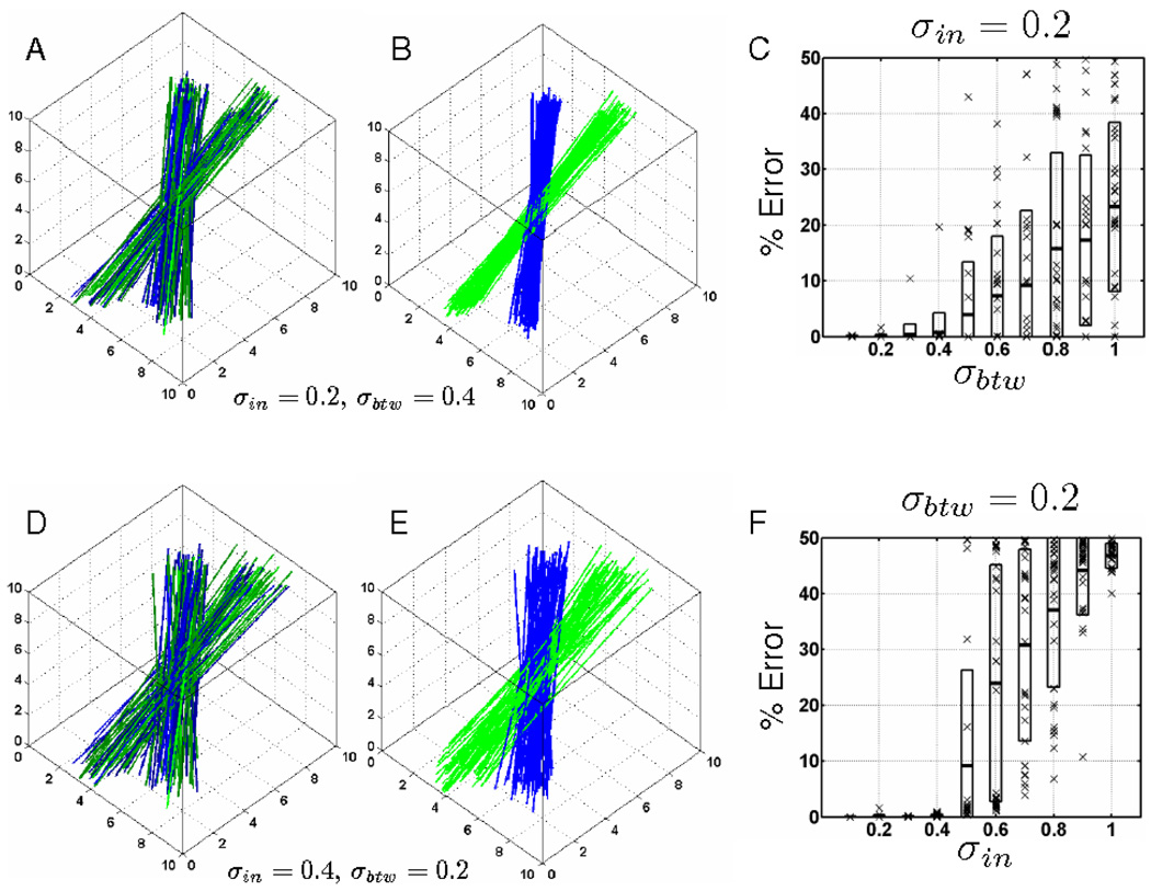
Synthetic data is created to simulate 5 subjects with two fiber bundles in each subject. The fiber bundles are crossing each other in the middle of the data range at a 30 degree angle (see Fig. 4) (when the noise parameters are set to zero). There are also two noise parameters, σin and σbtw that control the variability of the 3D lines that make up each one of these bundles. σin controls the variability within a subjects bundles and σbtw controls the variability in between two subjects bundles as described in the following: For a given starting point xst and a norm-one slope vector si for i = 1, 2—one for each bundle, each subject k is assigned a random starting point , and a random slope vector , where N(0, σ) is a zero-mean 3-dimensional random variable with a diagonal convariance matrix with diagonal elements set to σ. Once each subject’s starting point and slope is determined, each tract within the subject is generated by randomly perturbing these values to . Each line then consist of a set of uniformly spaced points in 3D, generated using these parameters. The lines are constrained to be within a pre-determined range to limit the length.
Fig. 4.
Consistency clustering results from a synthetic dataset. Each dataset consists of 5 simulated subjects with two fiber bundles crossing each other at a 30 degree angle. σin controls the variability of lines within each subject and σbtw controls the variability of lines between the subjects (see Sect. 4 for details). Figures A and D show simulated fibers from 5 subjects overlaid on top of each other and colored according to the initial random labels. Figures B and E show the same datasets as in figures A and D respectively, with the labels and registration parameters resulting from the consistency clustering algorithm. Figures C and F show the algorithm’s accuracy in labeling fibers under varying noise levels. The data is randomly created and clustered with random initialization for 30 times at each noise level increment. The cross marks represent observed error levels from each one of these experiments, and the boxes indicate one standard deviation from the mean error at each noise level increment. Figure C shows at least one correctly labeled instance at each noise level between the subjects whereas the algorithm starts to fail regularly with increasing noise within the same subject as shown in figure F
4.1 Consistency Clustering: a Clustering Algorithm
Consistency clustering is an atlas-based group-wise clustering algorithm. To demonstrate its use as a clustering algorithm we utilized synthetic data, for which we have the ground truth. To understand the effect of noise on the consistency clustering algorithm, we created synthetic data with varying noise levels. Each synthetic data set consisted of 5 subjects with two fiber bundles for each subject. We initialized the consistency clustering algorithm with random labels as in Fig. 4 (A and B) and repeated the experiment at each noise level for 30 times. The algorithm recovered the ground truth labels with high accuracy for a wide range of noise parameters as presented in Fig. 4 (C and F).
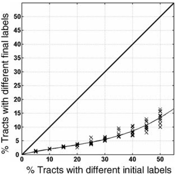
Unlike synthetic data, real DTI data does not offer ground truth to evaluate our algorithm against. However, we can still evaluate the stability of our algorithm for initialization. For this purpose, we applied the consistency clustering algorithm to 15 subjects without the outlier rejection and the tract cuts (since removing tracts and tract segments complicate the error measurement). Once the algorithm converges on an optimal set of tract labels, we stored these optimal labels to test the stability of our algorithm. A stable algorithm is expected to converge back to the same optimal labels from a range of differing initializations. To evaluate this kind of stability, we randomly changed a certain percentage of the optimal labels (varying between 5% and 50%), and rerun the algorithm initialized with these sub-optimal labels. We repeated this experiment 10 times for each percentage level, which is varied in increments of 5%. The results from these experiments are presented in Fig. 5. For a wide range corruption levels, the algorithm produced nearly identical labels as the initial optimal solution.
Fig. 5.
Stability of labels produced by consistency clustering for the 15 subject DTI data. A set of optimal labels is acquired by running the algorithm on 15 subjects’ DTI data from Fornix, Cingulum and Corpus Callosum bundles until convergence. To test for stability of these optimal labels, a certain percentage of the optimal labels (varying between 5% and 50%) are changed randomly, resulting in sub-optimal labels. These sub-optimal labels are then used as an initialization for the algorithm, to test whether the algorithm would converge back to the same optimal labels. The graph depicts the percentage errors of the tract labels at initialization (x-axis) and convergence (y-axis) stages of the algorithm. Errors are calculated as the percentage of tracts with non-optimal labels at the corresponding stage. Each cross mark indicates the error from one experiment in which a certain percentage of the optimal labels are changed and the algorithm is rerun with these corrupted labels as initialization. Solid line is produced by fitting a second degree polynomial to these experimental results. Note that varying the initial labels by 30% results in only 5% difference in the final labels
4.2 Consistency Clustering: an Atlas-building Algorithm
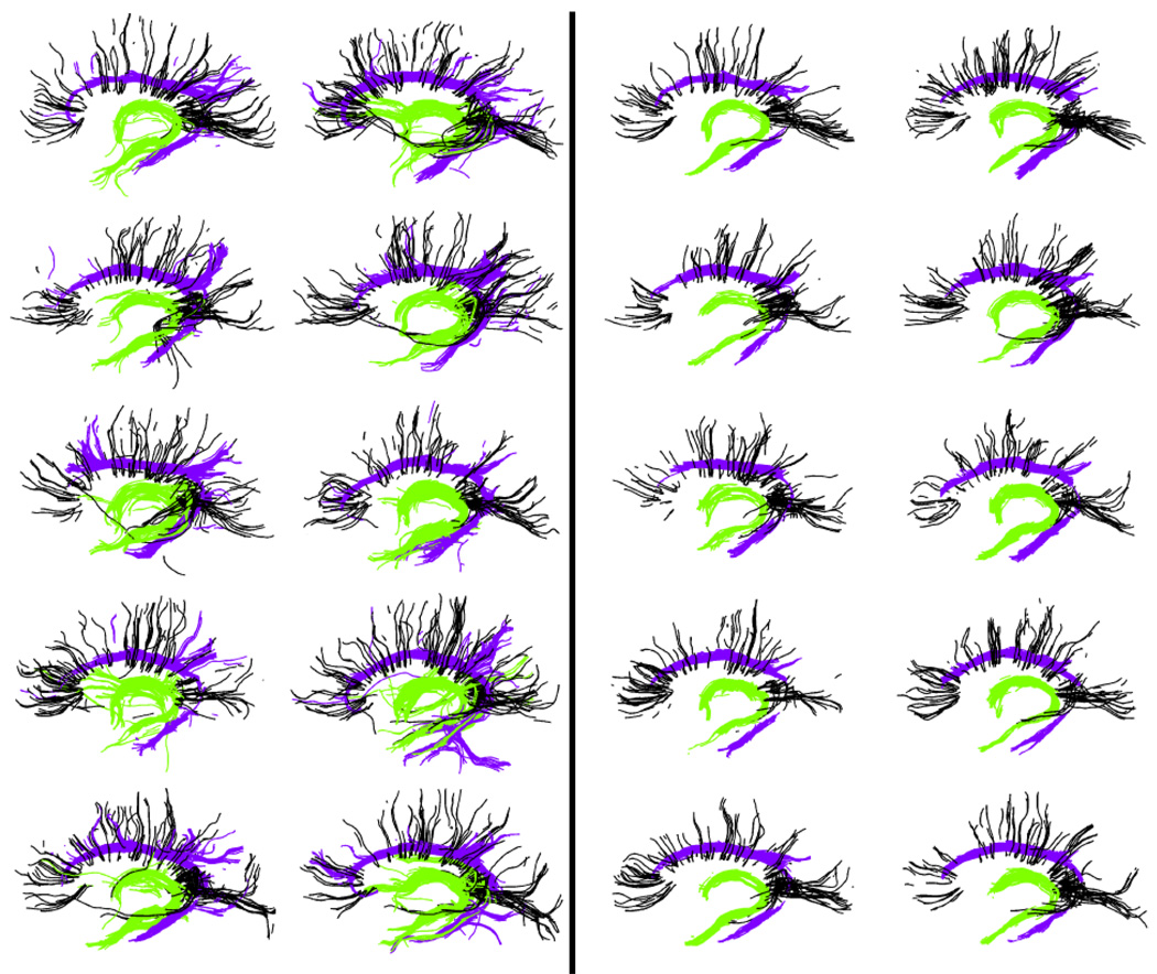
As mentioned earlier, consistency clustering is an atlas-based group-wise clustering algorithm and can also be used for creation of probabilistic MRI atlases based on DTI tractography clustering. Corpus Callosum, Cingulum and the Fornix were selected for investigation in this study, because of the specific challenges they present. These three structures are in close proximity with each other, and that results in many mislabeled fibers when labeled using a high dimensional atlas (see Fig. 7 (left)). Their close proximity also results in a number of trajectories deviating from one structure to another. These are precisely the sorts of artifacts we wish to reduce through learning common spatial distributions of fiber bundles from a group of subjects.
Fig. 7.
(Color online) Tracts from Fornix (in green) and Cingulum (in purple) bundles along with a few selected tracts from Corpus Callosum (in black) as labeled through the high-dimensional atlas (left) and through the consistency clustering with tract cuts (right). The tractography noise is evident in the images on the left as tracts deviating from one bundle to another. Also, these images contain instances where the high-dimensional atlas failed to label the tracts correctly. Consistency clustering is able identify consistent tract bundles across subjects, while tract cuts operation remove the inconsistent parts of these bundles, resulting in “core” bundles
We constructed three different atlases to compare the effects of labeling algorithms on the quality of resulting group maps. The first one is constructed using the initial labels from the high dimensional atlas. A second one is built using the consistency clustering algorithm without the outlier rejection and the tract cut operations, and the last one is generated through the consistency clustering algorithm with the outlier rejection and tract cut operations.
Tracts labeled with the high dimensional atlas qualitatively conformed with the known anatomy of the white matter; however most subjects contained individual tracts deviating from one bundle to another (Fig. 7 (left)). Also, the high dimensional atlas failed to label some of the tracts correctly, potentially due to registration errors. The proposed algorithm; however, was able to remove the segments of the tract bundles that were not consistent from subject to subject (Fig. 7 (right)).
4.3 Atlas Quality
Once the atlases are built, it is of interest to quantify the quality of these atlases. We do so through entropy, which is an information theoretic measure of uncertainty in a probability distribution. A smaller entropy measure indicates a sharper atlas, which is due to increasing similarity in the shapes of the bundles that are used to construct that atlas. These relative similarities result from a better registration or more consistent labeling across subjects. The entropy of a spatial distribution of a specific fiber bundle in our atlas notation is defined as:
Removing inconsistencies between subjects before averaging resulted in a qualitatively sharper atlas, which is presented in Fig. 6. The colored overlays indicate the probability of a tract bundle being present in any location in the brain. A whiter color indicates regions where there were more consistent alignment in the labeled tracts among the subjects, resulting in higher probability values. Spatial probabilities were greatest in the central regions of the bundles under investigation in all three atlases. However, these probabilities increase in the central regions and decrease in the perimeters with improved registration and corrected labels through the proposed algorithms. This resulting improvement in the atlas quality is quantified in Table 1 through the distribution entropies. This analysis indicates that smaller structures benefit more from the better registration and label correction the consistency clustering algorithm provides.
Table 1.
Spatial probability distribution entropies (measured in nats) for each of the structures constructed through three different methods. FX, CC and CI stands for Fornix, Corpus Callosum, and Cingulum bundles, respectively. A lower entropy value for the same bundle indicates a sharper distribution that is less contaminated with artifacts. Smaller structures seem to benefit more from the better registration and label correction the consistency clustering provides
| Method | FX | CC | CI |
|---|---|---|---|
| High dim. atlas | 8.0791 | 9.6492 | 8.1250 |
| Consistency clustering w/o cuts | 7.1830 | 9.5204 | 7.6818 |
| Consistency clustering with cuts | 6.8434 | 9.1506 | 7.0911 |
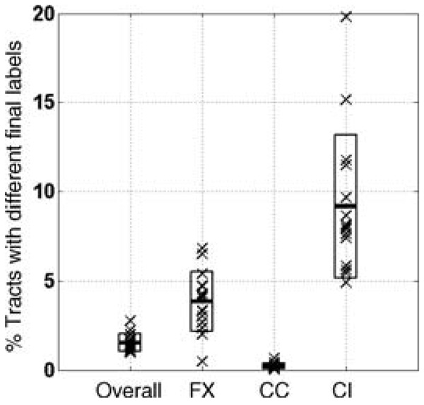
Another way of quantifying the atlas quality is through its accuracy in labeling novel subjects that were not used to build the atlas. Once again since we do not have the ground truth for the DTI tracts, we run our consistency clustering algorithm on all 15 subjects without the outlier rejection and the tract cuts and stored the resulting tract labels for later evaluation. Then we repeated this atlas building experiment 15 times, each time with 14 subjects participating in the atlas building stage. Once such an atlas is constructed, the remaining subject is labeled using the atlas through a modified EM loop that involves the registration step and the E-step until convergence. Once each one of the subjects are labeled this way, the resulting labels are then compared against the labels produced when all 15 subjects were used for the atlas construction. The overall differences in the labels were in the range of 1.0% to 2.8%. That translates to more than 97% of the labels being the same whether a subject was used in the atlas construction or not. The results from these experiments are presented in Fig. 8 for each one of three structures used in the atlas building as well as the overall results.
Fig. 8.
Evaluating the consistency of atlas-based labeling. Each cross mark represents an experiment in which one subject labeled with the atlas constructed from the remaining 14 subjects. These labels are compared against the labels produced by the atlas building algorithm with all 15 subjects included. The boxes indicate one standard deviation above and below the mean difference level. Leftmost column shows the overall differences, summarizing the results for the whole atlas, and the other three columns shows the differences for each of the structures represented in the atlas. These structures are Fornix (FX), Corpus Callosum (CC) and Cingulum (CI)
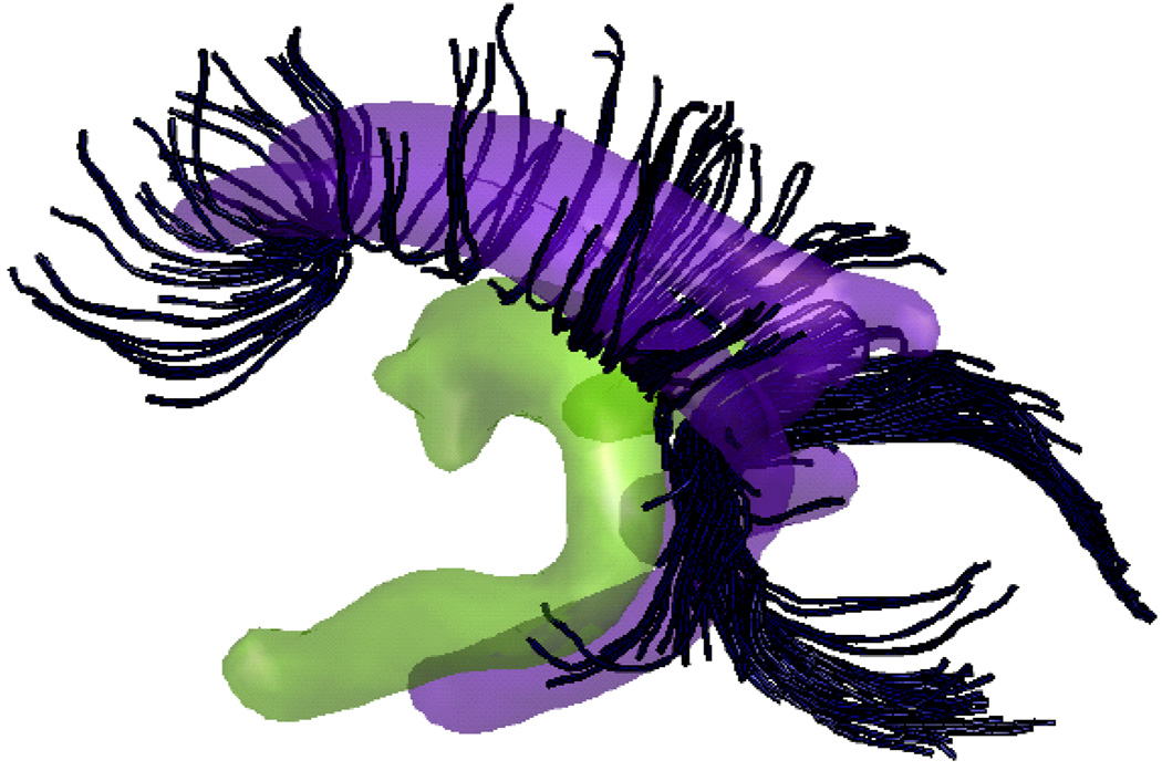
The resulting atlas from consistency clustering is also presented as isoprobability surfaces to qualitatively inspect the resulting distributions in 3D (Fig. 9). These spatial distributions retained very little of the tractography noise that was apparent in the individuals’ tract bundles, and conformed well with the known anatomy.
Fig. 9.
(Color online) Isoprobability surfaces of the spatial distributions of Fornix (in green) and Cingulum (in purple) bundles constructed from 15 subjects using the consistency clustering algorithm with tract cut operations. The surface is generated by thresholding the spatial atlas at a probability level of 10−4. A few selected tracts from Corpus Callosum (in black) are also drawn to highlight the spatial proximity of the three bundles. These spatial distributions retain very little of the tractography noise that is apparent in the individuals’ tract bundles
5 Conclusion and Discussion
In this paper, we introduced an integrated registration and clustering algorithm to segment and label fibers while computing an atlas of fiber-bundles from a set of multi-subject diffusion weighted MR images. To demonstrate the use of this algorithm, we constructed spatial distributions of three fiber bundles in close proximity. The relative closeness of these bundles causes erroneous labeling of tracts when automatically labeled with a high-dimensional atlas. However, the integrated approach we present in this paper is able to recover from these errors, resulting in a sharper atlas that is less contaminated with the mentioned artifacts.
We also demonstrated the stability of our algorithm by randomly changing the initial labels of varying proportion of the tracts. The results indicate that the solution of consistency clustering is stable under initialization and therefore is well suited for medical applications.
Another important aspect of any atlas is its ability to label novel subjects. We demonstrated that the tract labels are very similar whether a subject is used in the atlas building stage, or is left out at that stage and labeled afterward with the resulting atlas.
Furthermore, we presented a fully automated atlas construction pipeline, that consists of tractography, labeling with a high dimensional atlas and group-wise correction of the labels and registrations. With the introduction of a principled outlier rejection and tract cut scheme, we showed that it is also possible to retain only the “core” tract bundles, the tract segments that have their counterparts present in the group of subjects that is being analyzed. Since all of the fiber bundles are also aligned in a common coordinate system, it is then possible to define measurement axes, which are not limited to simple curves, for each of the core bundles and collect quantitative measurements for group-wise morphometry. This could prove to be a powerful statistical framework for the comparison of different sub-populations, to identify disease-related or developmental changes in the white matter anatomy.
In this work we used the streamline tractography since it is commonly used in the field. However, due to the low SNR and ambiguity of the tensor model in the fiber crossings, streamline tractography results in many errors. We have introduced a tract cut operation to identify and reduce these artifacts. It is of future interest, however, to include the tractography into this iterative framework to make these corrections in a more integrated way. Furthermore, since the model we introduce in this paper does not consider the source of tractography, it is suitable for use with other tractography methods. This in return provides a tool to compare different tractography algorithms by building an atlas for the population and quantifying consistency of several tractrography algorithms in different individuals. The underlying probabilistic method can also be extended for use with stochastic tractography by including resulting probabilistic information at the voxel level into the atlas.
The probabilistic nature of our algorithm makes it possible for extensions of this work and the fact that we are using spatial and voxelized atlases makes it possible to fuse diffusion MRI based white-matter atlases with ones that were created using expert labeled structural MR images.
Fig. 10.
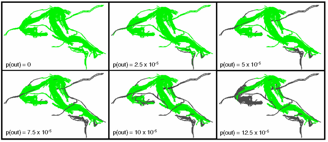
(Color online) Impact of varying outlier class probability level demonstrated on a Fornix of one exemplar subject. As the outlier class probability is increased, a larger percentage of the tracts from the Fornix (in green) are classified as outliers (in gray)
Acknowledgements
This work was supported by NIH NIBIB NAMIC U54-EB005149, NIH NCRR NAC P41-RR13218, R01- MH074794, NIH 1-R01-NS051826-01, NIH U41 RR019703 and the Athinoula A. Martinos Foundation. We are grateful to Susumu Mori at JHU for the diffusion MRI data (R01-AG20012 / P41-RR15241).
Contributor Information
Ulas Ziyan, Email: ulas@csail.mit.edu, Computer Science and Artificial Intelligence Lab, MIT, Cambridge, MA, USA.
Mert R. Sabuncu, Email: msabuncu@csail.mit.edu, Computer Science and Artificial Intelligence Lab, MIT, Cambridge, MA, USA.
W. Eric L. Grimson, Email: welg@csail.mit.edu, Computer Science and Artificial Intelligence Lab, MIT, Cambridge, MA, USA.
Carl-Fredrik Westin, Email: westin@bwh.harvard.edu, Computer Science and Artificial Intelligence Lab, MIT, Cambridge, MA, USA; Laboratory of Mathematics in Imaging, Brigham and Women’s Hospital, Harvard Medical School, Boston, MA, USA.
References
- Arsigny V, Commowick O, Pennec X, Ayache N. A fast and Log-Euclidean polyaffine framework for locally affine registration. Research report RR-5865, INRIA Sophia-Antipolis. 2006 March
- Basser PJ, Mattiello J, Le Bihan D. MR diffusion tensor spectroscopy and imaging. Biophysics Journal. 1994;66:259–267. doi: 10.1016/S0006-3495(94)80775-1. [DOI] [PMC free article] [PubMed] [Google Scholar]
- Brun A, Park H-J, Knutsson H, Westin C-F. Coloring of DT-MRI fiber traces using Laplacian eigenmaps; International conference on computer aided systems theory; 2003. pp. 564–572. [Google Scholar]
- Brun A, Knutsson H, Park H-J, Shenton ME, Westin C-F. Clustering fiber traces using normalized cuts. Medical image computing and computer assisted intervention. 2004:368–375. doi: 10.1007/b100265. [DOI] [PMC free article] [PubMed] [Google Scholar]
- Callaghan PT. Principles of nuclear magnetic resonance microscopy. Oxford: Oxford University Press; 1993. [Google Scholar]
- Ciccarelli O, Toosy AT, Parker GJM, Wheeler O, King-shott CAM, Barker GJ, Miller DH, Thompson AJ. Diffusion tractography based group mapping of major white-matter pathways in the human brain. Neuroimage. 2003;19(4):1545–1555. doi: 10.1016/s1053-8119(03)00190-3. [DOI] [PubMed] [Google Scholar]
- Corouge I, Gouttard S, Gerig G. Towards a shape model of white matter fiber bundles using diffusion tensor MRI. IEEE international symposium on biomedical imaging. 2004:344–347. [Google Scholar]
- Ding Z, Gore JC, Anderson AW. Classification and quantification of neuronal fiber pathways using diffusion tensor MRI. Magnetic Resonance in Medicine. 2003;49:716–721. doi: 10.1002/mrm.10415. [DOI] [PubMed] [Google Scholar]
- Duan Y, Li X, Xi Y. Thalamus segmentation from diffusion tensor magnetic resonance imaging. Journal of Biomedical Imaging. 2007;2 doi: 10.1155/2007/90216. [DOI] [PMC free article] [PubMed] [Google Scholar]
- Feddern C, Weickert J, Burgeth B. Level-set methods for tensor-valued images. Proceedings of the second IEEE workshop on geometric and level set methods in computer vision. 2003:65–72. [Google Scholar]
- Gerig G, Gouttard S, Corouge I. Analysis of brain white matter via fiber tract modeling. IEEE Engineering in Medicine and Biology Society. 2004;426 doi: 10.1109/IEMBS.2004.1404229. [DOI] [PubMed] [Google Scholar]
- Heiervang E, Behrens TE, Mackay CE, Robson MD, Johansen-Berg H. Between session reproducibility and between subject variability of diffusion MR and tractography measures. Neuroimage. 2006;33:867–877. doi: 10.1016/j.neuroimage.2006.07.037. [DOI] [PubMed] [Google Scholar]
- Jonasson L, Bresson X, Hagmann P, Cuisenaire O, Meuli R, Thiran J-P. White matter fiber tract segmentation in DTMRI using geometric flows. Medical Image Analysis. 2005;9:223–236. doi: 10.1016/j.media.2004.07.004. [DOI] [PubMed] [Google Scholar]
- Jonasson L, Hagmann P, Pollo C, Bresson X, Wilson CR, Meuli R, Thiran J-P. A level set method for segmentation of the thalamus and its nuclei in DT-MRI. Signal Processing. 2007;87(2):309–321. [Google Scholar]
- Kubicki M, Park H-J, Westin C-F, Nestor P, Mulkern R, Maier SE, Niznikiewicz M, Connor E, Levitt J, Frumin M, Kikinis R, Jolesz FA, McCarley R, Shenton ME. DTI and MTR abnormalities in schizophrenia: analysis of white matter integrity. Neuroimage. 2005;26:1109–1118. doi: 10.1016/j.neuroimage.2005.03.026. [DOI] [PMC free article] [PubMed] [Google Scholar]
- Lagarias JC, Reeds JA, Wright MH, Wright PE. Convergence properties of the Nelder-Mead simplex method in low dimensions. SIAM Journal of Optimization. 1998;9:112–147. [Google Scholar]
- LeBihan D, Turner R, Douek P An echo-planar NMR imaging study. Neuroreport. Vol. 4. 1993. Is water diffusion restricted in human brain white matter? pp. 887–890. [DOI] [PubMed] [Google Scholar]
- Lenglet C, Rousson M, Deriche R. DTI segmentation by statistical surface evolution. IEEE Transactions in Medical Imaging. 2006;25:685–700. doi: 10.1109/tmi.2006.873299. [DOI] [PubMed] [Google Scholar]
- Maddah M, Mewes A, Haker S, Grimson WEL, Warfield S. Automated atlas-based clustering of white matter fiber tracts from DTMRI. Medical image computing and computer assisted intervention. 2005:188–195. doi: 10.1007/11566465_24. [DOI] [PubMed] [Google Scholar]
- Maddah M, Wells WM, Warfield SK, Westin C-F, Grimson WEL. Probabilistic clustering and quantitative analysis of white matter fiber tracts. Information processing in medical imaging. 2007 doi: 10.1007/978-3-540-73273-0_31. [DOI] [PMC free article] [PubMed] [Google Scholar]
- Mclachlan GJ, Krishnan T. The EM algorithm and extensions. New York: Wiley-Interscience; 2007. [Google Scholar]
- Moberts B, Vilanova A, vanWijk JJ. Evaluation of fiber clustering methods for diffusion tensor imaging; IEEE visualization conference; 2005. pp. 65–72. [Google Scholar]
- O’Donnell L, Westin C-F. White matter tract clustering and correspondence in populations. Medical image computing and computer assisted intervention. 2005:140–147. [PubMed] [Google Scholar]
- O’Donnell L, Westin C-F. High-dimensional white matter atlas generation and group analysis. Medical image computing and computer assisted intervention (2) 2006:243–251. [PubMed] [Google Scholar]
- O’Donnell LJ, Westin C-F. Automatic tractography segmentation using a high-dimensional white matter atlas. IEEE Transactions on Medical Imaging. 2007;26(11):1562–1575. doi: 10.1109/TMI.2007.906785. [DOI] [PubMed] [Google Scholar]
- O’Donnell L, Kubicki M, Shenton ME, Grimson WEL, Westin C-F. A method for clustering white matter fiber tracts. American Journal of Neuroradiology. 2006;27(5):1032–1036. [PMC free article] [PubMed] [Google Scholar]
- Pfefferbaum A, Sullivan EV, Hedehus M, Lim KO, Adalsteinsson E, Moseley M. Age-related decline in brain white matter anisotropy measured with spatially corrected echo-planar diffusion tensor imaging. Magnetic Resonance in Medicine. 2000;44:259–268. doi: 10.1002/1522-2594(200008)44:2<259::aid-mrm13>3.0.co;2-6. [DOI] [PubMed] [Google Scholar]
- Pierpaoli C, Basser PJ. Toward a quantitative assessment of diffusion anisotropy. Magnetic Resonance in Medicine. 1996;36:893–906. doi: 10.1002/mrm.1910360612. [DOI] [PubMed] [Google Scholar]
- Rousson M, Lenglet C, Deriche R. Level set and region based surface propagation for diffusion tensor MRI segmentation. Mathematical methods in biomedical image analysis. 2004 [Google Scholar]
- Shi J, Malik J. Normalized cuts and image segmentation. IEEE Transactions in Pattern Analysis and Machine Intelligence. 2000;22(8):888–905. [Google Scholar]
- Tuch DS. Ph.D. thesis. MIT; 2002. Diffusion MRI of complex tissue structure. [Google Scholar]
- Wang Z, Vemuri BC. Tensor field segmentation using region based active contour model. European conference on computer vision. 2004:304–315. [Google Scholar]
- Wang Z, Vemuri BC. DTI segmentation using an information theoretic tensor dissimilarity measure. IEEE Transactions on Medical Imaging. 2005;24:1267–1277. doi: 10.1109/TMI.2005.854516. [DOI] [PubMed] [Google Scholar]
- Wedeen V, Reese T, Tuch D, Wiegel M, Dou J-G, Weiskoff R, Chessler D. Mapping fiber orientation spectra in cerebral white matter with Fourier transformdiffusion MRI. The International Society for Magnetic Resonance in Medicine. 2000:82. [Google Scholar]
- Westin C-F, Maier SE, Mamata H, Nabavi A, Jolesz FA, Kikinis R. Processing and visualization of diffusion tensor MRI. Medical Image Analysis. 2002;6(2):93–108. doi: 10.1016/s1361-8415(02)00053-1. [DOI] [PubMed] [Google Scholar]
- Wiegell MR, Tuch DS, Larson HWB, Wedeen VJ. Automatic segmentation of thalamic nuclei from diffusion tensor magnetic resonance imaging. Neuroimage. 2003;19:391–402. doi: 10.1016/s1053-8119(03)00044-2. [DOI] [PubMed] [Google Scholar]
- Xia Y, Turken U, Whitfield-Gabrieli SL, Gabrieli JD. Knowledge-based classification of neuronal fibers in entire brain. Medical image computing and computer assisted intervention. 2005:205–212. doi: 10.1007/11566465_26. [DOI] [PubMed] [Google Scholar]
- Xu D, Mori S, Solaiyappan M, van Zijl PCM, Davatzikos C. A framework for callosal fiber distribution analysis. Neuroimage. 2002;17:1131–1143. doi: 10.1006/nimg.2002.1285. [DOI] [PubMed] [Google Scholar]
- Zhang S, Laidlaw DH. DTI fiber clustering and cross-subject cluster analysis. The International Society for Magnetic Resonance in Medicine. 2005 [Google Scholar]
- Zhukov L, Museth K, Breen D, Whitakert R, Barr AH. Level set modeling and segmentation of DT-MRI brain data. Journal of Electronic Imaging. 2003;12:125–133. [Google Scholar]
- Ziyan U, Westin C-F. Joint segmentation of thalamic nuclei from a population of diffusion tensor MR images. Medical image computing and computer assisted intervention. 2008:279–286. doi: 10.1007/978-3-540-85988-8_34. [DOI] [PMC free article] [PubMed] [Google Scholar]
- Ziyan U, Tuch D, Westin C-F. Segmentation of thalamic nuclei from DTI using spectral clustering. Medical image computing and computer assisted intervention. 2006:807–814. doi: 10.1007/11866763_99. [DOI] [PubMed] [Google Scholar]
- Ziyan U, Sabuncu MR, O’Donnell LJ, Westin C-F. Nonlinear registration of diffusion MR images based on fiber bundles. Medical image computing and computer assisted intervention. 2007:351–358. doi: 10.1007/978-3-540-75757-3_43. [DOI] [PubMed] [Google Scholar]
- Zollei L, Learned-Miller E, Grimson WEL, Wells WM., III Efficient population registration of 3D data. International conference on computer vision for biomedical image applications. 2005 [Google Scholar]


