Multi-scale modeling in cell biology

Abstract

Biomedical research frequently involves performing experiments and developing hypotheses that link different scales of biological systems such as, for instance, the scales of intracellular molecular interactions to the scale of cellular behavior and beyond to the behavior of cell populations. Computational modeling efforts that aim at exploring such multi-scale systems quantitatively with the help of simulations have to incorporate several different simulation techniques due to the different time and space scales involved. Here, we provide a non-technical overview of how different scales of experimental research can be combined with the appropriate computational modeling techniques. We also show that current modeling software permits building and simulating multi-scale models without having to become involved with the underlying technical details of computational modeling.

For many scientists, the first contact with a mathematical description of their data occurs when they investigate the significance of an assumed correlation between two parameters by fitting a line or simple curve to a collection of two-dimensional data points. Fitting a straight line (linear regression) with slope 2, for instance, implicitly creates a mathematical model that assumes that some mechanism in the observed system causes the property Y (representing the y-axis) to increase twofold, whenever the property X (representing the x-axis) increases by one. In many cases, this kind of modeling is phenomenological and limited to simply demonstrating the significance of the slope. However, once the correlation between X and Y has been discovered, one may want to find an explanation for the observed relationship between X and Y that not only clarifies why the two aspects (or parameters) are related (as opposed to being independent of each other) but also why the relationship is sufficiently well (for statistical significance) described by a linear equation. The hypotheses that are then formulated as tentative explanations are model descriptions of the system the measurements were performed on. Biologists formulating such models create representations of molecules, cells, cell populations in their minds or on a piece of paper and interconnect them by what are the assumed influences these components have on each other. The first tests of such a model are frequently gedanken experiments: ‘If this is how my system works – what would I expect to observe experimentally?’ At this point, it is obviously important that the model can make predictions in terms of experimentally accessible parameters. Problems can arise when the model is too abstract, that is, when too many components of the model cannot directly represent any experimentally measurable parameters, or when the model incorporates mechanisms that act on a different scale than the scale of possible experiments. The latter could be the case, for instance, when the modeler tries to explain cell population dynamics with the help of a model of intracellular molecular interactions. One would then need a hypothesis about how the molecular interactions influence higher-level parameters such as cellular proliferation or death rates. At that point, the model becomes a multi-scale model. Qualitative diagrammatic multi-scale models are very common in biomedical research. Ultimately, all tissue- or organ-level phenomena are based on molecular interactions occurring within or on the surface of cells. For the purpose of depicting a hypothetical role that a specific molecular mechanism may play in a tissue level disease phenomenon, a diagram with an arrow connecting a molecule to a higher scale correlate of the disease (for instance a graphical symbol for increased cellular proliferation) is in order. However, if one wants to subject the proposed causal relationships to a stringent quantitative exploration one needs to transform the knowledge embodied in the arrow-based diagram and, importantly, the implicit assumptions that it entails, into a formal description suitable as input for computer simulations.

In contrast to reviews that focus on the technical computational challenges associated with such simulations [1, 2] this article discusses the concepts, prerequisites and ingredients for multi-scale modeling from a biological point of view and explains how existing software can greatly facilitate the transformation of a qualitative into a quantitative model.

1. Multi-scale models: Bottom-up or Top-down?

Multi-scale models that link different spatial or temporal scales of experimentation and hypothesis can traverse and connect those scales with different strategies. Approaches that start with observed features on a high level of a system and then attempt to deduce what kinds of mechanisms on lower, more fundamental scales could account for those observations are called ‘Top-down’. Top-down models have the advantage that hypotheses can stepwise increase their level of detail with the starting level directly backed-up by the data. The disadvantage of such models is that in the direction of increasing details adjacent scales of modeling do not unambiguously emerge from one another because, typically, a higher scale phenomenon may have multiple different potential underlying explanations on more fundamental scales. ‘Bottom-up’ models, in contrast, aim at deriving a system’s behavior on higher spatial or temporal scales from the dynamics and interactions of model components ‘living’ on lower, more detailed scales. The coarse-graining that connects the different scales involves identifying which types of collective behavior on a fundamental scale give rise to a coherent phenomenon on a higher scale.

Consider, for example, the signaling processes that result in biochemical and morphological polarization of a cell responding to chemotactic stimuli [3–5]. On the sub-cellular scale of detailed biochemistry, this process may be described as a network of interactions between trans-membrane receptors, adaptors, phospholipids, kinases, phosphatases and structural proteins. Mapping the network dynamics onto the cellular scale, will typically involve dropping many of the molecular details and describing a relationship between the strength and direction of a chemotactic stimulus and the polarization response of the cell, the latter quantified, for instance, as the difference in actin turn-over in the morphological front of the cell compared to the back.

As part of a bottom-up approach, one would try to build a model of the signaling network that translates the receptor stimulus into a spatially polarized activation of actin polymerization. The relationship between extra-cellular stimulus and actin polymerization could then be directly read off from detailed simulations based on the model and could be compared to the experimental data. However, assembling a network model that includes all molecular components involved in phenomena as complex as chemosensing confronts the modeler with several challenges [6]. First, there may be gaps in the available knowledge of the biochemistry of the cell that make a reliable identification of the necessary network components very difficult, forcing the modeler to speculate not only on signaling mechanisms but also on their molecular components. Second, assembling a ‘minimal’ network that would be capable of generating the observed response does not necessarily result in a realistic representation of the real cellular biochemistry. One may miss important components that modulate the cellular response or represent alternative signaling pathways that render the cell’s behavior robust towards mutations of single components of the main pathway. Bottom-up models thus may suffer from ambiguity on the fundamental level. The great disadvantage of these models, namely the requirement to invest much care into the construction of the fundamental modeling layer is at the same time their main advantage: the process of assembling the model unveils gaps in our knowledge and points out new directions for experimental studies that without the modeling effort would be less apparent [7].

A top-down approach, on the other hand, would analyze the observed actin dynamics and its spatial properties and their dependence on the applied concentrations of the chemoattractant and then speculate on the signaling mechanisms that could account for the observations [8]. One would, for instance, identify the need for a mechanism that translates receptor activation into intracellular signaling events. Linked to this signal transduction there would have to be a signal amplification mechanism since chemotactic cells respond with steep intracellular gradients of actin polymerization even to shallow extra-cellular gradients of chemoattractant. Top-down approaches thus try to reverse-engineer underlying mechanisms from higher scale observations. They play important roles whenever phenomena are observed that represented the edge of the current understanding of the biological system at hand. The top-down models that extrapolate into the unknown regions of potential underlying (more fundamental) mechanisms in such situations thus can – similar to bottom-up approaches – provide valuable, even if less detailed, frameworks for further experimentation aiming at filling fundamental gaps in our knowledge.

In addition to choosing whether a multi-scale approach should be top-down or bottom-up the modeler has to search for the most useful definition of the different scales, their functional components and, in particular, of the ways information is exchanged between different scales of a model. In fact, the process of encapsulation, of dividing a complex biological system into different scales or functional units with limited exchange of information between the ‘inner’ components of separate scales or units can be the most difficult part of creating a model. For instance, using flow cytometry to analyze a process that involves communication between multiple cells of different types one may identify certain cellular markers that correspond to specific phenotypes which, in turn, may correlate with some characteristics (proliferation, death or differentiation rates) of the dynamics of the observed cell populations. For a mathematical single-scale model that only aims at investigating possible scenarios of cell population dynamics it may be in order to define communication between cell types in terms of changes in the expression of those markers: when population A expresses more of some marker X the proliferation rate of population B will increase. For a model that aims at understanding the flow cytometric observations on a single cell level one would simulate cellular decision processes (leading to division, death or differentiation) based on how intracellular signaling pathways are activated by the signals cells receive through their receptors. The next higher modeling scale, the cell population scale, would be constructed by encapsulating the biochemistry of single cells. It would only describe the resulting changes in the numbers of cells of the different populations over time.

The next section will discuss how to combine detailed mechanistic model components with phenomenological elements to encapsulate and link scales in models of cell biological processes.

2. Detailed mechanisms and phenomenological elements in multi-scale models

The linear regression ‘model’ mentioned in the beginning simply quantifies a correlation between two sets of measurements. It is an example of a purely phenomenological model of the underlying biological system. The model does not assume any particular biological mechanism that would account for the data nor does it explain anything about the biology¹. Multi-scale models are frequently hybrids containing phenomenological elements as well as detailed mechanistic parts. Sometimes, the phenomenological elements are inserted as functional placeholders for not yet understood mechanisms but in many cases models contain phenomenological shortcuts to avoid the effort of explicitly modeling causal relationships or processes that lie outside of the focus of the overarching biological question. Consider, for instance, a hypothesis linking signal-induced cell differentiation and proliferation that includes feedback between more and less differentiated cell populations [10]. A model that aims at understanding the relationships between the signals the cells receive and their intra-cellular decision processes would describe in detail the signaling pathways leading to the activation of transcription factors inducing differentiation or proliferation. In the model, once a cell has reached that stage, it would be assumed that – after some delay – the cell will have created two daughter cells and/or will have differentiated into another phenotype. Many intracellular signaling pathways process information within minutes and involve only a relatively small subset of the components of the cellular biochemistry. Eukaryotic division or significant phenotypic differentiation, on the other hand, take hours and involve duplicating or modifying major parts of the cell. Modeling the cell biology of division or phenotypic transformation in more detail would not deepen the understanding of the cellular decision processes but would considerably increase the size of the model and the computational cost associated with computer simulations. Here, introducing a phenomenological model component that links a supra-threshold activation of transcription factors to the resulting division or differentiation and the products of these processes does not just reduce the footprint of the model, it represents an important strategy for linking physical and functional model components that are separated with regard to their spatial and temporal scale.

3. Strategies and tools for computational multi-scale modeling in biology

As depicted in Fig. 1, each scale of cell biology not only has its characteristic types of data but also typical modeling and simulation approaches associated with it. The fundamental scale we have chosen is the scale of molecular interactions. Computational modeling on this scale typically aims at understanding or predicting the structure of molecules and the complementarity of potential binding partners with regard to shape and charge distribution as well as the conformational changes the molecules may undergo in the course of an interaction [11, 12]. The results of theoretical alignment studies or molecular dynamics simulations are becoming increasingly important for our understanding of the fundamental scale of molecular signaling mechanisms. Molecular dynamics simulations are usually governed by the far sub-microsecond timescale. Due to the wide gap between this time scale of intra-molecular dynamics and the time scale (10⁻³ – 10² seconds) of most of the chemical aspects of molecular interactions, there exist to our knowledge no modeling efforts that directly combine simulation across these different scales. The insights gained from the structural studies can, however, be used by modeling approaches that describe molecular reaction networks not just as systems of structureless chemical entities whose interactions are sufficiently well characterized by the laws of mass-action, but describe molecular interactions such as the ligation of receptors by their ligands as mediated by specific functional binding sites [6, 13–15]. These tools are capable of automatically generating the full network of (multi-) molecular complexes that can form based on the specified bimolecular interactions and create mathematical descriptions of the reaction kinetics, thereby linking the scale of molecular binding sites to the scale of chemistry. Obviously, the generation of chemical reaction kinetics requires quantitative input data, namely association, dissociation and enzymatic transformation rates of the interactions mediated by the binding sites. Currently, the scarcity of such data is a major bottleneck for quantitative simulations of cellular signaling mechanisms.

Figure 1.

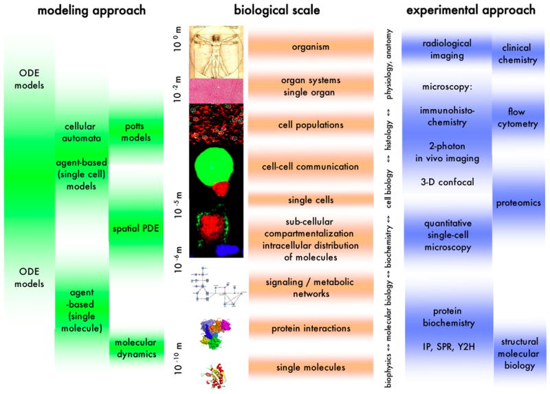
A diagrammatic representation of different biological scales and their associated modeling techniques and experimental approaches. Abbreviations: ODE: ordinary differential equation; PDE: partial differential equation; IP: immuno-precipitation; SPR: surface plasmon resonance; Y2H: yeast two-hybrid.

Many software tools nowadays make it possible to formulate and simulate quantitative models of cellular signaling processes without having to invest effort into the more technical aspects (such as integrating differential equations) of calculating time courses of biochemical concentrations [6, 14–23]. Reflecting the growing appreciation of the fact that molecular interactions are stochastic events, many of these tools contain algorithms that allow the modeler to simulate the temporal evolution of a model not just as a deterministic process but, if necessary, also as a sequence of discrete stochastic molecular events. In addition to approaches that use some implementation of Gillespie’s Monte Carlo algorithm [24, 25] which provides a method to simulate the fluctuations in species abundances there are approaches that explicitly simulate the stochastic dynamics of single molecules [26]. Neglecting the inherently stochastic nature of molecular interactions is justified when the contributions of stochastic fluctuations are too small to have a significant influence on the simulated systems’ behavior. A useful rule of thumb is that the fluctuations around the mean of a molecular binding state, for instance the number of occupied receptors of a given type, are typically of the order of the square root of the number of available molecules of that type. For 100 receptors, the number of occupied receptors would thus stochastically fluctuate 10% up and down. If the signaling network downstream of the receptors is sensitive enough, these fluctuations may have biological consequences. For 10,000 receptors and a high enough concentration of the ligand the receptor signal would fluctuate by only 1%. Depending on the sensitivity of the system, a deterministic simulation – far less time consuming than a stochastic simulation – may then be in order. It should be noted that stochastic effects are not only important on the molecular scale. Depending on the accessibility of their DNA different individual cells of a given phenotype may express varying numbers of copies of their proteins [27]. These random variations translate into variations in the responsiveness of the cells toward external signals.

With increasing complexity of diagrams depicting molecular interaction networks [28] extracting information such as the temporal or causal hierarchy of signaling events becomes increasingly difficult. Molecular interaction maps with well-defined symbols for specific types of molecular species, phosphorylation states and interactions aim at establishing a framework for visualizing the structure of signaling processes [29]. Most modeling tools for intracellular signaling networks assume well-mixed biochemical systems without taking into account spatial aspects such as the non-homogeneous intracellular distribution of signaling components. Mechanisms like membrane recruitment of signaling components and the interplay between membrane proximal activation and cytosolic deactivation, in addition to intracellular compartmentalization can make the assumption of a well-mixed homogeneous cellular biochemistry rather unrealistic [30]. However, due to the greater conceptual and computational effort required for spatially resolved simulations only few generic modeling tools are capable of simulating such spatial aspects thereby linking the scales of signaling networks and sub-cellular distribution of molecular components on the multi-scale map (Fig. 1).

Some tools simulate intracellular reaction-diffusion with the help of partial differential equations [6, 18] that, in addition to time, include space as a variable. For these approaches, the intracellular space is divided into volume elements (this process is frequently called ‘discretization’ of the space). Molecular species in different volume elements are (computationally) treated like different species with the diffusion between volume elements being equivalent to inter-species transitions. With increasing computer power, it is becoming feasible to simulate stochastic changes of particle numbers in the volume elements representing intracellular space through generalizations of Gillespie’s algorithm [24] that include molecular diffusion events (transitions from one volume element to another) in addition to chemical reactions [31]. For not too large regions of intracellular space, cellular membranes or cell-cell contact regions such as neuronal synapses, the stochastic diffusional trajectories of single molecular particles and their interactions may be simulated [32, 33].

Models that focus on cell state transitions and their consequences for inter-cellular communication – as opposed to details of intracellular biochemistry – are frequently formulated in terms of finite state automata. Finite state automata models consist of a set of states and rules specifying how each state reacts to input signals, for instance by switching from one state to another. Adding a spatial aspect to automata models, cellular automata consist of grids of ‘cells’ that switch between states based on the states of their neighbor ‘cells’ [34]. Generalizations of the simple structure of cellular automata treat the single ‘cells’ as agents that can carry their states with them as they move on the grid representing extracellular space. Such agent-based models have been used for computer simulations of multi-cellular systems such as the adaptive immune system [35–37], excitable tissues [38] or populations of migrating cells [39], while others aim to provide generic platforms for studying how tissue-, organ- and organism-level biological phenomena may emerge from the behavior of simple, locally interacting cells [40]. While cellular automata models treat the single ‘cells’ in their simulations as entities with fixed shape and size, Potts model simulations aim at reproducing the shape changes cells undergo due to mechanical contact with neighbor cells or extracellular matrices [41–43]. The boundary between (frequently agent-based) simulations of spatially confined multicellular systems and dynamic models of cell populations characterized mainly by their phenotype is somewhat diffuse. In those situation in which a model does not have to keep track of single-cellular states, cell population simulations are more efficiently performed based on differential equations than based on discrete agents. Differential equation models of cell populations describe how the change per unit time of the size of each population (that is, the number of cells in the population) depends on cell proliferation, death, differentiation and on interactions with other cell types or infectious agents [44–46]. Sometimes, such models include translocation of cells between spatial compartments – which, in the mathematical description, is very similar to state transitions. Dynamic differential equation based models have their roots in general population dynamical modeling. Predator-prey models [47], in particular, have been used to numerically investigate the influences of negative and positive interactions between cell populations [48].

The two paradigmatic fields with a long-standing tradition of multi-scale modeling efforts are heart [49] and brain research [50]. Performing computational studies in these disciplines typically means facing the challenges of multi-scale models because the functions of heart and brain can only be understood by investigating the cooperative actions of large numbers of cells. Fortunately, for the cell types and their modes of communication in heart and brain tissue, useful models can be formulated and valuable insights gained based on strong simplifications and abstractions many of which include separation of biochemical from electrophysiological (and in the case of the heart: mechanical) cellular behavior. Recent modeling advances in neurobiology have produced models comprising millions of neurons and much larger numbers of synapses with different classes of functionality [51] and models of cardiac dynamics are now capable of reproducing and analyzing many aspects of whole heart behavior [49, 52–54]. Among the challenges that the disciplines of computational neurology and cardiology will now face is to develop models that use realistic couplings between intracellular biochemistry and cellular electrophysiology.

4. Developing a multi-scale model of single-cellular signaling and multi-cellular communication with Simmune

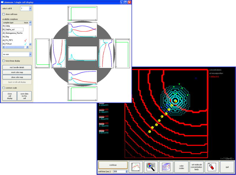
The modeling and simulation software Simmune [6, 13] was developed to connect the scale of interactions between molecular binding sites to the scale of (spatially resolved) intracellular biochemistry to the scale of whole-cell behavior and beyond, to the scale multi-cellular systems by combining reaction network simulations with rules (or mechanisms) for state transitions such as used in automata models. The software performs most of the bridging between the scales automatically. Based on the user inputs defining molecular properties such as diffusion coefficients and whether a molecule type represents a trans-membrane receptor or a membrane anchored adaptor or a freely diffusing cytosolic component and defining interactions between molecular binding sites and the (enzymatic) transformations they mediate the software automatically generates the resulting network of interacting molecular complexes and their kinetic relationships. Defining these properties does not require writing computer scripts or reaction equations. Instead, icononographic representations of molecules and molecular complexes are used (see Fig. 2a). After the building blocks of the extra- and intra-cellular biochemistry have been defined they can be used to specify the phenotype and the behavior of cells by defining the initial molecular contents of cells and, importantly, by defining cellular stimulus-response mechanisms that link sets of conditions (stimuli) to sets of actions (responses) that will be performed by the cells. A simple stimulus response mechanism could, for instance, link a supra-threshold ligation of a specific receptor in a user-defined region of the cytoplasmic membrane to cellular proliferation, death or differentiation. In this way, the scale of (sub-)cellular biochemistry can be coupled to the scale of whole cell behavior using phenomenological shortcuts (see section 2). During a simulated experiment, cells can be positioned into simulated 3D extracellular compartments and can interact through their surface receptors and can be exposed to extracellular molecular stimuli. The intracellular biochemistry of each cell can be investigated in detail and can be linked to the history of its movements and of the stimuli it received through other cells or extracellular molecules (see Fig. 2b).

Figure 2. Screenshots of the user interface of the Simmune modeling and simulation software.

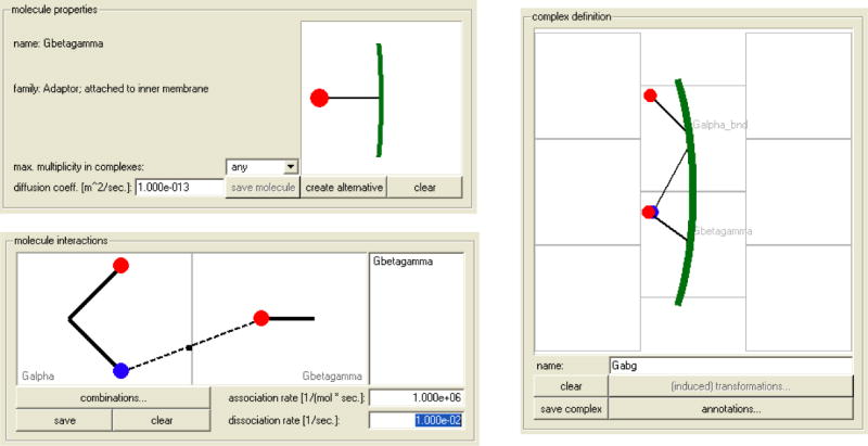
(A) Defining molecular properties, interactions and multi-molecular complexes using iconographic representations for molecules and their binding sites. Binding possibilities between molecular binding sites can be defined by drawing a line between the sites and then specifying the interaction rates (for association and dissociation). Based on these user inputs the software generates the complete network of multi-molecular complexes. The same iconographic symbols as were used to specify molecular properties can be used to define (right hand panel) for which complexes (out of all the complexes of the automatically constructed signaling network) the simulation should report concentration time courses.

(B) Right hand panel: Cells (green and dark-blue disks) are moving in a concentration gradient of a chemoattractant (indicated by red lines). Receptors on the cells’ surfaces bind to the chemoattractant and signal into an intracellular chemosensing signaling network. The biochemical polarization of the responding cells is coupled to a stimulus-response mechanism for directed movement of the cells along the polarization axis. A second stimulus response mechanism translates supra-threshold ligation of the receptor into secretion of a molecular agent into the extracellular milieu (light blue lines). Cells can be selected for detailed inspection of their intracellular biochemistry by mouse click. The left hand panel shows this display of concentration time courses in different regions of one selected cell.

5. Experiments, multi-scale data, modeling and systems biology

Practically speaking, taking a ‘systems’ approach to a biological problem requires the integration of data collected over multiple scales in an effort to more comprehensively describe a biological process. The aim in such research efforts is to establish an infrastructure for data collection, storage and analysis that provides the basis for computational modeling of a biological system [55, 56]. Such models could in essence be limited to a single scale, but the potential of systems biology will only be realized with the development of multi-scale quantitative models capable of predicting the physiological consequences of interventions at the molecular level.

Almost any biological experiment will produce data that can potentially be incorporated into a multi-scale model, but developing an appreciation of where various types of data fit into a multi-scale modeling environment is a valuable exercise. The following descriptions of data types begins at the finest level of detail describing molecular interactions, working towards data which provides limited or no molecular details, but more accurately reflects a physiological function.

Molecular interactions

Detailed studies of molecular interaction between known components of a biological process might involve assessment of binding and reaction kinetics (SPR, ligand-receptor association), structure of both single proteins and complexes, measurement of post-translation modifications, or accurate quantitation of component concentrations. The number of components involved in a defined process may be expanded through literature survey and/or protein-protein interaction screens.

Network structure

Any effort to connect a detailed molecular interaction model to a description of the contribution of such interactions in a cellular network requires an appreciation that the significance of an in vitro determination is context dependent. Assuming that co-expression of the said components in any cell system under study is a given, it is important to establish that the components can interact in the cell (biochemical fractionation, co-immunoprecipitation) and that they have overlapping spatial distribution (fluorescence microscopy). Stimulus dependent regulation of component levels (expression arrays, next-generation sequencing) is also a key determinant of network structure and dynamics, as is the activity state of components (associated inhibitors, activity dependent post-translational modifications).

Network control of cellular function

Expression arrays, proteomic and flow cytometry approaches and quantitative microscopy provide important data sets for prediction of network function in different cellular contexts. Testing of such predictions ultimately rests on perturbations that can establish network sensitivity. Use of small molecules, genetic knockouts, RNA interference and expression of dominant negatives are currently popular approaches that can identify key nodes in a network. Epistasis mapping can also be used to establish whether redundancy in key components confers robustness to the system.

Cellular control of physiological function

Can a model describing network structure and sensitivity nodes established using in vitro or cell-based assays predict higher order cell-cell interactions and physiological phenomena? The immune system is especially well-suited to address such questions [57] as it can be reconstituted with specific cell types harboring specific genetic modifications. Thus it allows us to ask whether computational models derived from molecular data linked through the multiple scales described here can explain or predict cellular function and cell-cell interactions in vivo. The ultimate goal in this regard would be to develop a predictive multi-scale model of how an organism interacts with an infectious agent, and how the genetics of both the pathogen and the host affects the outcome of such an infection.

6. Putting the pieces together: integrating models, simulations and data across scales

Due to the inherent heterogeneity of their components developing successful multi-scale models is, above all, an exercise in integrating various simulation techniques, various experimental techniques and data from heterogeneous sources. Projects like cytoscape (http://www.cytoscape.org) or the geWorkbench of the National Center for the Multiscale Analysis of Genomic and Cellular Networks (MAGNet) (http://magnet.c2b2.columbia.edu/index.php) aim at providing frameworks for such integration efforts.

On the computational side, model sharing standards such as SBML [58] and CellML [59] are evolving to accommodate new modeling capabilities (generation of reaction networks from molecular binding site interactions, spatially resolved computational representations of intracellular biochemistry etc.). While variations in experimental protocols and measurements are unavoidable, in the future, increasing emphasis will have to be put on improving standardization of ontology and data reporting to take us closer to the grand vision for multi-scale modeling and systems biology – to achieve seamless integration of models, simulation techniques and the necessary data to build and test the models.

References

- 1.Burrage K, Hood L, Ragan MA. Advanced computing for systems biology. Brief Bioinform. 2006;7(4):390–8. doi: 10.1093/bib/bbl033. [DOI] [PubMed] [Google Scholar]
- 2.Hunter PJ, Crampin EJ, Nielsen PM. Bioinformatics, multiscale modeling and the IUPS Physiome Project. Brief Bioinform. 2008;9(4):333–43. doi: 10.1093/bib/bbn024. [DOI] [PubMed] [Google Scholar]
- 3.Parent CA, Devreotes PN. A cell’s sense of direction. Science. 1999;284(5415):765–70. doi: 10.1126/science.284.5415.765. [DOI] [PubMed] [Google Scholar]
- 4.Iijima M, Huang YE, Devreotes P. Temporal and spatial regulation of chemotaxis. Dev Cell. 2002;3(4):469–78. doi: 10.1016/s1534-5807(02)00292-7. [DOI] [PubMed] [Google Scholar]
- 5.Merlot S, Firtel RA. Leading the way: Directional sensing through phosphatidylinositol 3-kinase and other signaling pathways. J Cell Sci. 2003;116(Pt 17):3471–8. doi: 10.1242/jcs.00703. [DOI] [PubMed] [Google Scholar]
- 6.Meier-Schellersheim M, et al. Key role of local regulation in chemosensing revealed by a new molecular interaction-based modeling method. PLoS Comput Biol. 2006;2(7):e82. doi: 10.1371/journal.pcbi.0020082. [DOI] [PMC free article] [PubMed] [Google Scholar]
- 7.Xu X, et al. Locally controlled inhibitory mechanisms are involved in eukaryotic GPCR-mediated chemosensing. J Cell Biol. 2007;178(1):141–53. doi: 10.1083/jcb.200611096. [DOI] [PMC free article] [PubMed] [Google Scholar]
- 8.Ma L, et al. Two complementary, local excitation, global inhibition mechanisms acting in parallel can explain the chemoattractant-induced regulation of PI(3,4,5)P3 response in dictyostelium cells. Biophys J. 2004;87(6):3764–74. doi: 10.1529/biophysj.104.045484. [DOI] [PMC free article] [PubMed] [Google Scholar]
- 9.Craver C. When mechanistic models explain. Synthese. 2006;153(3):355–376. [Google Scholar]
- 10.Grossman Z, et al. Concomitant regulation of T-cell activation and homeostasis. Nat Rev Immunol. 2004;4(5):387–95. doi: 10.1038/nri1355. [DOI] [PubMed] [Google Scholar]
- 11.Aloy P, Russell RB. Structural systems biology: modelling protein interactions. Nat Rev Mol Cell Biol. 2006;7(3):188–97. doi: 10.1038/nrm1859. [DOI] [PubMed] [Google Scholar]
- 12.Karplus M, Kuriyan J. Molecular dynamics and protein function. Proc Natl Acad Sci U S A. 2005;102(19):6679–85. doi: 10.1073/pnas.0408930102. [DOI] [PMC free article] [PubMed] [Google Scholar]
- 13.Meier-Schellersheim M, Mack G. SIMMUNE, a tool for simulating and analyzing immune system behavior. 1999 cs.MA/9903017. [Google Scholar]
- 14.Blinov ML, et al. BioNetGen: software for rule-based modeling of signal transduction based on the interactions of molecular domains. Bioinformatics. 2004;20(17):3289–91. doi: 10.1093/bioinformatics/bth378. [DOI] [PubMed] [Google Scholar]
- 15.Lok L, Brent R. Automatic generation of cellular reaction networks with Moleculizer 1.0. Nat Biotechnol. 2005;23(1):131–6. doi: 10.1038/nbt1054. [DOI] [PubMed] [Google Scholar]
- 16.Mendes P. GEPASI: a software package for modelling the dynamics, steady states and control of biochemical and other systems. Comput Appl Biosci. 1993;9(5):563–71. doi: 10.1093/bioinformatics/9.5.563. [DOI] [PubMed] [Google Scholar]
- 17.Tomita M, et al. E-CELL: software environment for whole-cell simulation. Bioinformatics. 1999;15(1):72–84. doi: 10.1093/bioinformatics/15.1.72. [DOI] [PubMed] [Google Scholar]
- 18.Slepchenko BM, et al. Quantitative cell biology with the Virtual Cell. Trends Cell Biol. 2003;13(11):570–6. doi: 10.1016/j.tcb.2003.09.002. [DOI] [PubMed] [Google Scholar]
- 19.Shapiro BE, et al. Cellerator: extending a computer algebra system to include biochemical arrows for signal transduction simulations. Bioinformatics. 2003;19(5):677–8. doi: 10.1093/bioinformatics/btg042. [DOI] [PubMed] [Google Scholar]
- 20.Hoops S, et al. COPASI--a COmplex PAthway SImulator. Bioinformatics. 2006;22(24):3067–74. doi: 10.1093/bioinformatics/btl485. [DOI] [PubMed] [Google Scholar]
- 21.Dhar P, et al. Cellware--a multi-algorithmic software for computational systems biology. Bioinformatics. 2004;20(8):1319–21. doi: 10.1093/bioinformatics/bth067. [DOI] [PubMed] [Google Scholar]
- 22.Hucka M, et al. The ERATO Systems Biology Workbench: enabling interaction and exchange between software tools for computational biology. Pac Symp Biocomput. 2002:450–61. doi: 10.1142/9789812799623_0042. [DOI] [PubMed] [Google Scholar]
- 23.Vayttaden SJ, Bhalla US. Developing complex signaling models using GENESIS/Kinetikit. Sci STKE. 2004;2004(219):14. doi: 10.1126/stke.2192004pl4. [DOI] [PubMed] [Google Scholar]
- 24.Gillespie DT. A general method for numerically simulating the stochastic time evolution of coupled chemical reactions. J Comp Phys. 1976;22:403–434. [Google Scholar]
- 25.Li H, et al. Algorithms and software for stochastic simulation of biochemical reacting systems. Biotechnol Prog. 2008;24(1):56–61. doi: 10.1021/bp070255h. [DOI] [PMC free article] [PubMed] [Google Scholar]
- 26.Le Novere N, Shimizu TS. STOCHSIM: modelling of stochastic biomolecular processes. Bioinformatics. 2001;17(6):575–6. doi: 10.1093/bioinformatics/17.6.575. [DOI] [PubMed] [Google Scholar]
- 27.Sigal A, et al. Variability and memory of protein levels in human cells. Nature. 2006;444(7119):643–6. doi: 10.1038/nature05316. [DOI] [PubMed] [Google Scholar]
- 28.Oda K, Kitano H. A comprehensive map of the toll-like receptor signaling network. Mol Syst Biol. 2006;2:2006 0015. doi: 10.1038/msb4100057. [DOI] [PMC free article] [PubMed] [Google Scholar]
- 29.Kohn KW, et al. Molecular interaction maps of bioregulatory networks: a general rubric for systems biology. Mol Biol Cell. 2006;17(1):1–13. doi: 10.1091/mbc.E05-09-0824. [DOI] [PMC free article] [PubMed] [Google Scholar]
- 30.Kholodenko BN. Cell-signalling dynamics in time and space. Nat Rev Mol Cell Biol. 2006;7(3):165–76. doi: 10.1038/nrm1838. [DOI] [PMC free article] [PubMed] [Google Scholar]
- 31.Hattne J, Fange D, Elf J. Stochastic reaction-diffusion simulation with MesoRD. Bioinformatics. 2005;21(12):2923–4. doi: 10.1093/bioinformatics/bti431. [DOI] [PubMed] [Google Scholar]
- 32.Coggan JS, et al. Evidence for ectopic neurotransmission at a neuronal synapse. Science. 2005;309(5733):446–51. doi: 10.1126/science.1108239. [DOI] [PMC free article] [PubMed] [Google Scholar]
- 33.Lipkow K, Andrews SS, Bray D. Simulated diffusion of phosphorylated CheY through the cytoplasm of Escherichia coli. J Bacteriol. 2005;187(1):45–53. doi: 10.1128/JB.187.1.45-53.2005. [DOI] [PMC free article] [PubMed] [Google Scholar]
- 34.Wolfram S. Theory and Applications of Cellular Automata. Addison-Wesley; 1986. [Google Scholar]
- 35.Celada F, Seiden PE. A computer model of cellular interactions in the immune system. Immunol Today. 1992;13(2):56–62. doi: 10.1016/0167-5699(92)90135-T. [DOI] [PubMed] [Google Scholar]
- 36.Mata J, Cohn M. Cellular automata-based modeling program: synthetic immune system. Immunol Rev. 2007;216:198–212. doi: 10.1111/j.1600-065X.2007.00511.x. [DOI] [PubMed] [Google Scholar]
- 37.Efroni S, Harel D, Cohen IR. Emergent dynamics of thymocyte development and lineage determination. PLoS Comput Biol. 2007;3(1):e13. doi: 10.1371/journal.pcbi.0030013. [DOI] [PMC free article] [PubMed] [Google Scholar]
- 38.Bartocci E, et al. CellExcite: an efficient simulation environment for excitable cells. BMC Bioinformatics. 2008;9 Suppl 2:S3. doi: 10.1186/1471-2105-9-S2-S3. [DOI] [PMC free article] [PubMed] [Google Scholar]
- 39.Hatzikirou H, Deutsch A. Cellular automata as microscopic models of cell migration in heterogeneous environments. Curr Top Dev Biol. 2008;81:401–34. doi: 10.1016/S0070-2153(07)81014-3. [DOI] [PubMed] [Google Scholar]
- 40.Amir-Kroll H, et al. GemCell: A generic platform for modeling multi-cellular biological systems. Theoretical Computer Science. 2008;391:276–290. [Google Scholar]
- 41.Graner F, Glazier JA. Simulation of biological cell sorting using a two-dimensional extended Potts model. Phys Rev Lett. 1992;69(13):2013–2016. doi: 10.1103/PhysRevLett.69.2013. [DOI] [PubMed] [Google Scholar]
- 42.Beltman JB, et al. Lymph node topology dictates T cell migration behavior. J Exp Med. 2007;204(4):771–80. doi: 10.1084/jem.20061278. [DOI] [PMC free article] [PubMed] [Google Scholar]
- 43.Izaguirre JA, et al. CompuCell, a multi-model framework for simulation of morphogenesis. Bioinformatics. 2004;20(7):1129–37. doi: 10.1093/bioinformatics/bth050. [DOI] [PubMed] [Google Scholar]
- 44.Layden TJ, et al. Mathematical modeling of viral kinetics: a tool to understand and optimize therapy. Clin Liver Dis. 2003;7(1):163–78. doi: 10.1016/s1089-3261(02)00063-6. [DOI] [PubMed] [Google Scholar]
- 45.McQueen PG, McKenzie FE. Host control of malaria infections: constraints on immune and erythropoeitic response kinetics. PLoS Comput Biol. 2008;4(8):e1000149. doi: 10.1371/journal.pcbi.1000149. [DOI] [PMC free article] [PubMed] [Google Scholar]
- 46.Althaus CL, De Boer RJ. Dynamics of immune escape during HIV/SIV infection. PLoS Comput Biol. 2008;4(7):e1000103. doi: 10.1371/journal.pcbi.1000103. [DOI] [PMC free article] [PubMed] [Google Scholar]
- 47.Volterra V. Variazioni e uttuazioni del humero d’individui in specie animali conviventi [Variations and uctuations of the number of individuals in animal species living together] Mem Acad Lincei. 1926;2:31–113. [Google Scholar]
- 48.Ludewig B, et al. Determining control parameters for dendritic cell-cytotoxic T lymphocyte interaction. Eur J Immunol. 2004;34(9):2407–18. doi: 10.1002/eji.200425085. [DOI] [PubMed] [Google Scholar]
- 49.Kerckhoffs RCP, et al. Computational methods for cardiac electromechanics. Proc IEEE. 2006;94:769–783. [Google Scholar]
- 50.Le Novere N. The long journey to a Systems Biology of neuronal function. BMC Syst Biol. 2007;1:28. doi: 10.1186/1752-0509-1-28. [DOI] [PMC free article] [PubMed] [Google Scholar]
- 51.Izhikevich EM, Edelman GM. Large-scale model of mammalian thalamocortical systems. Proc Natl Acad Sci U S A. 2008;105(9):3593–8. doi: 10.1073/pnas.0712231105. [DOI] [PMC free article] [PubMed] [Google Scholar]
- 52.Noble D. Computational models of the heart and their use in assessing the actions of drugs. J Pharmacol Sci. 2008;107(2):107–17. doi: 10.1254/jphs.cr0070042. [DOI] [PubMed] [Google Scholar]
- 53.Watanabe H, Sugiura S, Hisada T. The looped heart does not save energy by maintaining the momentum of blood flowing in the ventricle. Am J Physiol Heart Circ Physiol. 2008;294(5):H2191–6. doi: 10.1152/ajpheart.00041.2008. [DOI] [PubMed] [Google Scholar]
- 54.Noble D. From the Hodgkin-Huxley axon to the virtual heart. J Physiol. 2007;580(Pt 1):15–22. doi: 10.1113/jphysiol.2006.119370. [DOI] [PMC free article] [PubMed] [Google Scholar]
- 55.Albeck JG, et al. Collecting and organizing systematic sets of protein data. Nat Rev Mol Cell Biol. 2006;7(11):803–12. doi: 10.1038/nrm2042. [DOI] [PubMed] [Google Scholar]
- 56.Swedlow JR, Lewis SE, Goldberg IG. Modelling data across labs, genomes, space and time. Nat Cell Biol. 2006;8(11):1190–4. doi: 10.1038/ncb1496. [DOI] [PubMed] [Google Scholar]
- 57.Benoist C, Germain RN, Mathis D. A plaidoyer for ‘systems immunology’. Immunol Rev. 2006;210:229–34. doi: 10.1111/j.0105-2896.2006.00374.x. [DOI] [PubMed] [Google Scholar]
- 58.Hucka M, et al. The systems biology markup language (SBML): a medium for representation and exchange of biochemical network models. Bioinformatics. 2003;19(4):524–31. doi: 10.1093/bioinformatics/btg015. [DOI] [PubMed] [Google Scholar]
- 59.Garny A, et al. CellML and associated tools and techniques. Philos Transact A Math Phys Eng Sci. 2008;366(1878):3017–43. doi: 10.1098/rsta.2008.0094. [DOI] [PubMed] [Google Scholar]