Monte Carlo simulation of photon migration in 3D turbid media accelerated by graphics processing units

Abstract

We report a parallel Monte Carlo algorithm accelerated by graphics processing units (GPU) for modeling time-resolved photon migration in arbitrary 3D turbid media. By taking advantage of the massively parallel threads and low-memory latency, this algorithm allows many photons to be simulated simultaneously in a GPU. To further improve the computational efficiency, we explored two parallel random number generators (RNG), including a floating-point-only RNG based on a chaotic lattice. An efficient scheme for boundary reflection was implemented, along with the functions for time-resolved imaging. For a homogeneous semi-infinite medium, good agreement was observed between the simulation output and the analytical solution from the diffusion theory. The code was implemented with CUDA programming language, and benchmarked under various parameters, such as thread number, selection of RNG and memory access pattern. With a low-cost graphics card, this algorithm has demonstrated an acceleration ratio above 300 when using 1792 parallel threads over conventional CPU computation. The acceleration ratio drops to 75 when using atomic operations. These results render the GPU-based Monte Carlo simulation a practical solution for data analysis in a wide range of diffuse optical imaging applications, such as human brain or small-animal imaging.

1. Introduction

Monte Carlo (MC) methods are a set of statistics-based computational algorithms particularly suitable for simulations of complex systems [1]. Distinct from most model-based techniques which produce solutions by solving a set of differential equations, Monte Carlo methods generate solutions by estimating the probability distribution after launching a large number of independent random trials. Because Monte Carlo method does not require the explicit analytical model of the underlying system, it has been found to be a popular choice for exploring the physics of particle systems, financial simulations and computer visualization.

Modeling photon migration in turbid media is one such area were MC has proven to be a valuable tool [2–5], particularly in bio-optical imaging applications such as brain functional imaging and small-animal imaging [6–9]. Due to the generality and capability of handling arbitrary - especially low-scattering - media, the MC method has been used as the gold-standard in these cases, where efficient and accurate methods are required for simulating photon propagation in heterogeneous human tissue. Although the general analytical model, i.e. the radiative transfer equation (RTE), does exist, solving it for arbitrarily complex media is non-trivial [10]. For highly scattering medium, the diffusion equation (DE) has been known to give comparable accuracy to MC solutions; however, it produces erroneous results for cases where voids or low-scattering regions present, for example, the cerebral spinal fluid (CSF) layer in the brain, the void regions in the lung or cysts in the human breast. Although empirical corrections [6] or hybrid techniques [11,12] were proposed to extend the diffusion model for these scenarios, directly using the MC method in the data analysis is also frequently reported for multi-layered or 3D media [2,4,13]. In addition to its accuracy, the simplicity in implementation and the greatly simplified processing pipelines (such as avoiding the mesh generation as in finite-element modeling [14]) further promote the popularity of MC methods in these applications.

Unfortunately, MC-based photon migration is significantly limited by the low computational efficiency. For a typical domain size in the human head, over an hour or more of computational time is required [4] in comparison to a few seconds for solving the DE [14] or minutes for solving the RTE [15]. Despite a number of optimization techniques being proposed [16] to enhance the efficiency of traditional MC photon migration, it remains to be significantly slower than model-based approaches for day-to-day use.

In the last decade, the rapid advances in the development of multi-core processors have revived the hope of making MC a practical solution for bio-optical modeling. Specifically, massively parallel computing based on graphics processing units (GPU) and the development of general-purpose GPU (GPGPU) programming languages have been rapidly progressing for the purposes of scientific computing and have resulted in enormous computational power with market-available graphics hardware. In the US, a graphic card under $200 may contain more than 200 cores, with each core of comparable floating-point operation speed to a Pentium III class processor and up to 1 gigabyte double-data-rate (DDR) video memory. Combined with the deeply optimized processing pipelines, hierarchical thread structures and extremely low memory latency, GPUs constitute an excellent shared memory parallel computing platform. With the increasing versatility and reduced limitations of the graphic shading language, a number of high-level languages for GPGPU applications, including BrookGPU [17], CUDA [18], Brook+ [19] and the recently emerged OpenCL [20], have become freely available and are continuously gaining popularity among computer developers and research communities. Because of the independent nature of the photon propagation, MC simulation of photon migration is readily parallelizable and ideal for this parallel computing platform. Early success of using GPU and CUDA for MC photon migration has recently been reported by Alerstam et al. [21]. An acceleration ratio of 1000 for a homogeneous medium simulation has been found. Lo et al. recently reported a multi-layered media MC simulation accelerated by specialized hardware [22]. In [23], a GPU-based MCML [2] code was published recently for modeling layered media.

In this paper, we go beyond the recent progress in simulations of homogeneous and multi-layered media [21–23] and report a GPU-accelerated MC simulation for 3D complex media incorporated with efficient parallel random-number generators (RNG) and boundary reflection scheme. We first present the implementation details of this parallel MC algorithm. Many of the challenges raised from 3D simulation, such as global memory access, reflection at 3D boundaries, time-resolved simulations and fluence normalization are discussed. These are followed by the Results section, where we compare the solutions from a semi-infinite medium with simulations and diffusion model. Furthermore, we test the algorithm with a realistic brain anatomy from MRI. The computational efficiency of the proposed method was explored with different compilation and simulation parameters. We conclude the paper by highlighting the key findings from the results and our plans for further development and distribution of the software.

2. Methods

2.1 Structure of the simulation

In Fig. 1, we show a block diagram of this parallel MC simulation processing pipeline in conjunction with the GPU memory structure. In this algorithm, we simultaneously launch a given number of simulation threads (depending on hardware) with each thread simulating a sequence of the photon migration process.

Fig. 1.

Block diagram of the parallel Monte Carlo simulation for photon migration. The curved dashed lines indicate read-only global memory access and curved solid line for read/write access..

In each thread, we propagate a series of simulated photons within the medium to produce a fluence distribution [4]. This process can be briefly summarized as:

1. A photon is first launched at the position of the source along an incident direction vector with an initial packet weight [2] of 1.

2. A scattering length, the distance to the next scattering event site, is computed using the scattering coefficient of the current voxel based on an exponential distribution.

3. The photon packet is stepped one voxel length along the scattering trajectory (if the remaining scattering length is less than one voxel, stop at the end of the trajectory).

4. The packet weight is reduced by the absorption coefficient along that step.

5. The packet weight is added to its current voxel's raw probability, i.e. P(r⃗,t), at a fixed time interval and temporally binned based on user specified time gates.

6. Repeat from step 3 until the photon has traveled the total scattering length.

7. Calculate a new scattering direction vector: the azimuth and zenith scattering angles are computed, respectively, by a random number uniformly distributed in [0, 2π) and a random number between [0, π) following the Henyey-Greenstein phase function [2,4].

8. Repeat from step 2 until the photon exits the domain or reaches the maximum time-gate.

9. Repeat from step 1 until the total number of packet steps or simulated photons is reached.

When using a non-dedicated graphics card for both display and computation, the graphics driver may impose a limit for the run-time of a kernel. In this case, we added an option to allow users to simulate a smaller number of photons per call to keep the run-time within the limit, and run for many repetitions. For each repetition, the GPU RNG is re-seeded using a CPU RNG.

Based on the energy conservation relationship in [4], the raw probability accumulated in the volume is then normalized by

$$F(\overrightarrow{r},t)=P(\overrightarrow{r},t)\frac{E_a/E_t}{\text{∑}_i\text{∑}_{j}P({\overrightarrow{r}}_i,t_j){\mu }_a({\overrightarrow{r}}_i)\Delta V\Delta t}$$ (1)

where P(r⃗,t) is the raw probability (unitless) at position r⃗ and time t ; E_a/E_t is the percentage of the total energy being absorbed by the medium (recorded by tracking the packet weight for each photon); ΔV is the voxel volume (mm³) and Δt is the time-gate length (s); μ_a is the medium absorption coefficient (mm⁻¹). The output, F(r⃗,t_i) (mm⁻²s⁻¹), is the fluence distribution under a unitary source for a specified time-gate.

Another important issue in the above simulation pipeline is Step 5 where we simultaneously update P(r⃗,t) from all active threads. Although the accumulation is a commutative process, when a large number of threads read/write the same global memory location concurrently (termed as the race condition), the GPU may have the risk of missing some of the accumulation events. In [23], atomic operations [18] were used for the accumulation in layered media which ensures the integrity of the data. Unfortunately, atomic operations are computationally expensive and are only supported by more recent graphics cards [23]. Nevertheless, the probability for the race condition is expected to be related to $C_T^2{\int }_V{P}_s(\overrightarrow{r},t)P_s(\overrightarrow{r},t)dr$ where $C_T^2=T\times (T-1)/2$ with T being the number of active threads in a multi-processor (MP) [18], P_s(r⃗,t) is the solution for the media with zero absorption; V represents the volume domain of a voxel. From this relationship, we can see that the probability for the race condition is exponentially reduced with the distance from the source voxel as P_s(r⃗,t) decreases exponentially with distance [4]. In Section 3, we quantitatively evaluate the risk of using non-atomic memory write by tracking the accumulation events in benchmark simulations.

2.2 Parallel pseudo-random number generation

An efficient random number generator (RNG) is critical to MC simulations. In this study, we incorporated the well-known Mersenne-Twister (MT) algorithm and a floating-point-only logistic-lattice (LL) algorithm.

The MT RNG has been widely used for its superior quality and enormous period [24]. Fortunately, an efficient parallel version of MT known as SFMT (SIMD-oriented Fast MT) [25–27], was made available by Mills [28] using a shared-memory implementation. In this implementation, all threads in a thread block [18] share 624 32bit integers as the state vector. For each call for a random number, threads within a thread block synchronize and update the state vector in parallel, and produce random integers uniformly distributed between 0 and 2³²-1 for each thread simultaneously. Please note that un-correlation is not guaranteed between thread blocks, despite they are seeded differently. Theoretically, one can choose an SFMT algorithm with longer state vectors [26] to enforce the thread un-correlation of this RNG.

In addition to MT algorithm, we also explored a floating-point based RNG using a chaotic logistic map [29,30]. This RNG allows us to run the simulation with graphics hardware without integer computation capabilities (pre-DirectX 9 hardware), and with higher computational efficiency as a result of extensively optimized 32bit floating-point operations in graphics hardware [18]. More details of this RNG can be found in the Appendix. A logistic lattice with a size of 5 (LL5) is used in our validations in Section 3.

2.3 Boundary reflection

We consider the photon reflection at the exterior boundary of the tissue domain with a simple process. Because we represent the media as a 3D volumetric image, we consider the facets of the boundary voxels as the interfaces for photon reflection. When a photon is moving from tissue domain to the air, the reflection interface will be identified by the method illustrated in Fig. 2: 1) we find the first intersection interface, C₁, along the trajectory by calculating the shortest time-of-flight; 2) if the neighboring voxel of C₁ is an air voxel, we stop, otherwise, we compute the time-of-flight backward from the end point, P_{N + 1}, and find the interface C₂; 3) if the neighboring voxel of C₂ is a medium voxel, we stop, otherwise, based on the interface orientations of C₁ and C₂, the orientation of the last possible interface, C₃, can be uniquely determined as interfaces in x/y/z directions can at most be passed once with a step size of 1 voxel-edge-length, Based on this approach, the reflection interface can be identified as C₂ in Fig. 2(a) and C₃ in Fig. 2(b). The photon propagation direction is then mirrored at the reflection interface. A reflection coefficient is computed based on Fresnel's equation which is multiplied to the packet weight of the photon. To simplify the implementation, we subsequently move the photon position back to the starting point, P_N, inside the tissue domain and let it continue to propagate with the mirrored direction vector.

Fig. 2.

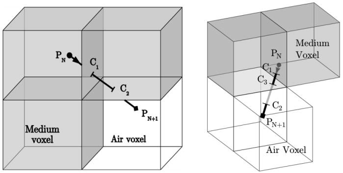
Determination of the reflection interface between the medium (shaded) and air (clear) voxels: (a) case with 2 intersections and (b) case with 3 intersections.

2.4 Time- resolved photon migration

In order to simulate time-domain photon migration problems, we accumulate the photon probability based on the accumulated time-of-flight binned by user specified time-gates, similar to [4]. However, because the simulation is performed entirely on graphics hardware, this requires one to save fluence for all the time-gates in the video (global) memory. In cases where the required memory exceeds the total video memory, we split the target time-gates into groups, and run each group (may contain multiple time-gates) independently. Because the simulations for each time-gate group initiate the photon migration at t=0 at the source position, redundancy may occur when more than one of the groups are simulated.

2.5 GPU memory optimization

In modern graphics hardware, reading and writing global graphics memory can be more than a hundred times slower than reading/writing shared or constant memory (400∼600 clock cycles vs. 4 cycles on nVidia 8800GT [18]). However, the memory holding the medium indices and the fluence data is too big to fit in the shared/constant memory [18]. We attempted to further reduce the memory latency by creating a sub-volume copy of the medium data in the constant memory. By selecting the sub-volume around the source position, this may reduce the global memory reading by 90%. If there are a limited number of tissue types, one can use 1, 2 or 4-bit integers to index the media to further reduce global memory access.

3. Results

We implemented the above parallel MC simulation algorithm in a software package named Monte Carlo eXtreme (MCX) [31] written in CUDA for nVidia™ graphic hardware. We tested the performance of the RNGs and compared the simulation results for a semi-infinite medium with theory. The speed of the proposed algorithm was benchmarked on an nVidia 8800GT (G92). Only integer and single precision computations are used for these implementations. The acceleration rate of the algorithm is tested under various parallel thread numbers and the RNG choice, and compared with a widely-used CPU implementation of a 3D MC algorithm for heterogeneous media, tMCimg, developed by Boas et al. [4]. Because the G92 GPU provides a maximum of 8192 registers per MP and MCX requests 54 registers per thread, the maximum thread number per block is 128 as it has to be multiple of a warp size (32). In all simulations, we report the simulation parameters in the form of (X;Y;Z) where X is the photon moves per thread, Y is the thread number and Z is the repetition count. The total simulated photon number for each case is also mentioned.

3.1 Random number generator performance

Rigorous validation of RNGs is beyond the scope of this work. Here we focus on the basic properties such as speed and serial correlation of the selected RNGs. The speed of the shared-memory MT19937 algorithm has been explored in [26–28]. On the nVidia G92 GPU, the average speed for MT RNG is about 5.7×10⁹ random numbers per second using 128 thread blocks and 128 threads per block.

We tested LL5 RNGs with a single-precision implementation. Using the shuffling scheme in the Appendix, we computed the correlation coefficients between the sequences of a given separation, as shown in Fig. 3. For G92, the speed for LL5 is 137×10⁹ random numbers per second, which is 24 times faster than MT19937.

Fig. 3.

Serial correlation of the logistic-lattice (N=5) based random number generator.

3.2 Comparison to diffusion model and CPU-based simulations

Here we duplicate the simulation setup in [4] to facilitate a straightforward comparison. We simulate a semi-infinite medium using a domain size of 60×60×60 with isotropic 1 mm voxels, filled with medium of absorption coefficient μ_a =0.005 (mm⁻¹), reduced scattering coefficient μ_s′ =1 (mm⁻¹), and anisotropy g=0.01. We used two refractive indices: n=1 and 1.37. For the latter case, the previously described boundary reflection algorithm is used. A point source is located at voxel (30,30,1) pointing toward the +z direction. A total of 10⁸ photons were launched for n=1 (configuration triplet is 6×10⁵;1792;12) and n=1.37 (6×10⁵;1792;160) and the fluence for time window [0,5] ns were computed with a 0.1 ns resolution (i.e. 50 time-gates). Similar to [4], we compare the time-domain and continuous-wave (CW) analytical solutions of the diffusion equation with the simulation outputs. The LL5 RNG was used for these simulations.

We first evaluate the impact of race conditions as discussed in Section 2.1. The ratio between the estimated missing vs. total accumulation events for the region >3 voxels from the source are calculated at various threads and scattering coefficients and are plotted in Fig. 4. The estimated missing events were counted by accumulations using global memory, while the total was counted by using a register for each thread. The domain setup is identical to the following example. From this plot, the maximum missing rate is ∼1% and is expected to produce only minor error in the results. The differences in accuracy and speed for atomic and non-atomic memory access are shown in the remainder of this section. Both methods are provided in MCX.

Fig. 4.

Ratios between the missing and total accumulation events for regions >3 voxels away from the source at various threads and scattering coefficients.

In Fig. 5(a), the time-courses of the fluence at voxel (30,14,9) are shown for n=1 and 1.37. The contour plots on a 2D cross-cut along plane y=30 mm are shown in Fig. 5(b), where the contour lines were calculated by the half-maximum values for time-gates between t=0.1 and 2.1 ns with an increment of 0.5 ns. The CW solution is approximated by integrating the time-domain solutions. The decaying profiles along the radial direction on the interface for n=1 and 1.37 are shown in Fig. 5(c); the 2D contour plots for every 10dB decrease in intensity along plane y=30 mm are shown in Fig. 5(d). We also compare the solutions computed with and without atomic operations near the source in Fig. 5 (e).

Fig. 5.

The comparisons between parallel Monte Carlo algorithm (MCX), tMCimg and the diffusion model for a semi-infinite medium: (a) the time courses at voxel (30,14,9), (b) the contour plots for t=0.1 to 2.1 ns with 0.5 ns step along plane y=30, (c) radial distribution of continuous-wave (CW) solution on the interface, (d) CW fluence contour plot (10 dB spacing) along plane y=30, (e) comparisons between atomic and non-atomic solutions near the source, and (f) domain diagram showing where the results were extracted. In (a), (c) and (e), medium refraction index is 1.37 for simulations with boundary reflections.

3.3 Modeling of an MRI human head atlas

To demonstrate the capability of handling arbitrarily complex media, we run this parallel MC simulation using an MRI scan of human head [32]. The volume dimension of the segmented head anatomy is 181×217×181. A point source is located at voxel (76,68,168) pointing toward the center of the domain. The optical properties for gray matter, white matter, CSF and skin/ scalp/skull were obtained from [33] and [6]. A total number of 1.4×10⁸ photons (10⁶;1792;63) were simulated for the time window [0,3] ns with a step size of 0.2 ns. The cross-cut view of the CW and time-resolved solutions are shown in Fig. 6. The total run-time using a G92 GPU is about 380 seconds with LL5 RNG (including 42 seconds for saving data to disk and 46 seconds GPU- CPU memory transfer).

Fig. 6.

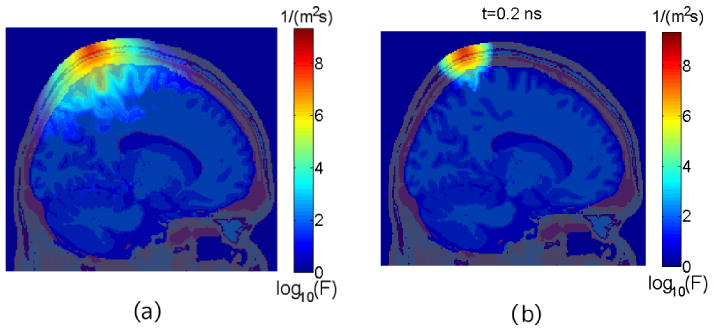
The (a) continuous-wave and (b) time-resolved solutions (Media 1) of photon migration in an MRI head anatomy (transparent overlay). The color map depicts the logarithmic fluence values.

3.4 Speed comparisons and computational scalability

With the mentioned semi-infinite medium and brain atlas simulations, we benchmarked the code with different thread numbers, selection of RNGs and compilation optimization levels, and the corresponding speeds (photons per ms) are summarized in Fig. 7. In the legend, “MT” and “LL5” represent the selection of RNG. A “fast” option was used by linking with CUDA's fast math library (with approximations) in the compilation. We also benchmarked the code with atomic operations enabled. To test the scalability of the simulations, we ran the code using various numbers of threads ranging from 128 to 1792 on a G92 GPU. In this case, the maximum thread number is limited by the maximum threads per MP [18] (constrained by the total register space) and the total MP number. All tests were performed by running 10⁶ photon moves per thread (photon number is ∼1.5×10⁶ at 128 and ∼22×10⁶ at 1792). In comparison, we compiled the CPU implementation, tMCimg, using the “-O3” option with the gcc compiler and double-precision computation on a single core of an Intel 64bit Xeon processor of 1.86GHz. For the semi-infinite medium, the speed for tMCimg is 11.7 photons/ms calculated by dividing 10⁸ photons by the total 8543.7 second run-time; for the brain atlas, the speed is 0.9 photon/ms for 30 hours CPU time. In Fig. 7, we added markers along the z-axis to indicate 100×, 200× and 300× acceleration compared with tMCimg.

Fig. 7.

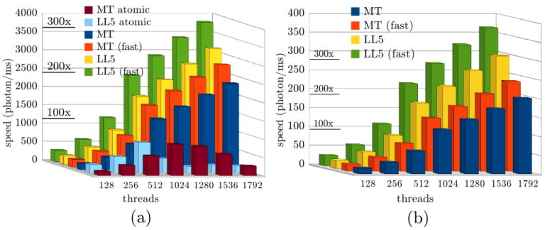
Simulation speed (photon/ms) with various thread numbers and simulation parameters for (a) semi-infinite medium and (b) brain MRI atlas. “MT” - Mersenne-Twister RNG; “LL5” - Logistic-lattice of size 5; “fast” - linked with CUDA's fast math library; “atomic” – with atomic operations (otherwise, without). The acceleration ratio compared with CPU implementation is marked along the z-axis.

We also tested the memory optimization scheme discussed in Section 2.5 for the semi-infinite example. The run-time without this memory optimization is 4.2 seconds for simulating 10⁷ photons (with LL5 and fast math library at 1024 threads). By storing a copy of the sub-volume (10×10×40) around the source with about 4k of constant memory, the simulation surprisingly took about 4.9 seconds to complete. When using 16k constant memory to store a 20×20×40 sub-volume, the run-time extended to 5.5 seconds.

4. Discussion and conclusions

In Fig. 3, the effectiveness of the shuffling strategy is strongly suggested by the reduced correlation coefficients. Because logistic-lattice based RNG involves only floating-point operations, it is an attractive option for graphics hardware that does not support integer computations. Even for those that support integers or CPU-based MC algorithms, this RNG is also an attractive choice for the enhanced speed as suggested in Fig. 7. On average, simulations with LL5 RNG are 33% faster than using the MT algorithm.

In Fig. 5, the results from the parallel MC simulations closely match the outputs from the analytical solutions in both temporal and spatial views, including the case with boundary reflections. There is a slight decrease in the MC solutions at longer time-gates in Fig. 5(a) and larger separations in Fig. 5(c). These differences diminished when running the simulation with a 120×120×120 grid (not shown), indicating that the origin of these differences is the boundary effect [4].

In Fig. 5(e), it appears that only the data points within 2 mm from the source are influenced by the race condition. This once again indicates that the non-atomic method is a valid choice for modeling scattering media away from the source. Despite this, we do include the option to use atomic operations in the MCX software, which can be useful when the source happens to be located inside a low-scattering medium.

From Fig. 4, we do anticipate that the error due to non-atomic-write grows with more threads on newer hardware. In MCX, we implemented an alternative strategy to further reduce the error in these situations. When a photon is within a specified radius from the source, we accumulate the photon weight to a register rather than writing to the global memory. This method can greatly avoid the race conditions near the source, and is expected to give better energy conservation and more accurate solutions elsewhere.

For the boundary reflection scheme, we want to mention that it adds about 20% to 40% more run-time for a fixed number of photon moves, and takes many more photon moves (>10×) to simulate a specified number of photons, as they do not terminate at the boundaries.

The speed benchmark results in Fig. 7 are very encouraging; the dramatic acceleration of the proposed parallel MC algorithm over the single-thread CPU implementation is quite clear. For non-atomic simulations, with a thread number over 1024, the acceleration ratio is between 100 and 250. Using the fast math library in CUDA provides an additional 20% acceleration. This implies that one can obtain a decent MC solution on a typical domain size only within a few minutes on a low-cost graphics card. More importantly, this acceleration ratio is linear-scalable with the number of parallel threads (and MPs), as suggested in Fig. 7. As a result, one may expect to get an additional acceleration factor of 3 or 4 by simply using more recent graphic cards that have more parallel cores or by using multiple GPUs simultaneously. For small animal imaging, this can be even faster due to the smaller domain sizes. For atomic version, the speed does not monotonically increase with more threads. Instead, it peaks around 512 (for LL5) and 1024 (for MT) threads, and then decreases. The peak acceleration in this case is about 75. Although it is about 5 times slower than the peak speed for the non-atomic method, it is still considerably faster than a CPU. Because the atomic method does not scale-up with more threads, we suggest users choosing the non-atomic method whenever possible (possibly with the alternative strategy mentioned above).

Given the dramatic overall improvement in speed, this parallel MC simulation readily becomes a practical option for modeling photon transport in various bio-optical applications. Although it may still be slower than fully optimized diffusion solvers using finite-element or finite-difference methods on CPU [14], considering the fact that it avoids mesh generation and other related pre-/post-processing, MC-based photon migration is overall a competitive alternative for these applications.

It is interesting to mention, from the results in Section 3, our attempt of obtaining further accelerations by packing the medium data into constant (cached) memory failed to achieve the expected speed-up; on the contrary, the efficiency is reduced slightly. By profiling the program, we noticed that the increase in the use of registers for this scheme limits the number of active threads, as indicated by the low GPU occupancy [18]; as a result, the global memory latency becomes less hidden and makes the computation less efficient.

We also want to comment on the apparent discrepancy between the acceleration ratio from Fig. 7 and that of 1000-fold reported by Alerstam et al. [21]. The benchmark reported in [21] is only for homogeneous medium, where no global memory read/write is performed during the simulation of a photon trajectory. Without memory access latency, the 1000-fold acceleration is expected. However, in practice, the medium information cannot fit entirely in the shared or constant memory and global memory latency is unavoidable. In these cases, the acceleration ratio reported in Fig. 7 is more realistic.

A Brook + version of this software is under development for ATI graphics hardware. Both variants of MCX software will soon be available for download at our website [31]. We plan to further improve the efficiency and functionality of the software in the future. We will consider a more accurate boundary representation (B-rep) [34,35], implementing photon reflections at internal tissue boundaries, and further accelerating the computation by optimizing memory and thread utilizations. Additionally, we plan to extend an open-source GPU computing platform BrookGPU to support OpenCL standard. With this support in place, we will migrate the software to this new platform and make it readily usable for most graphics hardware on the market.

Appendix

The logistic map is one of the most intriguing examples to demonstrate chaotic behaviors in a simple system. It can be represented by a recurrence equation as

$$x_{n+1}=f(x_n)=\mu x_n(1-x_n)$$ (2)

where x ∈ [0,1] is a floating-point number and μ is a scalar. It has been shown that for μ = 4, the output sequence from (2) is chaotic: for any given initial value x₀ ∈ [0,1], the output x_n is a random number between [0,1] with probability density function (PDF) of [29]

$$p(x)=\frac{1}{\pi \sqrt{x(1-x)}}$$ (3)

From (3), one can generate a uniform random number in [0,1] by an inverse mapping in form of

$$u_n={cos}^{-1}(1-2x_n)/\pi$$ (4)

In [30], Wagner had shown that this RNG can produce double precision random number sequence with period around 10⁹ depending on the initial values; for single precision, the period is impractically short, typically less than 1000. He also discovered that by using a coupled logistic lattice of size as low as 3, one can produce random number sequences that have sufficient period (>10¹⁰ [30]) even for single precision floating-point numbers. This logistic lattice (LL) method can be described by representing odd numbers (N) of random states by a circular array, and then updating each state using the following equation:

$$x_{n+1}^{imodN}=f(x_n^{imodN})+\nu \left(f(x_n^{i-1modN})-2f(x_n^{imodN})+f(x_n^{i+1modN})\right)$$ (5)

where i mod N is the circular index for the state to be updated; (i − 1) mod N and (i + 1) mod N are the indices of the left and right neighbors, respectively.

We implemented this RNG with N=3 (LL3) and N=5 (LL5) RNG as the alternative choices to the MT RNG. For either case, we update the states using

$$x_{n+1}^{i+pmodN}=f(x_n^{imodN})+\nu \left(f(x_n^{i-1modN})-2f(x_n^{imodN})+f(x_n^{i+1modN})\right)$$ (6)

where the integer shift, p, introduces shuffling to the sequence to reduce the correlation between the subsequence numbers in the output.