A New Image Denoising Framework Based on Bilateral Filter

Abstract

The bilateral filter is a nonlinear filter that does spatial averaging without smoothing edges; it has shown to be an effective image denoising technique in addition to some other applications. There are two main contributions of this paper. First, we provide an empirical study of the optimal parameter selection for the bilateral filter in image denoising applications. Second, we present an extension of the bilateral filter: multi-resolution bilateral filter, where bilateral filtering is applied to low-frequency subbands of a signal decomposed using an orthogonal wavelet transform. Combined with wavelet thresholding, this new image denoising framework turns out to be very effective in eliminating noise in real noisy images. We provide experimental results with both simulated data and real data.

1. INTRODUCTION

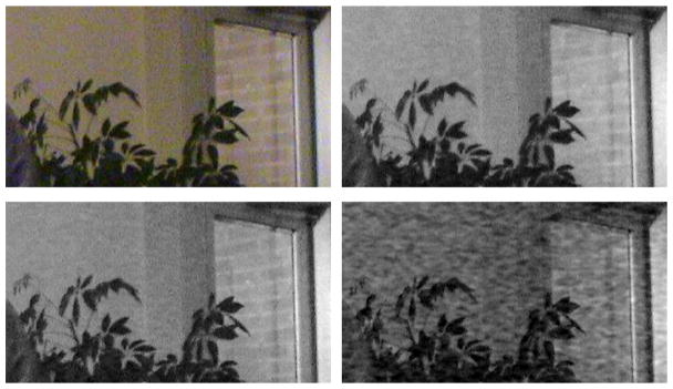
There are different sources of noise in a digital image. For example, dark current noise is due to the thermally generated electrons at sensor sites. It is proportional to the exposure time and highly dependent on the sensor temperature. Shot noise is due the quantum uncertainty in photoelectron generation; and it is characterized by a Poisson distribution. Amplifier noise and quantization noise occur during the conversion of the number of electrons generated to pixel intensities. The overall noise characteristics in an image depends on many factors, including sensor type, pixel dimensions, temperature, exposure time, and ISO speed. Noise is in general channel dependent. Typically, green channel is the least noisy and blue channel is the most noisy channel. In single-chip digital camera, demosaicking algorithms are used to interpolate missing color components; therefore, noise is not independent from pixel to pixel. Noise in a digital image may show low-frequency (coarse-grain) and high frequency (fine-grain) characteristics. (See Figure 1.) High-frequency noise is relatively easier to remove; on the other hand, it is difficult to distinguish between real signal and low-frequency noise.

Figure 1.

Portion of an image captured with a Sony DCR-TRV27; and its red, green, and blue channels. The blue channel is the most degraded channel. The noise apparently has coarse-grain and fine-grain components.

Many denoising methods have been developed over the years, such as the Wiener filter [Wiener 1942], anisotropic diffusion,¹ wavelet thresholding,² bilateral filtering,³ total variation filtering,⁴ and non-local averaging.⁵ Among these methods, wavelet thresholding has become a popular approach. In wavelet thresholding, a signal is decomposed into its approximation (low-frequency) and detail (high-frequency) subbands; as most of the image information is concentrated in few large coefficients, the detail subbands are processed with hard or soft thresholding operations. The critical task in wavelet thresholding is the threshold selection. Various threshold selection strategies have been proposed, for example, VisuShrink,² SureShrink,⁶ and BayesShrink.⁷ In the VisuShrink approach, a universal threshold that is a function of the noise variance and the number of samples is developed based on the minimax error measure. The threshold value in the SureShrink approach is optimal in the Stein’s unbiased risk estimator. The BayesShrink approach determines the threshold value in a Bayesian framework, assuming a Gaussian distribution of the wavelet coefficients. These shrinkage methods have been later improved^8–12 by considering inter-scale and intra-scale correlations of the wavelet coefficients. The method in⁸ models the neighborhoods of coefficients at adjacent positions and scales as Gaussian scale mixture and applies Bayesian least squares technique to update the wavelet coefficients. The method, known as the BLS-GSM method, is one of the best denoising methods in the literature in terms of the mean square error performance.

An alternative to the wavelet-based denosing methods is the bilateral filter.³ The concept of the bilateral filter was earlier presented in¹³ as the SUSAN filter and in¹⁴ as the neighborhood filter. The bilateral filter takes a weighted sum of pixels in a local neighborhood; the weights depend on both the spatial distance and the intensity distance. In this way, edges are preserved well while noise is averaged out. Mathematically, at a pixel location x, the output of a bilateral filter can be formulated as follows:

$$\stackrel{\sim }{I}(\mathbf{x})=\frac{1}{C}\sum _{\mathbf{y}\in \mathcal{N}(\mathbf{x})}{e}^{\frac{-{\left|\right|\mathbf{y}-\mathbf{x}\left|\right|}^2}{2{\sigma }_d^2}}{e}^{\frac{-\mid I(\mathbf{y})-I(\mathbf{x}){\mid }^2}{2{\sigma }_r^2}}I(\mathbf{y}),$$ (1)

where σ_d and σ_r are parameters controlling the fall-off of weights in spatial and intensity domains, (x) is a spatial neighborhood of pixel I(x), and C is the normalization constant:

$$C=\sum _{\mathbf{y}\in \mathcal{N}(\mathbf{x})}{e}^{\frac{-{\left|\right|\mathbf{y}-\mathbf{x}\left|\right|}^2}{2{\sigma }_d^2}}{e}^{\frac{-\mid I(\mathbf{y})-I(\mathbf{x}){\mid }^2}{2{\sigma }_r^2}}.$$ (2)

In addition to image denoising applications, bilateral filters have also been used in texture removal,¹⁵ tone mapping,¹⁶ image enhancement,¹⁷ volumetric denoising,¹⁸ and exposure correction.¹⁹ In,²⁰ it is shown that the bilateral filter is identical to the first iteration of the Jacobi algorithm (diagonal normalized steepest descent) with a specific cost function.²¹ and⁵ relate the bilateral filter with the anisotropic diffusion.¹⁶ describes a fast implementation of the bilateral filter. The technique is based on a piecewise-linear approximation with FFT in the intensity domain and appropriate sub-sampling in the spatial domain.²² later derives an improved acceleration scheme for the filter. They express the bilateral filter in a higher-dimensioned space where the signal intensity is added to the original domain dimensions. The bilateral filter can be expressed as simple linear convolutions in this augmented space followed by two simple nonlinearities, so that they can derive simple criteria for down-sampling the key operations and achieve acceleration.

Although the bilateral filter is being used widely, there is no theoretical study on choosing the optimal values of the parameters σ_d and σ_r. In Section 2, we empirically analyze these parameters as a function of noise variance for image denoising applications. We will show that the value of σ_r is more critical than the value of σ_d; we will in fact show that the optimal value of σ_r (in the mean square sense) is linearly proportional to the standard deviation of the noise. In Section 3, we will propose an extension of the bilateral filter. We will argue that the image denoising performance of the bilateral filter can be improved by incorporating it into a multi-resolution framework. This will be demonstrated in Section 4 with real data.

2. PARAMETER SELECTION FOR THE BILATERAL FILTER

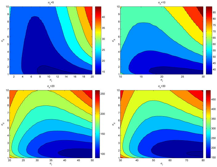
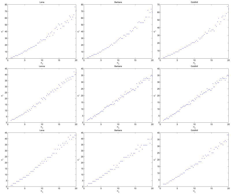
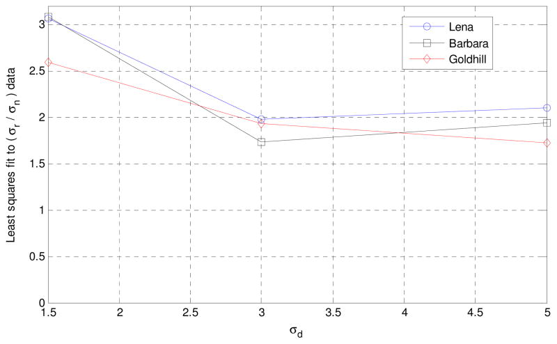
There are two parameters that control the behavior of the bilateral filter. Referring to (1), σ_d and σ_r characterizes the spatial and intensity domain behaviors, respectively. In case of image denoising applications, the question of optimal parameter values has not been answered from a theoretical perspective. In this section, we provide an empirical study of optimal parameter values as a function noise variance. We conducted the following experiment. We added zero-mean white Gaussian noise to some standard images and applied the bilateral filter for different values of the parameters σ_d and σ_r. We repeated this for different noise variances and recorded the mean squared error (MSE). Typical MSE contour plots are given in Figure 2. Examining these plots, we have reached the conclusion that the optimal σ_d value is relatively insensitive to noise compared to the optimal σ_r. While σ_d value can be chosen as constant somewhere around 1.8; σ_r should be chosen as a function of the noise standard deviation σ_n. To see the relationship between σ_n and the optimal σ_r, we set σ_d to some constant values, and plotted the optimal σ_r values as a function of σ_n. Figure 3 shows these plots for three standard images. As seen in these plots, σ_r and σ_n are linearly related to a great degree. The least squares fits to (σ_r/σ_n) data are plotted in Figure 4. It looks for σ_d = 3 or 5, σ_r should be chosen around 2 × σ_n; for σ_d = 1.5; the optimal ratio for (σ_r/σ_n) is around 3.

Figure 2.

The contour plots of the MSE values between the original image and the denoised image for different values σ_d, σ_r, and noise standard deviation σ_n. The test image is the standard gray-scale Lena image of size 512 × 512.

Figure 3.

The optimal σ_r values as function of noise standard deviation σ_n are plotted for three standard images. The image sizes are 512 × 512. The x axis is σ_n while the y axis is the σ_r that produces smallest MSE. From up to the bottom, the three figures in the first row have the σ_d = 1.5, the three figures in the second row have the σ_d = 3, the three figures in the third row have the σ_d = 5.

Figure 4.

Least squares fits to (σ_r/σ_n) data at three σ_d values.

3. A MULTIRESOLUTION IMAGE DENOISING FRAMEWORK BASED ON BILATERAL FILTERING AND WAVELET THRESHOLDING

Multiresolution analysis is an important tool for eliminating noise in signals. It is possible to distinguish between noise (or different frequency components of noise) and image information better at one resolution level than another. This is one of the reasons why wavelet thresholding is so successful in image denoising. Motivated by this fact, we put the bilateral filter in a multiresolution framework. A signal is decomposed into its frequency subbands, and bilateral filtering is applied to the approximation subbands. This method turns out to produce better results than the standard bilateral filter does as effective bilateral window size can be increased without losing details of the image. One can also argue that the coarse-grain noise (as seen in Figure 1) can be eliminated better in a multiresolution framework.

Bilateral filtering works in approximation subbands; however, some noise components can be identified and removed better in detail subbands. Therefore, further improvement can be achieved by including wavelet thresholding into the framework as well. This denoising framework is illustrated in Fig 5. A signal is decomposed into its frequency subbands with wavelet decomposition. The analysis and synthesis filters (L_a, H_a, L_s, and H_s) form a perfect reconstruction filter bank. Two types of filtering are applied on the image. The first one is the bilateral filtering, which is applied to the image and its approximation subbands. The second is the wavelet thresholding, which is applied to the detail subbands of the image.

Figure 5.

Illustration of the proposed method. Image is decomposed into its low- and high-frequency components through analysis filters. Bilateral filter is applied to low-frequency components; wavelet thresholding is applied to high-frequency components. In this illustration, there are two levels of decomposition; the approximation subbands can be decomposed further in an application.

4. EXPERIMENTAL RESULTS

We have conducted some experiments to see the performance of the proposed framework quantitatively and visually. To do quantitative comparisons, we simulated noisy images by adding Gaussian random noise with various standard deviations. These noisy images images were then restored using several algorithms and PSNR results were compared. For visual comparisons, real noisy images were used.

As we discussed earlier, the bilateral filter parameters should be related to the noise variance. There are different ways of estimating the noise levels in images and in different subbands of an image. In our experiments, we used the robust median estimator^{2, 7} to estimate noise variance. The method fits the proposed framework well as it is also wavelet based. For the wavelet thresholding of detail subbands, we used the BayesShrink soft-thresholding technique,⁷ which also uses the same robust median estimator to determine threshold values.

A. PSNR Comparison for Gray-Scale Images

We have done our simulations on standard test images so that the results can be compared with others reported in the literature. We included PSNR results of four methods in Table 1. These methods are the BayesShrink wavelet thresholding,⁷ the original bilateral filter,³ wavelet thresholding⁷ followed by bilateral filter,³ and the proposed method. The results show that proposed method is 0.72dB better than the original bilateral filter and 0.85dB better than the BayesShrink method on average.

Table 1.

PSNR comparison of the BayesShrink method,⁷ the bilateral filter,³ and the proposed method. For the BayesShrink method, the number of decomposition levels is 5. For the bilateral filter, σ_d = 1.8, σ_r = 2 × σ_n, and the window size is 11 × 11. For the proposed method, db8 filters in Matlab are used for 1-level decomposition. σ_d = 1.8 and the window size is 11 × 11. σ_r = σ_n at each level. For the bilateral filter and the proposed method, the noise level is estimated using the robust median estimator.⁷

Input Image	σn	BayesShrink7	Bilateral Filter3	Proposed Method
Barbara 512 × 512	10	31.25	31.28	31.64
	20	27.32	27.09	27.67
	30	25.34	24.96	25.57
Boat 512 × 512	10	31.98	32.13	32.51
	20	28.55	28.49	29.37
	30	26.71	26.27	27.53
Goldhill 512 × 512	10	31.94	32.08	32.46
	20	28.69	28.90	29.57
	30	27.13	27.50	27.93
Peppers 256 × 256	10	31.49	32.25	33.41
	20	27.85	28.87	29.90
	30	25.73	26.70	27.61

B. Visual Comparison for Real Noisy Images

It is well known that the PSNR is not a good representative of visual quality. In case of color images, Euclidean distance in the perceptually uniform CIE-L*a*b* color space gives a better sense of visual quality than the PSNR. It is also a better idea to perform restoration in the CIE-L*a*b* space instead of the RGB space. In our experiments, we applied the proposed method in the CIE-L*a*b* space for color images. Because human visual system is more sensitive to color noise compared to luminance noise, we applied stronger noise filtering (through decomposing into more resolution levels) to color channels a and b than to the luminance channel L.

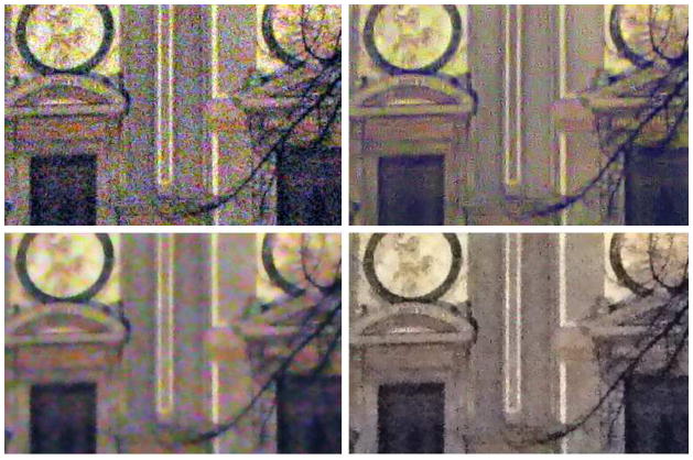
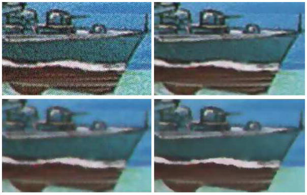
Figures 6 and 7 provide two examples with real data. The results of the BLS-GSM method,⁸ the bilateral filter,³ and the proposed method are given. The BLS-GSM method is considered as one of best denoising algorithms in terms of the PSNR results. However, the proposed method is apparently producing more visually pleasing results than the BLS-GSM method in case of real data.

Figure 6.

(a) Input image obtained from²³ (b) The BLS-GSM result obtained from²³ (c) The bilateral filter³ result (d) Result of the proposed method. For the bilateral filter, σ_d = 1.8, σ_r = 10 × σ_n, and the window size is 11 × 11. For the proposed method, σ_d = 1.8, σ_r = 3 × σ_n at each level, the window size is 11 × 11, and the number of decomposition levels is (1, 4, 4) for the (L, a, b) channels, respectively. The wavelet filters are db8 in MATLAB. The noise parameter σ_n is estimated using the robust median estimator.

Figure 7.

(a) Input image obtained from²³ (b) The BLS-GSM result obtained from²³ (c) The bilateral filter³ result (d) Result of the proposed method. For the bilateral filter, σ_d = 1.8, σ_r = 10 × σ_n, and the window size is 11 × 11. For the proposed method, σ_d = 1.8, σ_r = 3 × σ_n at each level, the window size is 11 × 11, and the number of decomposition levels is (1, 4, 4) for the (L, a, b) channels, respectively. The wavelet filters are db8 in MATLAB. The noise parameter σ_n is estimated using the robust median estimator.

5. CONCLUSIONS

In this paper we present a multiresolution denoising method, which integrates bilateral filtering and wavelet thresholding. We decompose an image into low- and high-frequency components, and apply bilateral filtering on the approximation subbands and wavelet thresholding on the detail subbands. We have found that the optimal σ_r value of the bilateral filter is linearly related to the standard deviation of the noise. The optimal value of the σ_d is relatively independent of the noise power. Based on these results, we estimate the noise variance at each level of the subband decomposition and use the optimal σ_r value for bilateral filtering. We used a specific wavelet thresholding technique; it is possible to improve the results further by using better detail-subband-denoising techniques. The experiments with real data demonstrate the effectiveness of the proposed method in real life.

References

- 1.Perona P, Malik J. Scale-space and edge detection using anistropic diffusion. IEEE Trans Pattern Analysis and Machine Intelligence. 1990 July;12:629–639. [Google Scholar]
- 2.Donoho DL, Johnstone IM. Ideal spatial adaptation by wavelet shrinkage. Biometrika. 1994;81(3):425–455. [Google Scholar]
- 3.Tomasi C, Manduchi R. Bilateral filtering for gray and color images. Proc Int Conf Computer Vision. 1998:839–846. [Google Scholar]
- 4.Rudin LI, Osher S, Fatemi E. Nonlinear total variation based noise removal algorithms. Physica D. 1992;60(1–4):259–268. [Google Scholar]
- 5.Buades A, Coll B, Morel J. Technical Report 2005-04. CMLA; 2005. Neighborhood filters and pde’s. http://www.cmla.ens-cachan.fr/documentation/prepublications/2005.html. [Google Scholar]
- 6.Donoho DL, Johnstone IM, Kerkyacharian G, Picard D. Wavelet shrinkage: Asymptopia? Journal of Royal Statistics Society, Series B. 1995;57(2):301–369. [Google Scholar]
- 7.Chang SG, Yu B, Vetterli M. Adaptive wavelet thresholding for image denoising and compression. Trans Image Processing. 2000 September;9:1532–1546. doi: 10.1109/83.862633. [DOI] [PubMed] [Google Scholar]
- 8.Portilla J, Strela V, Wainwright MJ, Simoncelli EP. Image denoising using scale mixtures of gaussians in the wavelet domain. IEEE Trans Image Processing. 2003 November;12:1338–1351. doi: 10.1109/TIP.2003.818640. [DOI] [PubMed] [Google Scholar]
- 9.Pizurica A, Philips W. Estimating the probability of the presence of a signal of interest in multiresolution single- and multiband image denoising. IEEE Trans Image Processing. 2006 March;15:654–665. doi: 10.1109/tip.2005.863698. [DOI] [PubMed] [Google Scholar]
- 10.Sendur L, Selesnick IW. Bivariate shrinkage functions for wavelet-based denoising exploiting inter-scale dependency. IEEE Trans Signal Processing. 2002 November;50:2744–2756. [Google Scholar]
- 11.Sendur L, Selesnick IW. Bivariate shrinkage with local variance estimation. IEEE Signal Processing Letters. 2002 December;9:438–441. [Google Scholar]
- 12.Luisier F, Blu T, Unser M. A new sure approach to image denoising: Inter-scale orthonormal wavelet thresholding. IEEE Trans Image Processing. 2007 March;16:593–606. doi: 10.1109/tip.2007.891064. [DOI] [PubMed] [Google Scholar]
- 13.Smith SM, Brady JM. Susan - a new approach to low level image processing. Int Journal of Computer Vision. 1997;23:45–78. [Google Scholar]
- 14.Yaroslavsky L. Digital Picture Processing - An Introduction. Springer Verlag; 1985. [Google Scholar]
- 15.Oh BM, Chen M, Dorsey J, Durand F. Image-based modeling and photo editing. Proc. SIGGRAPH; 2001. pp. 433–442. [Google Scholar]
- 16.Durand F, Dorsey J. Fast bilateral filtering for the display of high-dynamic-range images. Proc. SIGGRAPH; 2002. pp. 257–266. [Google Scholar]
- 17.Eisemann E, Durand F. Flash photography enhancement via intrinsic relighting. Proc. SIG-GRAPH; 2004. pp. 673–678. [Google Scholar]
- 18.Wong WCK, Chung ACS, Yu SCH. Trilateral filtering for biomedical images. Proc. International Symposium on Biomedical Imaging, IEEE; 2004. pp. 820–823. [Google Scholar]
- 19.Bennett EP, McMillan L. Video enhancement using per-pixel virtual exposures. ACM Trans on Graphics. 2005;24(3):845–852. [Google Scholar]
- 20.Elad M. On the origin of the bilateral filter and ways to improve it. IEEE Trans Image Processing. 2002 October;11:1141–1151. doi: 10.1109/TIP.2002.801126. [DOI] [PubMed] [Google Scholar]
- 21.Barash D. A fundamental relationship between bilateral filtering, adaptive smoothing, and the nonlinear diffusion equation. IEEE Trans Pattern Analysis and Machine Intelligence. 2002 June;24:844–847. [Google Scholar]
- 22.Paris S, Durand F. A fast approximation of the bilateral filter using a signal processing approach. Proc European Conference on Computer Vision. 2006:568–580. [Google Scholar]
- 23.http://decsai.ugr.es/javier/denoise/, [Dec. 10, 2007].