Localized Components Analysis

Abstract

We introduce Localized Components Analysis (LoCA) for describing surface shape variation in an ensemble of biomedical objects using a linear subspace of spatially localized shape components. In contrast to earlier methods, LoCA optimizes explicitly for localized components and allows a flexible trade-off between localized and concise representations. Experiments comparing LoCA to a variety of competing shape representation methods on 2D and 3D shape ensembles establish the superior ability of LoCA to modulate the locality-conciseness trade-off and generate shape components corresponding to intuitive modes of shape variation. Our formulation of locality in terms of compatibility between pairs of surface points is shown to be flexible enough to enable spatially-localized shape descriptions with attractive higher-order properties such as spatial symmetry.

1 Introduction

The parameterization of an ensemble of biomedical shapes is a key step in a broad array of scientific and medical applications that require quantification of the shape properties of physical objects. In this paper, shape parameterization refers to the problem of converting a representation of the delineating boundary of an object in 2D or 3D into a concise vector of numbers that captures its salient shape characteristics. Converting the potentially complex boundary of a biological object such as an organ or bone into a small set of shape parameters facilitates a variety of statistical analyses, including the characterization of shape variability across an ensemble; comparison of object shape between groups; and the tracking of shape change over time. It is important to present the results of these analyses in an intuitive way to encourage the connection of the shape analysis to domain-specific physical or biological processes. For instance, the interpretability of statistical tests of brain region shape differences between healthy and diseased subjects would be enhanced if differences could be presented in terms of a small number of parameters, each of which represents an easily-grasped aspect of region shape. This could promote interpretations of the shape difference in terms of disease causes or effects.

Our goal is to encourage interpretability of results by generating shape parameterizations that are both concise– capturing salient shape characteristics in a small number of parameters– and spatially localized– accounting for the shape of a spatially restricted sub-region in each parameter. The hypothesis underlying this paper is that spatially-localized and concise shape parameterizations are more intuitive for end users because they allow them to conceptualize object shape in terms a small number of object parts, which are often affected differentially by physical phenomena. In the above example, shape change due to disease processes is known to occur in spatially-localized brain sub-regions in a variety of disorders [1]. In addition, concise parameterizations are attractive because the statistical power of tests on those parameters is reduced as little as possible by corrections for multiple comparisons [2].

We follow the linear subspace paradigm of expressing each shape as a linear combination of prototypical, or basis shapes. That is, if each shape is represented as a vector v_j of the 2m or 3m coordinates of m points sampled from its boundary (i.e., v_j = [v_j,1, v_j,2, ··· v_j,m], v_j,k = [x_k, y_k] for 2D shapes), v_j is approximated as a linear combination of k basis vectors {e₁, e₂, ··· e_k}:

$${\mathbf{v}}_j^k=\sum _{i=1}^k{\alpha }_{j,i}\ast {\mathbf{e}}_i$$

The shape parameters are the coefficients α_j,i. Linear subspace methods are attractive because their linearity in e_i allows them to be manipulated using standard tools from linear algebra.

However, linear subspace methods do not inherently encourage locality. Figure 1 (left) depicts a typical e_i generated by the classical linear subspace method, principal components analysis (PCA), applied to tracings of the corpus callosum (CC), a human brain region. The basis shape summarizes a complex pattern of shape characteristics across the entirety of the CC. Therefore, if the corresponding α_i differs between groups, the explanation of the group difference in physical terms is complex. Figure 1 (right), by contrast, shows a typical e_i generated by the method presented below; differences in the corresponding α_i between groups gives rise to a simple physical explanation in terms of the genu, the CC subregion whose shape is captured by the e_i.

Fig. 1.

Shape characteristics of corpora callosa captured by basis vectors generated with PCA and LoCA. Arrows start at points tracing the average corpus callosum; their magnitudes indicate the degree that points move when the corresponding shape parameter is varied. The PCA vector represents a complex, global pattern of shape characteristics while the LoCA vector focuses on the genu.

We present Localized Components Analysis (LoCA), a method that optimizes the e_i for spatial locality and conciseness simultaneously. It improves on previous linear subspace methods by explicitly optimizing for localized shape parameters and by allowing the user to modulate the tradeoff between locality and conciseness with greater flexibility than previous methods. The resulting shape components could provide succinct summaries of spatially-localized changes to biomedical structures due to a variety of physical phenomena; for example, LoCA could provide a concise summary of the spatially-localized CC shape changes that are thought to accompany diseases such as HIV/AIDS [3]. In primate evolution, LoCA could summarize the shape similarities between the skulls of genetically related species using a few intuitive parameters.

We summarize related techniques in Section 2, and present LoCA in Section 3. A thorough set of experiments in Section 4 shows the intuitiveness and flexibility gained by LoCA over established linear subspace methods when applied to human CC, colobine monkey skulls, and primate humeri (upper arm) bones.

2 Related Work

PCA has been used to find concise bases for shape spaces in medical image analysis [4], morphometrics [5], computer graphics [6], and many other contexts. In PCA, e_i is the ith eigenvector of the covariance matrix of the example v_j vectors; therefore, the e_i are orthogonal and ${\mathbf{v}}_j^k$ is the best k-th order approximation of v_j under the L₂ norm. Two algorithms independently named Sparse PCA (S-PCA) encourage as many entries in e_i to be zero as possible, either by iteratively adjusting the PCA basis [7] or by iteratively constructing sparse orthogonal vectors [8] [9] ⁷. Empirically the e_i often represent shape in a small number of spatially-localized subregions [9] [11]. Similarly, while independent components analysis (ICA) and principal factor analysis (PFA) do not directly optimize a locality-related objective function when estimating e_i, they appear to generate spatially-localized components anyway [12] [13]. Alternatively, pre-defined spatially located regions of interest can be integrated into PCA [14]. Our approach is inspired by S-PCA and follows a similar strategy of adjusting the e_i provided by PCA; but we explicitly optimize for spatially-localized, rather than sparse, e_i. Unlike [14] we allow the decomposition into local regions to emerge from the data.

Networks of localized medial geometric primitives have the potential to capture local shape in a concise set of parameters [15]. We feel that medial and surface-based representations could capture complementary shape information. We note, however, that networks of medial primitives can be challenging to construct in an automated way and may therefore be more labor-intensive than the approach we present.

An alternative approach for determining spatially-localized differences between shape ensembles is to perform statistical tests that compare corresponding v_j,k between groups; spatial maps then color-code each v_j,k by the effect size or p value of the test. Visual inspection of the renderings has revealed spatially-localized shape differences in a variety of medical conditions (see, e.g., [1]); however, m is generally so large that the significance threshold of the statistical tests must be reduced dramatically to guard against detection of spurious group differences [2]. This reduces the sensitivity of spatial mapping techniques to detect subtle shape differences. LoCA uses a linear subspace to reduce the number of variables required for localized shape comparisons, and therefore boost the power of statistical tests.

3 Methods

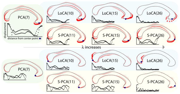
PCA produces the most concise basis possible under the L₂ norm; that is, for each k, ${\sum }_{j=1}^n{\left|\right|{\mathbf{v}}_j-{\mathbf{v}}_j^k\left|\right|}_{L_2}$ is minimized when e₁ ··· e_k are the first k eigenvectors of the covariance matrix of the v_j. We use a formulation of PCA as the minimization of an energy function E_var, and modify it by minimizing E_var + λE_loc, where E_loc is a new energy term that summarizes the spatial locality of the e_i. The λ balances the tradeoff between the competing interests of conciseness and locality (Figure 2).

Fig. 2.

Effect of λ on the first (top) and third (bottom) basis vectors, where vectors are ordered by the amount of shape variation captured. As λ increases, the number of vectors required to capture 90% of the variation (in parentheses) increases. For small values of λ, vectors capturing substantial variation represent a global deformation of the entire shape. As λ is increased, more of the LoCA vectors become local deformations, until the entire basis consists of local vectors. S-PCA becomes sparse more slowly, so that the first vector is still a global deformation on the right. The third vector is sparse, but there is some perturbation across the entire shape. Each vector is accompanied by a graph showing its locality, where every point in the graph represents a point on the outline. The center point is defined as the point minimizing E_loc, as described in Section 3.

Energy Function

Each successive PCA component accounts for as much of the shape variation as possible; that is, the distribution of shape variation over the PCA basis vectors is as concentrated as possible on the leading e_i. More formally, one can define the relative variance β_i of each basis vector e_i as

$${\beta }_i=\frac{{\sum }_{j=1}^n{\langle ({\mathbf{v}}_j-\mu ),e_i\rangle }^2}{{\sum }_{j=1}^n{\left|\right|{\mathbf{v}}_j-\mu \left|\right|}^2}$$

where μ represents the mean of the data vectors v_j. The entropy of the distribution $-{\sum }_{i=1}^k{\beta }_{i}log{\beta }_i$ is minimized, over all orthogonal bases, by the PCA basis, so we define this to be E_var, as in [7]. The S-PCA construction in that paper balances E_var against another energy function that rewards sparse e_i– that is, as many entries as possible in each e_i are encouraged to have zero magnitude. We instead optimize for locality, defining E_loc as follows.

We encourage each e_i to have simultaneous nonzero entries corresponding to points p_i and p_j if and only if p_i and p_j are close to each other. To do so, we introduce a pairwise compatibility matrix B whose entries B[i, j] tend toward 1 when p_i and p_j are near each other, and tend towards 0 when they are distant; we define B below. The B matrix defines a cost function C:

$$C({\mathbf{e}}_i,p_c)=\sum _{j=1}^m{(\mathbf{B}[c,j]-{\left|\right|{\mathbf{e}}_{i,j}\left|\right|}_{L_2})}^{\kappa }$$

The e_i have unit length, so both B[c, j] and ||e_i,j|| vary between 0 and 1. Intuitively, points p_c and p_j contribute significantly to C if: 1. p_c and p_j are incompatible, but e_i,j has high magnitude; or 2. p_c and p_j are compatible, but ||e_i,j|| is close to 0. The exponent κ can take on any value between 1 and 2 to deal with outlier effects. For our experiments, κ was 1.5.

For each basis vector e_i, each p_c yields a different C. We define the locality of e_i using the best possible p_c, that is, the one that minimizes this cost function C. Each p_c differs in the distribution of its distances to all other p_j– for example, points at one end of a humerus bone in Figure 5 are extremely distant from many points at the opposite end of the bone, while points in the middle are not. So we normalize C as follows:

$$E_{\mathit{loc}}=\sum _i\underset{p_c}{min}\frac{C({\mathbf{e}}_i,p_c)}{{max}_{{\mathbf{e}}_{\mathit{bad}}}C({\mathbf{e}}_{\mathit{bad}},p_c)}$$

Fig. 5.

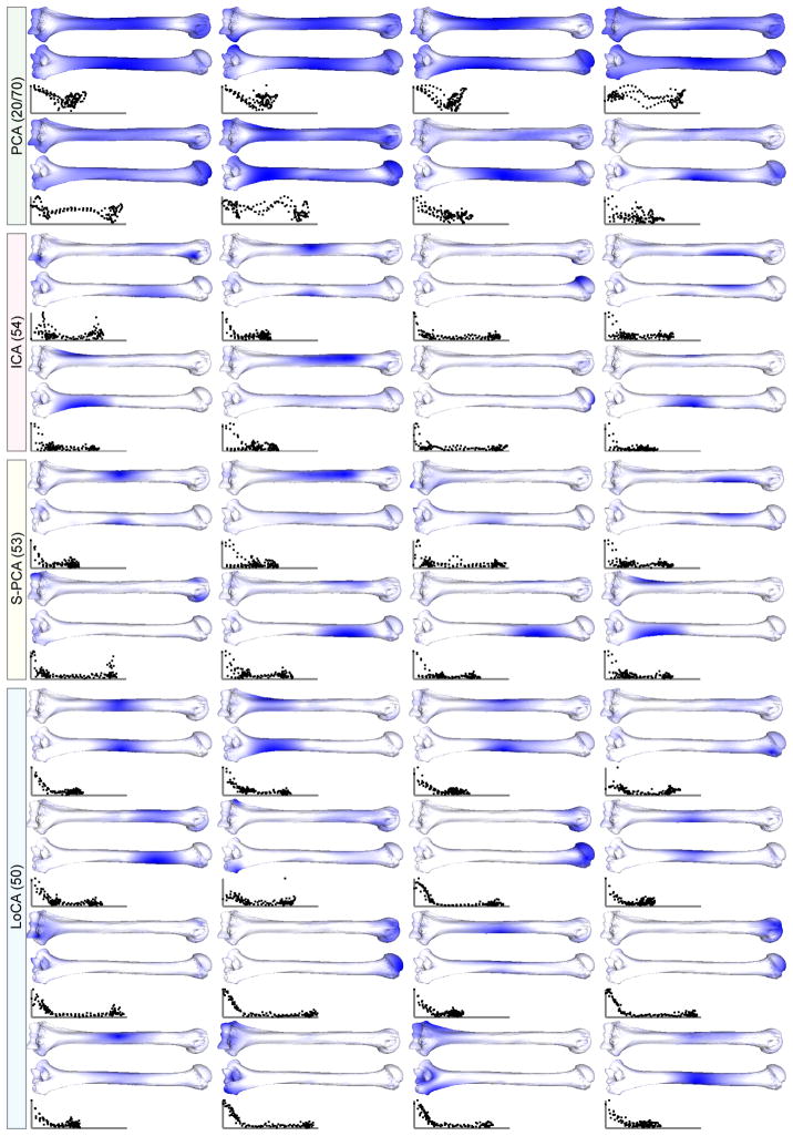
Front and back views of displacements on primate humeri. Displacements of the landmark points are computed using different methods, and then interpolated onto the mesh using a thin-plate-spline. Darker locations indicate greater displacement magnitudes. LoCA components describe the articular surfaces at the two extremities as well as deformations of the shaft.

The denominator for a given p_c is simply Σ_j max(|B[c, j] − 1|, |B[c, j] − 0|)^κ. It needs to be computed only once.

The compatibility B[i, j] can be computed in whatever way is appropriate for the data set; here, B[i, j] is based on the distance D(p_i, p_j) between p_i and p_j. For the CC data set considered below, D is the geodesic distance computed from dense surface meshes. For the 3D humeri and skull data sets, D is computed from an adjacency graph constructed between the landmarks. The compatibility is B[i, j] = f(D(p_i, p_j)), where f is a function that modulates D to adjust its range to [0, 1]. We chose a sinusoidal f that is non-zero over a half-period: $f(x)=0.5(cos(\pi \frac{x}{\rho })+1)$. Larger ρ select for groups of points which co-vary over larger spatial extents. It was set to 0.25 in all of the experiments below.

Optimization

Our optimization procedure is similar to that used in [7]. PCA provides an initial orthonormal basis e, and every possible pair e_i, e_j are rotated together in the two-dimensional plane they span. Because the rotating pair is kept orthogonal to each other and stay in their 2D plane, the basis remains orthonormal throughout optimization. Each pair is rotated by the angle θ that minimizes E_var + λE_loc. The optimal θ is found numerically using Brent’s method [16]. Notice that since E_var and E_loc are both summations of terms that each depend solely on an individual e_i, only the terms corresponding to the current e_i, e_j pair need to be updated during optimization.

The pairs are rotated in decreasing order of shape variation accounted for. The set of all e_i, e_j pairs are adjusted repeatedly, and optimization ceases when adjusting them changes the objective function less than a fixed threshold. Between 50 and 150 iterations were required for each experiment below.

Data preparation

We assume that we are given an ensemble of n objects, each represented by m points on its boundary, and the compatibility matrix B. Overall differences in object scale, rotation and translation over the ensemble are removed through generalized Procrustes alignment [5]. The resulting scaled and aligned data sets are used as input to the above optimization.

4 Results

Below, we compare LoCA to PCA, ICA, and S-PCA on three data sets: CCs, colobine monkey skulls, and humeri from various primates⁸. For each basis, locality is evaluated visually using renderings of the entries in each basis vector, and through locality graphs (see Figure 2). Conciseness of each basis is assessed quantitatively by charting ${\sum }_{j=1}^n{\left|\right|{\mathbf{v}}_j-{\mathbf{v}}_j^k\left|\right|}_{L_2}$ over all k, and more specifically by recording the number of e_i required to capture 90% of shape variation, i.e. reduce this reconstruction error to 10%.

LoCA behavior depends strongly on λ, the parameter that modulates the tradeoff between conciseness and locality. For λ = 0, LoCA reduces to PCA. For small λ, LoCA basis vectors accounting for the highest amounts of shape variation resemble PCA basis vectors, while the rest of the basis is clearly localized (Figure 2). For larger λ, all LoCA basis vectors are local, and the bases require more basis vectors to account for shape variation in the data. In Figures 3, 5, and 6, LoCA and S-PCA basis vectors are depicted for the smallest value of λ for which the bases lacked global basis vectors. S-PCA performs similarly to LoCA for small values of λ, in agreement with earlier S-PCA results [7]. However, S-PCA required a much larger basis– more basis vectors for 10% reconstruction error– before the global basis vectors disappeared; this is likely due to the very high spatial locality of S-PCA basis vectors. Also, more of them were required to describe the deformation of any extended surface region.

Fig. 3.

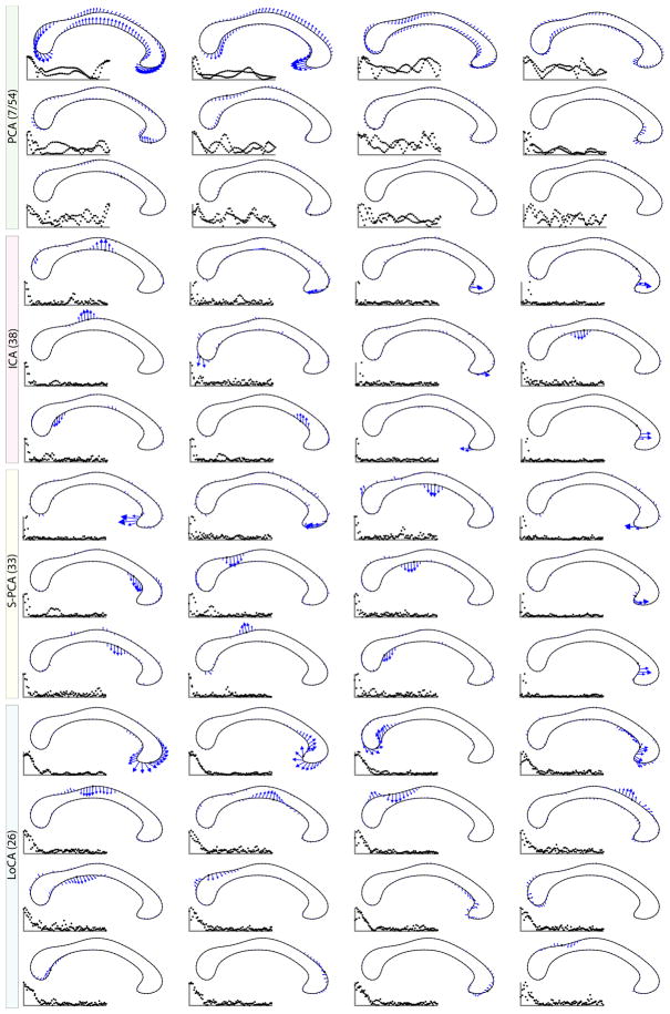
Corpora callosa basis comparison. Out of 54 basis vectors, the first few are shown. LoCA successfully captures the major shape deformations of the genu and splenium in the first four vectors, while both ICA and S-PCA spread this variation over several vectors.

Fig. 6.

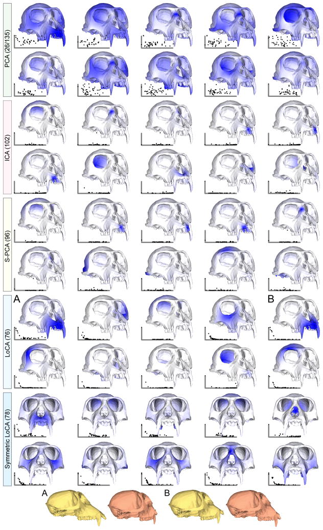
Cranial basis comparison, colored by displacement magnitude. Both S-PCA and ICA produce vectors that move single teeth, while LoCA has vectors that move the entire jaw at once. The side views of vectors A and B differentiate their effects: A represents prognathism (snout elongation), while B represents facial kyphosis (teeth straightening). Note that since the crania are shown from a single angle, vectors representing motion on the bottom of the cranium appear completely white.

Corpora callosa

55 healthy subjects and HIV/AIDS patients received high-resolution magnetic resonance brain scans as part of a previously-described study [3]. The CC was manually traced on all scans using a reliable, repeatable protocol, and sparse landmarks were placed on all traces using the Witelson criteria [17]. 103 point correspondences were established between all CC traces based on the Witelson landmarks using a sparse-to-dense correspondence algorithm [18].

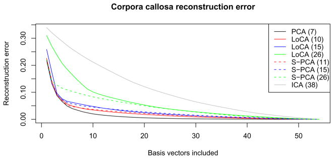
Figure 3 compares the basis vectors from each method that captured the most shape variation. PCA required 7 basis vectors for 90% of shape variation, while ICA required the most at 38. Note the global effects of PCA vectors, the extreme locality of ICA and S-PCA, and the spatially broader effects of LoCA. Major deformations of meaningful CC sub-regions, the genu and splenium, are represented by the first four LoCA vectors, while the next six represent deformations of the corpus callosum’s long central body.

Reconstruction error for all methods is graphed in Figure 4. ICA requires a large number of components for accurate shape reconstruction, and PCA requires the fewest; S-PCA and LoCA require more basis vectors for bases that are more local or sparse (i.e., higher λ). Note, however, that for comparable reconstruction error curves, S-PCA bases tend to contain global shape components while LoCA does not; for example, compare LoCA(26) and S-PCA(26) in Figures 4 and 2.

Fig. 4.

Reconstruction error when using only the first k vectors of the basis. The numbers in parentheses denote the number of vectors required to capture 90% of variation in the data set. LoCA bases are compared with S-PCA bases which have essentially the same reconstruction error for 10, 15, or 26 vectors respectively. These choices correspond to the different λ settings used in Figure 2. Using fewer vectors, S-PCA has lower reconstruction error because the first few S-PCA vectors represent global deformations (as seen in Figure 2).

Humeri

3D surface models of human, gorilla, and chimpanzee humerus bones were obtained by scanning the bones using a laser range scanner as part of a long-term project on of primate evolutionary morphology. The 3D models were annotated by a single human operator (D.A.) in a graphical interface by placing curves at anatomical landmarks on the shaft and proximal and distal extremities of the bone. A curve on the proximal extremity followed the length of the articular neck. Three curves were traced longitudinally along ridges that spanned the length of the shaft. On the distal extremity, curves followed the ridge of the olecranon fossa, the ridge along the medial limit of the trochlea, the ridge along the lateral limit of the capitulum, and the ridge between the trochlea and capitulum. Surface points sampled from these curves were the input to the shape parameterization methods.

The first few basis vectors of the results are shown in Figure 5. LoCA identified basis vectors that intuitively describe deformations of the two joint surfaces at the extremities, as well as deformations of sub-regions of the long body.

Colobine monkey crania

The shape space was built from a set of 235 crania from colobine monkeys (Subfamily Colobinae, Family Cercopithecidae), from six Asian species. Each cranium was marked with 45 corresponding landmark points. Various comparative primate morphologists manually marked each cranium with 45 landmark points using a Microscribe 3D digitizer [19], as part of data collection for a long-term project on Old World monkey cranial evolution. Results are shown in figure 6. The landmarks are shown on a Colobus guereza cranium, which is colored as in 5.

The usefulness of the compatibility matrix B for creating localized bases with higher-order characteristics is also illustrated in Figure 6. To encourage spatially symmetric components, landmark points were reflected across the midsagittal plane; i.e. points were transformed across the symmetry plane from the right to left side of the skull. Compatibility B[i, j] was computed between the reflected points, so that two points at corresponding locations across the midsagittal plane (e.g., right and left cheek) were highly compatible. The resulting “Symmetric LoCA” basis intuitively captures shape variability in corresponding right and left skull features in each component.

5 Discussion

LoCA provided a superior trade-off of conciseness and locality than ICA or S-PCA for a broad range of data sets, at a cost of greater computation time. Future work will focus on designing compatibility matrices for a wide range of shape applications, using non-geodesic distance metrics and user-defined object regions of interest. We will also generate localized bases whose vectors vary significantly in their spatial suppport; currently, the range of possible spatial supports is limited to a degree by the distance modulating function f.

References

- 1.Carmichael OT, Thompson PM, Dutton RA, Lu A, Lee SE, Lee JY, Kuller LH, Lopez OL, Aizenstein HJ, Meltzer CC, Liu Y, Toga AW, Becker JT. Mapping ventricular changes related to dementia and mild cognitive impairment in a large community-based cohort. IEEE International Symposium on Biomedical Imaging (ISBI); 2006. [Google Scholar]
- 2.Curran-Everett D. Multiple comparisons: philosophies and illustrations. Am J Physiol Regul Integr Comp Physiol. 2000 July;279(1):R1–R8. doi: 10.1152/ajpregu.2000.279.1.R1. [DOI] [PubMed] [Google Scholar]
- 3.Thompson P, Dutton R, Hayashi K, Lu A, Lee S, Lee J, Lopez O, Aizenstein H, Toga A, Becker J. 3d mapping of ventricular and corpus callosum abnormalities in hiv/aids. NeuroImage. 2006 May;31(1):12–23. doi: 10.1016/j.neuroimage.2005.11.043. [DOI] [PubMed] [Google Scholar]
- 4.Cootes TF, Hill A, Taylor CJ, Haslam J. The use of active shape models for locating structures in medical images. Image and Vision Computing. 1994 July;12(6):355–366. [Google Scholar]
- 5.Bookstein FL. Morphometric tools for landmark data: Geometry and Biology. Cambridge Univ. Press; New York: 1991. [Google Scholar]
- 6.Allen B, Curless B, Popovic Z. The space of human body shapes: reconstruction and parameterization from range scans. Proceedings of ACM SIGGRAPH; 2003. pp. 587–594. [Google Scholar]
- 7.Chennubhotla C, Jepson A, Sparse PCA. Extracting multi-scale structure from data. Proc. ICCV; Vancouver: IEEE; 2001. pp. 641–647. [Google Scholar]
- 8.Zou H, Hastie T, Tibshirani R. Sparse principal component analysis. Journal of Computational and Graphical Statistics. 2006 June;15(2):265–286. [Google Scholar]
- 9.Sjöstrand K, Stegmann MB, Larsen R. In: Reinhardt JM, Pluim JPW, editors. Sparse principal component analysis in medical shape modeling; Proc. SPIE Medical Imaging: Image Processing; 2006. [Google Scholar]
- 10.Johnstone IM, Lu AY. Sparse principal components analysis. Proceedings, IMS Mini-Meeting on Functional Data Analysis; 2003. http://www.stat.ufl.edu/symposium/2003/fundat/Archive/ [Google Scholar]
- 11.Stegmann MB, Sjöstrand K, Larsen R. In: Reinhardt JM, Pluim JPW, editors. Sparse modeling of landmark and texture variability using the orthomax criterion; Proc. SPIE Medical Imaging: Image Processing; p. 2006. [Google Scholar]
- 12.Üzümcü M, Frangi A, Sonka M, Reiber J, Lelieveldt B. ICA vs. PCA active appearance models: Application to cardiac mr segmentation. Proc. MICCAI; 2003. pp. 451–458. [Google Scholar]
- 13.Ballester MAG, Linguraru MG, Aguirre MR, Ayache N. In: Fitzpatrick JM, Reinhardt JM, editors. On the adequacy of principal factor analysis for the study of shape variability; Proc. SPIE Medical Imaging: Image Processing; 2005. [Google Scholar]
- 14.Vermaak J, Perez P. Constrained subspace modeling. Conf. Computer Vision and Pattern Recog, CVPR’03; Madison, Wisconsin. June 2003. [Google Scholar]
- 15.Pizer S, Fritsch D, Yushkevich P, Johnson V, Chaney E, Gerig G. Segmentation, registration, and measurement of shape variation via image object shape. IEEE Trans Med Imaging. 1999 October;18(10):851–865. doi: 10.1109/42.811263. [DOI] [PubMed] [Google Scholar]
- 16.Press W, Teukolsky S, Vetterling, Flannery B. Numerical Recipes In C. 2. Cambridge University Press; 1992. [Google Scholar]
- 17.Witelson S. Hand and sex differences in the isthmus and body of the corpus callosum: a postmortem morphological study. Brain. 1989;112:799–835. doi: 10.1093/brain/112.3.799. [DOI] [PubMed] [Google Scholar]
- 18.Ghosh D, Amenta N. Technical Report CSE-2007-6. Department of Computer Science, University of California; Davis: 2007. Landmark transfer using deformable models. [Google Scholar]
- 19.Frost SR, Marcus LF, Bookstein FL, Reddy DP, Delson E. Cranial allometry, phylogeography, and systematics of large-bodied papionins (primates: Cercopitihecinae) inferred from geometric morphometric analysis of landmark data. The Antatomical Record Part A. 2003;275A:1048–1072. doi: 10.1002/ar.a.10112. [DOI] [PubMed] [Google Scholar]