Exploration of Shape Variation Using Localized Components Analysis

Abstract

Localized Components Analysis (LoCA) is a new method for describing surface shape variation in an ensemble of objects using a linear subspace of spatially localized shape components. In contrast to earlier methods, LoCA optimizes explicitly for localized components and allows a flexible trade-off between localized and concise representations, and the formulation of locality is flexible enough to incorporate properties such as symmetry. This paper demonstrates that LoCA can provide intuitive presentations of shape differences associated with sex, disease state, and species in a broad range of biomedical specimens, including human brain regions and monkey crania.

1 Introduction

The parameterization of an ensemble of shapes is a key step in a broad array of applications that require quantification or manipulation of the shape properties of objects. In this paper, shape parameterization refers to the problem of converting a representation of the delineating boundary of an object in 2D or 3D into a concise vector of numbers that captures its salient shape characteristics. Converting the shape of an object such as an organ or bone into a small set of shape parameters facilitates a variety of statistical analyses, including the characterization of shape variability across an ensemble, comparison of object shape between groups, and the tracking of shape change over time.

Often, converting shapes into concise parameter vectors is intended to make the compression, transmission, classification, and modification of shape data more computationally efficient. In contrast, we focus on finding an intuitive shape parameterization. In biology and medicine, presenting the results of shape analyses in an intuitive way can encourage the connection of shape properties to domain-specific physical or biological processes; for instance, the interpretability of brain shape parameterization could be enhanced if each parameter represents an easily grasped aspect of the brain, such as the size of an identifiable, anatomically localized brain region. The use of an intuitive parameterization could, in turn, promote interpretations of brain shape differences between healthy and sick individuals in terms of disease causes or effects. In graphics and vision, using each parameter to represent a single, intuitive aspect of shape could enhance the usability of user interfaces for shape model manipulation and simplify automated methods for object recognition based on the shape of object parts.

Here, we define an intuitive parameterization to be one that is both concise (capturing salient shape characteristics in a small number of parameters) and spatially localized (accounting for the shape of a spatially restricted subregion in each parameter). Our hypothesis is that spatially localized shape parameterizations are more intuitive since they allow users to conceptualize object shape in terms of a small number of object parts, which might be affected differentially by physical phenomena or may simply be of interest. In the above brain shape example, for instance, shape change due to disease processes is known to occur in spatially localized brain subregions in a variety of disorders (e.g., [1]). Concise parameterizations are attractive both for comprehensibility and because the statistical power of tests on those parameters is reduced as little as possible by corrections for multiple comparisons [2].

We follow the linear subspace paradigm of expressing each shape as a linear combination of prototypical, or basis shapes. That is, if each shape is represented as a vector v_j of the 2m or 3m coordinates of m points sampled from its boundary (i.e., v_j = [v_j,1, v_j,2, … v_j,m], v_j,k = [x_k, y_k] for 2D shapes), v_j is approximated as a linear combination of k basis vectors {e₁, e₂, … e_k}:

$${\mathbf{v}}_j^k=\sum _{i=1}^k{\alpha }_{j,i}·{\mathbf{e}}_i+\mu ,$$

where μ represents the mean of the data vectors v_j. The shape parameters are the coefficients α_j,i. Linear subspace methods are attractive because their linearity in e_i allows them to be manipulated using standard tools from linear algebra.

Fig. 1a depicts a typical e₁ generated by the classical linear subspace method, Principal Components Analysis (PCA), applied to tracings of human corpora callosa (CC). The basis shape summarizes a complex pattern of shape characteristics across the entirety of the CC. Therefore, if the corresponding α₁ differs between groups, the explanation of the group difference in physical terms is complex. Localized Components Analysis (LoCA), in contrast, optimizes the e_i for spatial locality and conciseness simultaneously. It improves on previous linear subspace methods by explicitly optimizing for localized shape parameters and allowing the user to modulate the trade-off between locality and conciseness with greater flexibility than previous methods. Fig. 1b shows the e₁ vectors from three increasingly localized LoCA bases; differences in the corresponding α_i between groups give rise to a simple physical explanation in terms of the genu, the CC subregion whose shape is captured by the e_i at the far right.

Fig. 1.

The vector capturing the greatest amount of shape variation in the corpora callosa data set is depicted graphically for PCA and for several LoCA bases that have been tuned for varying levels of spatial locality. Arrows show how point positions are modified as the corresponding shape parameter is varied. Each basis vector is accompanied by a graph showing how points at a given distance from the center point (see Section 3) are displaced by the vector. (a) The PCA basis captures 90 percent of the shape variation with seven shape components, but its vectors represent complex, global patterns of shape characteristics. (b) and (c) As conciseness is downweighted in favor of locality, the LoCA basis requires more vectors to account for 90 percent of shape variation, but each vector focuses more on one spatially localized aspect of shape.

We emphasize that we impose spatial locality onto our callosal shape components because doing so encourages simple anatomical interpretations of the corpus callosum; it is not necessarily always the case that spatially localized shape components will be optimal for every shape analysis task. For example, if the shape analysis goal is to examine correlations between the shape characteristics of distal parts of an extended shape, spatially localized shape components will be unlikely to capture these correlations because they will be discouraged from placing highly correlated distal parts into the same component.

LoCA was introduced in a related conference paper [3]. This paper used three biomedical shape data sets to suggest that LoCA can provide shape parameterizations that are more effective than PCA and related linear subspace methods at modulating the tradeoff between shape basis locality and conciseness. This paper uses additional experiments to demonstrate that these shape parameterizations provide advantages over PCA for scientifically relevant shape analysis tasks and are not extremely difficult to compute numerically. In this paper, we begin by summarizing related work in Section 2 and then we present LoCA in Section 3 (for more details and examples, see [3]). Then, in Section 4, we use LoCA to illustrate the shape differences between groups in three data sets. We examine how well-established sex differences in 2D sections of human CCs are expressed by LoCA, we compare LoCA with a complementary technique for the visualization of shape changes in the lateral ventricles of human brains associated with HIV/AIDS, and we use LoCA to isolate specific shape differences in the crania of closely related colobine monkeys.

2 Related Work

PCA has been used to find concise bases for shape spaces in medical image analysis [4], morphometrics [5], computer graphics [6], and many other contexts. In PCA, e_i is the ith eigenvector of the covariance matrix of the example v_j vectors; therefore, e_i is orthogonal and ${\mathbf{v}}_j^k$ is the best kth-order approximation of v_j under the L₂ norm. Related algorithms such as Sparse PCA (S-PCA) [7], [8], [9], independent components analysis (ICA), or principal factor analysis (PFA) do not directly optimize a locality-related objective function, but they appear to generate spatially localized components anyway [9], [10], [11], [12]. Alternatively, predefined spatially located regions of interest can be integrated into PCA [13]. Our approach is inspired by S-PCA and follows a similar strategy of adjusting e_i provided by PCA, but we explicitly optimize for locality and allow the user to explicitly modulate the trade-off between conciseness and locality.

Other recent techniques have been proposed to capture localized shape differences. Networks of localized medial primitives [14] seem computationally more difficult than LoCA, while direct comparison of corresponding v_j,k [1] suffers from a reduction in statistical sensitivity as compared to methods employing dimension reduction.

3 Methods

PCA produces the most concise basis possible under the L₂ norm; that is, for each k, ${\sum }_{j=1}^n{\left|\right|{\mathbf{v}}_j-{\mathbf{v}}_j^k\left|\right|}_{L_2}$ is minimized when e₁ ··· e_k are the first k eigenvectors of the covariance matrix of v_j. We use a formulation of PCA as the minimization of an energy function E_var as in [7] and modify it by minimizing E_var + λE_loc, where E_loc is a new energy term that summarizes the spatial locality of e_i. The parameter λ balances the trade-off between the competing interests of conciseness and locality (Fig. 1).

3.1 Energy Function

Each successive PCA component accounts for as much shape variation as possible, that is, the distribution of shape variation over the PCA basis vectors is as concentrated as possible on the leading e_i. More formally, one can define the relative variance β_i of each basis vector e_i as

$${\beta }_i=\frac{{\sum }_{j=1}^n{\langle ({\mathbf{v}}_j-\mu ),{\mathbf{e}}_i\rangle }^2}{{\sum }_{j=1}^n{\left|\right|{\mathbf{v}}_j-\mu \left|\right|}^2}.$$

The entropy of the distribution of relative variances, $-{\sum }_{i=1}^k{\beta }_{i}log{\beta }_i$, is minimized over all orthogonal bases by the PCA basis, so we define this to be E_var as in [7]. Each e_i consists of a list of 2D or 3D vectors e_i,j, each of which corresponds to the displacement of one of the surface points (i.e., e_i = [e_i,1, e_i,2, ··· e_i,m], e_i,j = [e_i,j,x, e_i,j,y] for 2D shapes). We encourage each e_i to have simultaneous nonzero entries corresponding to points p₁ and p₂ (i.e., simultaneous nonzero entries in e_i,1 and e_i,2) if and only if p₁ and p₂ are close to each other. To do so, we introduce a pairwise compatibility matrix B whose entries B[i, j] tend toward 1 when p_i and p_j are near each other and tend toward 0 when they are distant. The exact B matrices we use for our experiments vary as appropriate for the data set. For instance, in a variant of our method called Symmetric LoCA, B[i, j] tends toward 1 when p_i and p_j are either close or symmetric: near each other after one of the points is reflected across a symmetry plane defined on the object. We use the B matrix to define a cost function C(e_i, p_c) which evaluates each surface point p_c as a potential center point for e_i. The surface point p_c is a good center point for e_i if the deformation described by e_i is localized around p_c. Specifically,

$$C({\mathbf{e}}_i,p_c)=\sum _{j=1}^m\mid \mathbf{B}[c,j]-{\left|\right|{\mathbf{e}}_{i,j}\left|\right|}_{L_2}{\mid }^{\kappa }.$$

The variables e_i have unit length, so both B[c, j] and ||e_i,j|| vary between 0 and 1. Center points p_c for which e_i move significantly and for which the entries in e_i respect the compatibilities between p_c and other surface points incur a low cost. We found experimentally that setting κ to a value less than 2 (1.5 in all experiments below) helped us ameliorate outlier effects in our experiments.

A vector e_i is well localized if we can find one (or more) good center points p_c, but we need to consider one additional complication: some p_c may be favored as center points by the object geometry, as expressed by the compatibilities in matrix B, irrespective of the deformations in the input data v_j: specifically, those near the center of the object. Therefore, for a given p_c, we normalize C(e_i, p_c) by the maximum value that C(e, p_c) could take over all possible e. Our final locality term for each vector is the normalized C(e_i, p_c) for the minimal choice of p_c:

$$E_{\mathit{loc}}=\sum _i\underset{p_c}{min}\frac{C({\mathbf{e}}_i,p_c)}{{max}_{\mathbf{e}}C(\mathbf{e},p_c)}.$$

The denominator for a given p_c is simply Σ_j max(|B[c, j] − 1|, |B[c, j] − 0|)^κ. It needs to be computed only once for each p_c.

3.2 Optimization

We assume that we are given an ensemble of n objects, each represented by m points on its boundary and the compatibility matrix B. Overall differences in object scale, rotation, and translation over the ensemble are removed through generalized Procrustes alignment [5]. The resulting scaled and aligned data sets are used as input to the numerical optimization.

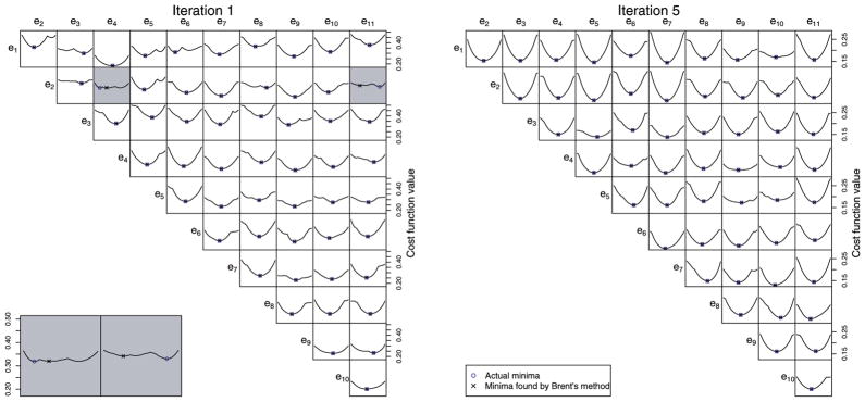
Our optimization procedure is similar to that used in [7]. PCA provides an initial orthonormal basis e, and every possible pair e_i, e_j is rotated together in the 2D plane that they span so that the basis remains orthonormal. Each pair is rotated by the angle θ that minimizes E_var+ λE_loc. The optimal θ is found numerically using Brent’s method [15]. As illustrated in Fig. 2, the global minimum is almost always found at each iteration, even though changes of center point produce slope discontinuities.

Fig. 2.

For each possible pairing of basis vectors among the 10 that account for the highest amounts of shape variation in the ventricle data set, a graph is shown that represents the value of the cost function for all possible angles of rotation of the basis pair in the plane they span. The minimum-cost rotation angle and the rotation angle found by Brent’s method are shown; in almost all cases, these are identical. When they are not (see lower left), it is typically due to a flat cost function where many rotation angles provide nearly the same reduction in cost. These graphs are representative of the graphs for the other data sets.

The pairs are rotated in decreasing order of shape variation accounted for. The set of all e_i, e_j pairs are adjusted repeatedly, and optimization ceases when adjusting them changes the objective function less than a fixed threshold. Between 50 and 150 iterations were required for each experiment discussed below.

4 Results

Below, we compare LoCA to PCA on three data sets, two from brain imaging and one from primate morphology: CCs, lateral ventricles, and colobine monkey crania.¹

LoCA behavior depends strongly on λ, the parameter that modulates the trade-off between conciseness and locality (Fig. 1). For λ = 0, LoCA reduces to PCA. For small λ, LoCA basis vectors accounting for the highest amount of shape variation resemble PCA basis vectors, while the rest of the basis is clearly localized. For larger λ, all LoCA basis vectors are local, and the bases require more basis vectors to account for shape variation in the data. In Figs. 3 and 5, LoCA basis vectors are depicted for the smallest value of λ for which the bases lacked global basis vectors. Reconstruction error for all three data sets is graphed in Table 1, in which we can see that strongly local bases (i.e., higher λ) require more vectors for accurate reconstruction.

Fig. 3.

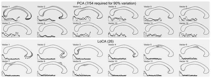
Corpora callosa basis comparison. The first 12 out of 54 basis vectors are shown. LoCA successfully captures the major shape deformations of the genu and splenium in the first four vectors.

Fig. 5.

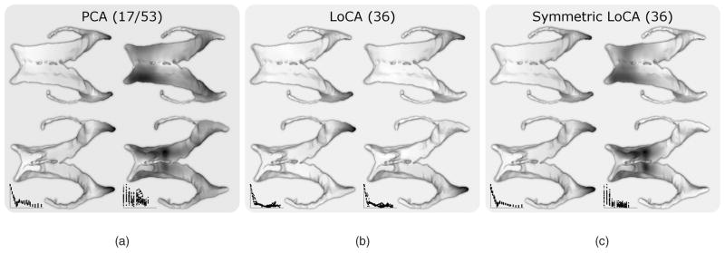
For PCA, LoCA, and Symmetric LoCA, the first two basis vectors in order of reconstruction error are shown from above (left) and below (right). Darker surface points are displaced to a greater degree by the basis vector. For each basis, the number of basis vectors required to account for 90 percent of the ventricular shape variation is given in parentheses. The first PCA vector captures a symmetric change to both occipital horns along with expansion of the left frontal horn, while the second represents a nearly uniform inflation of the entire surface. LoCA finds vectors which affect each side separately while symmetric LoCA affects both simultaneously: its first vector lengthens both occipital horns while its second expands both frontal horns.

TABLE 1.

Reconstruction Error Percentage When Using Only the First k Vectors of the Basis

Corpora callosa reconstruction errors
Basis	1 vector	6	12	18	24
PCA (7/54)	60.57	11.00	4.24	1.98	0.96
LoCA (10)	62.96	13.72	8.42	5.72	3.83
LoCA (15)	72.14	17.38	11.47	7.76	5.32
LoCA (26)	86.60	45.98	24.65	16.87	11.25
Ventricle reconstruction errors
Basis	1 vector	8	16	24	32
PCA (17/53)	63.48	20.72	10.55	5.83	3.16
LoCA (25)	63.66	23.42	14.74	10.02	6.44
LoCA (31)	64.30	27.26	19.45	13.97	9.16
LoCA (36)	80.44	39.60	28.82	20.06	12.81
Symmetric LoCA (25)	63.54	23.76	14.86	10.43	6.98
Symmetric LoCA (31)	63.74	26.17	18.98	13.55	8.99
Symmetric LoCA (36)	65.51	35.28	26.18	18.58	12.20
Crania reconstruction errors
Basis	1 vector	18	36	54	72
PCA (26/135)	67.96	14.63	6.27	2.99	1.37
LoCA (47)	68.20	19.74	12.88	8.39	5.33
LoCA (62)	69.27	29.69	18.90	12.11	7.36
LoCA (76)	79.94	41.52	25.65	16.98	11.08
Symmetric LoCA (45)	70.73	22.95	12.41	7.80	4.81
Symmetric LoCA (61)	76.87	31.38	18.99	11.80	7.34
Symmetric LoCA (78)	89.30	49.48	30.60	19.10	11.84

The numbers in parentheses denote the number of vectors required to capture 90% of the shape variation. For the corpora callosa, these numbers correspond to the different λ settings used in Figure 1. When available, LoCA bases are compared with Symmetric LoCA bases requiring a similar number of vectors.

4.1 Corpora Callosa

The CC data set represents 31 AIDS patients and 19 HIV-seronegative controls (mean age 42.64 ± 11.28 S.D.), who underwent high-resolution magnetic resonance brain scans as part of a previously described study [16]. As part of that study, each scan was rigidly aligned to the ICBM-53 template based on intensity cues, and all scans were then further aligned to each other in a groupwise fashion, based on manual sulcal landmarks. The CC was manually traced on the midsagittal slice of each scan using a reliable and repeatable protocol, partitioned using the Witelson criteria [17], and automatically marked with 103 surface correspondences [18].

We compared the ability of LoCA and PCA to detect what is likely the most firmly established difference in CC morphology between men and women, based on postmortem [17] and imaging-based [19], [20] findings: that women have larger isthmuses (i.e., posterior midbodies). We selected the LoCA and PCA coefficients for the shape components that captured 90 percent of the CC shape variation: the top 7 for PCA and the top 26 for LoCA (see Fig. 3). For each shape component, gender differences in its coefficients were tested in linear statistical models that controlled for other factors known to affect CC morphology: presence of AIDS, handedness, and age. The significance of the gender differences were assessed by F-tests in an ANOVA design.

Among the top 26 LoCA shape components, only components 5 and 9 had coefficients that differed significantly by gender at the p < 0.05 level, indicating thicker superior and inferior aspects of the isthmus in women (component 5: F = 5.44, p = 0.024; component 9: F = 4.24, p = 0.045, p-values uncorrected). This gender difference has been reported extensively (e.g., [17], [19], [20]). Only the first PCA component differed significantly between men and women (F = 5.41, p = 0.024); it represents a complex pattern of elongation, rotation, bending, and twisting of the entire structure. The complexity makes the shape component relatively difficult to interpret in simple anatomical terms. Also, some of the represented modes of CC deformation have not been reported to differ between genders in the literature, so their validity is uncertain.

4.2 Lateral Ventricles

Lateral ventricles were also traced manually in 3D on 54 of the 55 group-aligned scans of healthy and HIV/AIDS patients from a prior study [16]. The boundaries of the frontal, temporal, and occipital horns were traced on each slice based on a reliable, repeatable protocol described previously [21]. Dense one-to-one correspondences between subjects at homologous surface points were established by threading medial curves down the center of each of the frontal, temporal, and occipital horns, and resampling each horn to contain a fixed number of axis-aligned parallel traces [16]. Within each trace, rays were cast outward from the medial curve point toward the ventricular surface every θ radians. Across subjects, 330 correspondences were established between points in analogous traces and analogous θ. Geodesic distances were computed between pairs of resampled surface points, and the distances were used to compute compatibilities. The resampled surface points were the input to the shape parameterization methods.

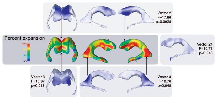
We used PCA and Symmetric LoCA to assess differences in shape component coefficients between AIDS and control groups, and compared the results to differences between these groups that were previously presented using an established radial ventricular mapping approach [16]. The radial mapping approach has been strongly validated and used to characterize ventricular shape variation across a large number of medical covariates [21], [1], [22]. At each surface point, local thickness values were computed by calculating the distance from the surface point to the medial curve; mean thickness values were computed for AIDS and control groups. The ratios of mean local thicknesses between AIDS and control groups were computed and mapped to color values in a 3D rendering of the ventricular surface (Fig. 4). Red regions represent portions of the ventricular surface that were extremely dilated in AIDS patients compared to controls. Coefficients for the top PCA and Symmetric LoCA shape components accounting forn 90 percent of ventricular shape variation were analyzed in statistical models (17 PCA components and 36 LoCA components; the initial vectors in each basis appear in Fig. 5). The LoCA shape components that differed significantly at the p < 0.05 level between groups, in two-tailed t-tests with Bonferroni correction for multiple comparisons, are shown in Fig. 4. The ventricular regions covered by these shape components roughly correspond to the (red) regions that are grossly dilated in AIDS patients on the spatial maps, including the lateral walls, superior ridge, and anterior tip of the frontal horns; the superior and lateral aspects of the occipital horns; and the tips of the temporal horns. The only statistically significant PCA component was the second (Fig. 5, p = 8.59e − 05, t = 26.25), which represents nearly uniform inflation of the entire ventricular surface with no indication that some portions of the surface are more or less dilated in the AIDS group.

Fig. 4.

Differences between AIDS and control groups in ventricular shape as characterized by LoCA and a complementary radial thickness mapping approach. Regions that are extremely dilated in the AIDS group relative to controls are shown in red in the spatial map; LoCA shape components whose coefficients differed significantly between AIDS and control groups are also shown to illustrate the agreement between the methods. The portion of the ventricular surface accounted for by each LoCA shape component is shown in blue. Shown p-values have been Bonferroni-corrected to correct for multiple comparisons. The spatial map was adapted from a similar figure in [16].

4.3 Colobine Monkey Crania

A shape space was built from a set of 238 colobine monkey crania (Subfamily Colobinae, Family Cercopithecidae) representing 17 species (2 of them outgroups). Various primate morphologists collected 45 landmark points on each cranium using a Microscribe 3D digitizer as part of data collection for a long-term project on Old World monkey cranial evolution. Twenty-nine of the landmarks were collected from the dorsal aspect of the cranium and 16 were collected from the ventral aspect (see [23] for details). The landmark sets were rescaled to remove the influence of size differences and aligned using GPA. Since we did not have surface models for each of the specimens, but only the landmarks, we estimated geodesic distance between landmarks by connecting them with a graph representing adjacency on the skull surface, and using distance in the weighted graph to form the compatibility matrix B.

We used a value of λ that produced a completely localized Symmetric LoCA basis, which required 61 components to account for 90 percent of the shape variance (Sym LoCA (61) in Table 1). We then compared branching groups in the evolutionary tree, testing the statistical significance of the PCA and LoCA vectors for discriminating between the two groups. We employed Welch’s two sample t-tests on each sex separately, using Bonferroni correction for multiple comparisons. In each case, we found several statistically significant LoCA components with corrected p-values at or below 0.05.

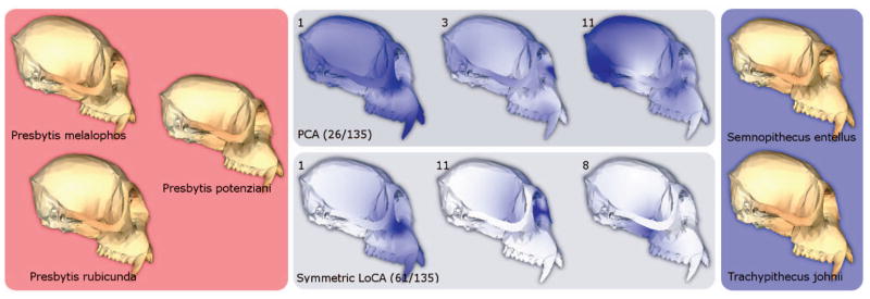
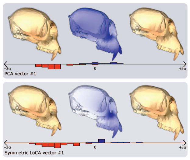
One branch is shown in Fig. 6. We examined the males from two groups, with the first group consisting of Presbytis melalophos, Presbytis potenziani, and Presbytis rubicunda specimens, and the second group consisting of Semnopithecus entellus and Trachypithecus johnii specimens. Each group is visually represented by the average male of each species, alongside the three basis vectors with the lowest p-values for both PCA and LoCA. LoCA vector 1 represents lengthening of the face, which is shorter for the Presbytis group (see Fig. 7). Vector 11 captures the width of the nasal bone, which tends to be narrower for the Presbytis group. Vector 8 shows a deformation of the sphenoid bone, internal to the zygomatic arch (cheekbone) and just behind the tooth row.

Fig. 6.

t-Tests were used to assess differences in PCA and LoCA shape component coefficients between monkey crania drawn from differing branches in an evolutionary tree. Sample crania from the two branches are shown on the left and right. The three PCA vectors and three LoCA vectors with the lowest t-test p-values are depicted visually; the regions of the cranium affected by each vector are shown in dark blue. Each PCA vector represents a complex spatial pattern of shape characteristics, while each LoCA vector focuses on a single localized skull region.

Fig. 7.

The PCA and LoCA vectors with the lowest p-values from Fig. 6 are depicted in more detail: for both basis vectors, crania corresponding to the mean shape component coefficient value over both groups, plus or minus two standard deviations, are shown. Also shown are histograms that give the distributions of coefficient values for the group shown on the left in Fig. 6 (red) and the group shown on the right (blue).

Two of the three most significant PCA vectors shown in Fig. 6 include local deformations identified by significant LoCA vectors. PCA vector 1 affects face length (like LoCA vector 1), and also includes other deformations. Similarly, PCA vector 11 combines the nasal bone deformation of LoCA vector 11 with a complex change to the back of the cranium. The other, PCA vector 3, shows a global change that focuses on the length of the nasal bone, and also deforms the zygomatic arches and affects the cranium’s width. Table 2 shows that both the PCA and LoCA vectors have similar p-values, showing that in this example, the increased locality of the LoCA vectors does not come at the cost of discriminating power.

TABLE 2.

Results of the t-Tests Performed in Fig. 6

	Vector	Eloc	t(41)	p-value
PCA	1	0.322715	10.5302	4.667609e-07
	3	0.175157	6.3989	6.336324e-05
	11	0.223596	−5.7523	1.576577e-04
Symmetric LoCA	1	0.0888693	10.2211	2.324091e-06
	11	0.00808553	7.1989	2.204578e-05
	8	0.0179966	6.763	3.088845e-04

The shown p-values are Bonferroni-corrected. Note that the Symmetric LoCA vectors are both local and find statistically-significant differences between the branching groups.

5 Discussion

The LoCA components spread the shape variation in the ensemble across more significant components than does PCA, with each component optimized for spatial locality. These components isolate the shape variation of specific parts of the object. Because we often understand shape variation in terms of spatially localized object parts, this decomposition is useful in the analysis and interpretation of shape differences between groups. Also, we found that representing the shape of single, rather than multiple, object regions in a single shape parameter helped to prevent the obfuscation of relationships between individual regions and auxiliary variables.

We found that LoCA is broadly applicable to a variety of data sets despite differences in dimension, shape representation, and the density, accuracy, and source of the point-to-point correspondences. This flexibility suggests that it might be applied even more broadly, particularly to articulated forms. The method is also flexible with respect to the definition of compatibility between surface points; the incorporation of symmetry that we used here is just one example. Another appealing possibility would be somehow combining geodesic distance with curvature change, to encourage vectors affecting regions of similar curvature (e.g., the ridges of the ventricles).

In our formulation, pairs of points are more compatible if the geodesic distance between them is lower. Hence, we implicitly encouraged a fixed neighborhood size for our localized basis vectors. It may be more natural to encourage shape basis vectors in which all of the points in a particular surface neighborhood deform in concert, regardless of the size of the neighborhood. Future work will also address the problem of how to construct shape bases whose basis vectors are spatially localized in this scale-invariant fashion.

It is unclear whether we would generate shape parameterizations that are more spatially localized, or more useful for making shape-based inferences, if we dropped the orthogonality constraint from LoCA or added other constraints to the optimization; for example, we could seek shape components that are both spatially localized and statistically independent, as in ICA. Future work will address this variant of our current method.

References

- 1.Carmichael OT, Thompson PM, Dutton RA, Lu A, Lee SE, Lee JY, Kuller LH, Lopez OL, Aizenstein HJ, Meltzer CC, Liu Y, Toga AW, Becker JT. Mapping Ventricular Changes Related to Dementia and Mild Cognitive Impairment in a Large Community-Based Cohort. Proc. IEEE Int’l Symp. Biomedical Imaging; 2006. [Google Scholar]
- 2.Curran-Everett D. Multiple Comparisons: Philosophies and Illustrations. Am J Physiology Regulatory, Integrative and Comparative Physiology. 2000 July;279(1):R1–R8. doi: 10.1152/ajpregu.2000.279.1.R1. [DOI] [PubMed] [Google Scholar]
- 3.Alcantara D, Carmichael O, Delson E, Harcourt-Smith W, Sterner K, Frost S, Dutton R, Thompson P, Aizenstein H, Lopez O, Becker J, Amenta N. Localized Components Analysis. Proc Information Processing in Medical Imaging. 2007:519–531. doi: 10.1007/978-3-540-73273-0_43. [DOI] [PMC free article] [PubMed] [Google Scholar]
- 4.Cootes TF, Hill A, Taylor CJ, Haslam J. The Use of Active Shape Models for Locating Structures in Medical Images. Image and Vision Computing. 1994 July;12(6):355–366. [Google Scholar]
- 5.Bookstein FL. Morphometric Tools for Landmark Data: Geometry and Biology. Cambridge Univ. Press; 1991. [Google Scholar]
- 6.Allen B, Curless B, Popovic Z. The Space of Human Body Shapes: Reconstruction and Parameterization from Range Scans. Proc ACM SIGGRAPH. 2003:587–594. [Google Scholar]
- 7.Chennubhotla C, Jepson A. Sparse PCA: Extracting Multi-Scale Structure from Data. Proc Int’l Conf Computer Vision. 2001:641–647. [Google Scholar]
- 8.Zou H, Hastie T, Tibshirani R. Sparse Principal Component Analysis. J Computational and Graphical Statistics. 2006 June;15(2):265–286. [Google Scholar]
- 9.Sjöstrand K, Stegmann MB, Larsen R. Sparse Principal Component Analysis in Medical Shape Modeling. Proc. SPIE Int’l Conf. Medical Imaging: Image Processing; 2006. [Google Scholar]
- 10.Stegmann MB, Sjöstrand K, Larsen R. Sparse Modeling of Landmark and Texture Variability Using the Orthomax Criterion. Proc. SPIE Int’l Conf. Medical Imaging: Image Processing; 2006. [Google Scholar]
- 11.Üzümcü M, Frangi A, Sonka M, Reiber J, Lelieveldt B. ICA vs. PCA Active Appearance Models: Application to Cardiac MR Segmentation. Proc. Int’l Conf. Medical Image Computing and Computer-Assisted Intervention; 2003. pp. 451–458. [Google Scholar]
- 12.Ballester MAG, Linguraru MG, Aguirre MR, Ayache N. On the Adequacy of Principal Factor Analysis for the Study of Shape Variability. Proc. SPIE Int’l Conf. Medical Imaging: Image Processing; 2005. [Google Scholar]
- 13.Vermaak J, Perez P. Constrained Subspace Modeling. Proc. Conf. Computer Vision and Pattern Recognition; June 2003. [Google Scholar]
- 14.Pizer S, Fritsch D, Yushkevich P, Johnson V, Chaney E, Gerig G. Segmentation, Registration, and Measurement of Shape Variation via Image Object Shape. IEEE Trans Medical Imaging. 1999 Oct;18(10):851–865. doi: 10.1109/42.811263. [DOI] [PubMed] [Google Scholar]
- 15.Press W, Teukolsky S, Vetterling WT, Flannery B. Numerical Recipes in C. 2. Cambridge Univ. Press; 1992. [Google Scholar]
- 16.Thompson P, Dutton R, Hayashi K, Lu A, Lee S, Lee J, Lopez O, Aizenstein H, Toga A, Becker J. 3D Mapping of Ventricular and Corpus Callosum Abnormalities in HIV/AIDS. NeuroImage. 2006 May;31(1):12–23. doi: 10.1016/j.neuroimage.2005.11.043. [DOI] [PubMed] [Google Scholar]
- 17.Witelson S. Hand and Sex Differences in the Isthmus and Body of the Corpus Callosum: A Postmortem Morphological Study. Brain. 1989;112:799–835. doi: 10.1093/brain/112.3.799. [DOI] [PubMed] [Google Scholar]
- 18.Ghosh D, Amenta N. Technical Report CSE-2007-6. Dept. of Computer Science, Univ. of California; Davis: 2007. Landmark Transfer Using Deformable Models. [Google Scholar]
- 19.Habib M, Gayraud D, Oliva A, Regis J, Salamon G, Khalil R. Effects of Handedness and Sex on the Morphology of the Corpus Callosum: A Study with Brain Magnetic Resonance Imaging. Brain and Cognition. 1991 May;16(1):41–61. doi: 10.1016/0278-2626(91)90084-l. [DOI] [PubMed] [Google Scholar]
- 20.Steinmetz H, Jancke L, Kleinschmidt A, Schlaug G, Volkmann J, Huang Y. Sex but No Hand Difference in the Isthmus of the Corpus Callosum. Neurology. 1992 Apr;42(4):749–752. doi: 10.1212/wnl.42.4.749. [DOI] [PubMed] [Google Scholar]
- 21.Narr KL, Thompson PM, Sharma T, Moussai J, Blanton R, Anvar B, Edris A, Krupp R, Rayman J, Khaledy M, Toga AW. Three-Dimensional Mapping of Temporo-Limbic Regions and the Lateral Ventricles in Schizophrenia: Gender Effects. Biological Psychiatry. 2001;50:84–97. doi: 10.1016/s0006-3223(00)01120-3. [DOI] [PubMed] [Google Scholar]
- 22.Thompson P, Hayashi K, de Zubicaray G, Janke A, Rose S, Semple J, Hong M, Herman D, Gravano D, Doddrell D, Toga A. Mapping Hippocampal and Ventricular Change in Alzheimer’s Disease. Neuro-Image. 2004 Aug;22(4):1754–1766. doi: 10.1016/j.neuroimage.2004.03.040. [DOI] [PubMed] [Google Scholar]
- 23.Frost SR, Marcus LF, Bookstein FL, Reddy DP, Delson E. Cranial Allometry, Phylogeography, and Systematics of Large-Bodied Papionins (Primates: Cercopithecinae) Inferred from Geometric Morphometric Analysis of Landmark Data. The Antatomical Record Part A. 2003;275A:1048–1072. doi: 10.1002/ar.a.10112. [DOI] [PubMed] [Google Scholar]