Continuous Glucose Monitoring: Real-Time Algorithms for Calibration, Filtering, and Alarms

Abstract

Algorithms for real-time use in continuous glucose monitors are reviewed, including calibration, filtering of noisy signals, glucose predictions for hypoglycemic and hyperglycemic alarms, compensation for capillary blood glucose to sensor time lags, and fault detection for sensor degradation and dropouts. A tutorial on Kalman filtering for real-time estimation, prediction, and lag compensation is presented and demonstrated via simulation examples. A limited number of fault detection methods for signal degradation and dropout have been published, making that an important area for future work.

Introduction

The ability of individuals with type 1 diabetes to monitor blood glucose levels has improved tremendously over the past four decades. The use of self-monitoring of blood glucose (SMBG) meters certainly has led to a tremendous improvement in glucose monitoring compared to urine strips. Continuous glucose monitoring (CGM) has the potential to further reduce mean glucose levels while avoiding the risk of hypoglycemia. It is also a necessary component of a closed-loop artificial pancreas.

A goal of this article is to review mathematical algorithms that have been proposed for use in CGM technology. Because our focus is on minimally invasive, subcutaneous sensors, we do not include an analysis of algorithms for noninvasive glucose sensors. Our primary interest is in algorithms proposed for hypoglycemic and hyperglycemic alarms, but a number of other important algorithms must be used for a successful alarm strategy. Thus, algorithms used for calibration, filtering raw current signals, handling of signal artifacts, compensation of the lag between blood and interstitial fluid, and hypo- and hyperglycemic alarms are discussed. Closed-loop control algorithms are not discussed; reviews of algorithms for a closed-loop artificial pancreas are discussed elsewhere.^1–4

Background

There have been a number of reviews of sensor and related technologies for continuous glucose monitoring for diabetes applications. Klonoff^5,6 provided reviews of the state of continuous glucose monitoring technology, circa 2004. At that time, the only real-time device approved by the Food and Drug Administration (FDA) for the U.S. market was the GlucoWatch G2 Biographer. An article by the JDRF CGM Study Group⁷ summarized the design and methods used to test the three continuous glucose monitoring systems (CGMS) currently approved by the U.S. FDA for the U.S. market.

Skyler⁸ provided a comprehensive history of CGM development as an editorial introduction to a special issue on CGM. A tutorial overview of current CGM technology was provided by Kerr and Fayers,⁹ while Oliver and colleagues¹⁰ provided a more comprehensive review of noninvasive glucose sensor technology. Cox¹¹ provided a head-to-head comparison of the currently available CGM systems.

A CGM Standards report¹² provided consensus guidelines on how CGM data should be presented and compared between CGM devices, and different glucose measurement methods. Important topics included the evaluation of threshold alarms, calibration, and sensor and physiological lag times. Lodwig and Heinemann¹³ discussed a number of important topics related to CGM calibration. Hayter and associates¹⁴ proposed performance standards of CGM devices, including methods of data analysis and acceptable rates of false alarms for hypoglycemia.

Calibration

Although an objective in diabetes management is to control blood glucose to near euglycemic levels, minimally invasive continuous glucose sensors output a signal that is proportional to the interstitial glucose value. A calibration algorithm is used to convert the raw sensor signal, typically in nanoamps, to a blood glucose estimate (milligrams per deciliter in the United States). In most cases, a simple linear equation is used

$$y=mx+b,$$ (1)

where x is the independent variable (usually reference blood glucose) and y is the dependent variable (usually the sensor current). If the y intercept is assumed to be known (usually b = 0), then a one-point calibration can be used to find the sensor sensitivity (or slope, m), where

$$m=\left(y-b\right)/x$$ (2)

and only one sensor signal (y) – blood glucose (x) pair is used.

A two-point calibration is based on the two sensor/glucose pairs, where the subscripts 1 and 2 represent the first and second calibration data points, respectively,

$$\begin{array}{c}{y}_1=m{x}_1+b\\ y_2=m{x}_2+b\end{array}.$$ (3)

The slope and intercept are estimated from

$$\begin{array}{cc}m=\frac{\left(y_2-y_1\right)}{\left(x_2-x_1\right)}& b=y_2-m{x}_2\end{array}.$$ (4)

Further, when multiple data points are available, then linear regression can be used to fit slope and intercept to data. The assumption is that there is uncertainty in the output measurement, and the equation has the form¹⁵

$$y_i=m{x}_i+b+e_i,$$ (5)

where the subscript i represents the ith data point. Standard linear regression techniques find the slope (m) and intercept (b) that minimize the sum of the squares of the errors (differences between measurements and model predictions, where ${\hat{y}}_i=m{x}_i+b$) over N data points

$$\underset{m,b}{\min }{\displaystyle \mathbf{\sum }_{i=1}^N{e}_i^2}=\underset{m,b}{\min }{\displaystyle \mathbf{\sum }_{i=1}^N{\left(y_i-{\hat{y}}_i\right)}^2.}$$ (6)

Once the sensor is calibrated, the estimated glucose concentration is obtained from the sensor current from

$$\hat{x}=\frac{\left(y-b\right)}{m}.$$ (7)

The correlation coefficient is a measure of the quality of the model fit; if the correlation coefficient is too low, the calibration may be deemed unacceptable, requiring additional reference glucose measurements, as discussed in the patent by Goode and colleagues.¹⁶ Further, the patent by Feldman and McGarraugh¹⁷ discussed criteria for calibration acceptance.

Linear regression analysis assumes that the independent variable is known and that the dependent variable is uncertain. If Yellow Springs Instruments glucose data are used for sensor calibration, this may be a good assumption, but standard reference glucose test meters have substantial error.¹⁸ Panteleon and colleagues¹⁹ obtained better sensor calibration results (lower mean average deviation of blood and subcutaneous glucose) when the raw glucose current signal is used as the independent variable in linear regression analysis

$$x_i=m^{\prime }{y}_i+b^{\prime }+e_i,$$ (8)

where the parameters m′ and b′ are found by minimizing the objective function (where ${\hat{x}}_i=m^{\prime }{y}_i+b^{\prime }$)

$$\underset{m^{\prime },b^{\prime }}{\min }{\displaystyle \mathbf{\sum }_{i=1}^N{e}_i^2}=\underset{m^{\prime },b^{\prime }}{\min }{\displaystyle \mathbf{\sum }_{i=1}^N{\left(x_i-{\hat{x}}_i\right)}^2.}$$ (9)

Deming regression is an “error in variables” technique that assumes uncertainty in both independent and dependent variables. Panteleon and associates¹⁹ noted that the two different calibration procedures (reference blood glucose vs sensor current signal as independent variables) provide bounds on the results that would be obtained using Deming regression.

The findings by Panteleon and colleagues¹⁹ were also demonstrated by Choleau and associates,²⁰ who showed, via simulation, that errors in the reference glucose and continuous sensor can cause the slope and intercept to be correlated. In a related paper, Choleau and colleagues²¹ used error grid analysis²² to show that the one-point calibration method is superior to the two-point calibration, based on rat studies. They also found that two one-point calibrations yielded nearly as good calibration as three one-point calibrations. The use of multiple sensor–glucose data pairs and linear regression was not discussed, however.

Usually the time lag between the capillary blood glucose and the raw sensor signal is neglected by the calibration algorithm, so it is important to calibrate when the sensor glucose signal is relatively constant, assuring that the interstitial fluid glucose concentration is in equilibrium with the capillary blood. Aussedat and colleagues²³ proposed an automated calibration request that detects a “plateau” when the sensor signal has not changed by more than 1% over a 4-minute window and when the sensor current for the second calibration point differs from the first by 2 nA or greater. Studies were conducted in rats.

Errors in glucose meter reading, in addition to lags between blood and interstitial glucose, make it necessary that the two reference blood glucose values differ significantly when using a two-point calibration. King and colleagues²⁴ showed how sensor performance varies as a function of the difference in the reference blood glucose values used for calibration, suggesting that they differ by >30 mg/dl. Indeed, they found that using two values separated by 40 mg/dl led to nearly the same performance as a retrospective calibration over a large number of glucose values.

The DirecNet Study Group²⁵ evaluated factors affecting calibration of the Medtronic CGMS. Sensor accuracy was improved slightly with more calibrations per day; also, accuracy was degraded when calibrating with glucose rates of change ±1.5 mg/dl/min. Another finding was that overnight sensor accuracy was improved if only overnight calibrations were used; it is suggested that a separate calibration algorithm be used for overnight reading. Finally, it should be noted that the calibrations were retrospective, but the authors suggested that similar improvements would be expected from prospective calibration.

Discussion

Basing glucose sensor calibration on SMBG meter readings remains a major weakness of CGM technology. Errors in the reference glucose can lead to substantial bias in the calibrated CGM signal, having an effect for much of a 24-hour period, depending on the frequency of calibration. It is difficult to incorporate SMBG uncertainty into the calibration, based on statistical techniques, because of the small set of data (only a few finger stick measurements each day).

Filtering Raw Sensor Signals

Virtually all sensors have signal noise that must be “filtered” before the signals can be used by any computational algorithm or real-time display. Continuous glucose sensors have analog filters to smooth the current output to the analog-to-digital (A to D) converter, but even these sensor signals are noisy and must be filtered. It is particularly important to use filtered glucose values for applications based on the rate of change of glucose, particularly as these computations are based on differences in successive measurements. This section focuses on digital filtering and does not cover the analog filters that are in the sensor hardware.

Median Filters

A median filter takes the median value of a window of N past glucose values

$${\hat{y}}_k=median\left(y_k,y_{k-1},\dots ,y_{k-N+1}\right)$$ (10)

and has the advantage of discarding the effect of anomalous values due to “spikes” in the signal. Poitout and colleagues²⁶ used a median filter based on the median of the past five sensor current values.

Finite and Infinite Impulse Response Filters

The most common filtering algorithms are finite and infinite impulse response filters. A finite impulse response (FIR) filter has the form

$${\hat{y}}_k=a_0{y}_k+a_1{y}_{k-1}+\cdots +a_M{y}_{k-M},$$ (11)

where y represents the measured glucose value and $\hat{y}$ the filtered value. A simple example is a moving average filter, with all data points in the data window weighted equally. For example, with a window of five samples, the following fifth-order filter

$${\hat{y}}_k=0.2y_k+0.2y_{k-1}+0.2y_{k-2}+0.2y_{k-3}+0.2y_{k-4}$$ (12)

would create an effective delay of the order of 2.5 sample times. Panteleon and colleagues¹⁹ cited use of a seventh-order FIR filter for signals sampled at a 1-minute interval. Medtronic patents^27,28 show raw signals being obtained at 10-second intervals. At the end of each 1-minute interval, the lowest and highest values are removed, and the remaining four are averaged to obtain the 1-minute average. Similarly, every 5-minute interval removes the lowest and highest 1-minute averages and averages the remaining three data points for the 5-minute average. Removing the highest and lowest values has a similar effect to median filtering. “Clipping limits” can be applied to limit the rate of change of either the raw signal or calibrated glucose values. Keenan and associates²⁹ noted that the Medtronic CGMS Gold and Guardian RT have different filtering algorithms.

An infinite impulse response (IIR) filter has the form

$${\hat{y}}_k=-a_1{\hat{y}}_{k-1}-\cdots -a_N{\hat{y}}_{k-N}+b_0{y}_k+b_1{y}_{k-1}+\cdots +b_M{y}_{k-M},$$ (13)

where the current filtered value of the output is a function of N previously filtered values, as well as current and M previous measurements. A patent assigned to Dexcom¹⁶ suggests the use of IIR filters for raw signal filtering, with an example of N = 3 and M = 3. It should be noted that filters can also be applied to the derivative of the glucose (or its change between two successive measurements); this approach is cited in the Medtronic patent of Steil and Rebrin³⁰ and is particularly useful as part of a closed-loop algorithm based on the rate of change of glucose.

Optimal Estimation Theory

The optimal estimation theory approach of Knobbe and Buckingham³¹ and Knobbe and associates,³² based on use of a continuous-discrete extended Kalman filter, explicitly accounts for both sensor noise and uncertainty in reference glucose (finger stick) measurements. Based on use of a discrete dual-rate Kalman filter, a similar approach was used by Bequette and colleagues³³ and Kuure-Kinsey colleagues.³⁴ The next section provides a tutorial overview of Kalman filtering.

Glucose Estimation and Prediction for Hypoglycemic and/or Hyperglycemic Alarms

One of the major motivations for the use of continuous glucose monitoring is to detect or predict the onset of hypoglycemia. Heise and colleagues³⁵ provided an overview of requirements for a successful alarm system based on CGM. CGM alarms can be based on either threshold (limit exceeded by the current glucose measurement) or projected (a limit is expected to be exceeded at some point in the future, usually 10–45 minutes) alarms. Currently, Dexcom sensors use a threshold alarm, whereas the Medtronic Guardian RT and Abbott Navigator systems have both a threshold and a projected alarm.³⁶

Linear Regression and Linear-in-Time Projections

Perhaps the most intuitive (and most common) method of predicting glucose values is to perform linear regression using a “window” of recent glucose measurements (filtered, raw, or estimates of glucose) and assuming that the slope remains constant into the future. As an example, consider the simulated set of glucose sensor measurements shown in Figure 1, where t = 0 is the current time. Standard linear regression analysis yields not only an estimate of the slope and intercept parameters but confidence intervals as well. These confidence intervals can also be used in the future prediction, yielding a region of possible glucose values, as shown 30 minutes into the future in Figure 1.

Figure 1.

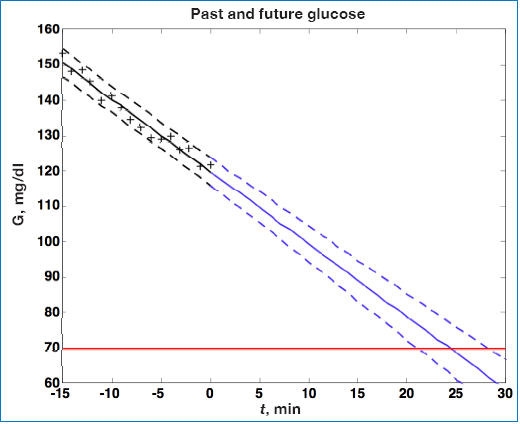
Continuous glucose (G) measurements are plotted as (+) from t = −15 to t = 0 minute. Linear regression is used to fit data to the solid line, retrospectively, from t = −15 to 0 minute. Dashed lines represent ±95% confidence intervals. Note that confidence intervals grow for predictions from t = 0 to t = 30 minutes into the future.

The equation used for linear regression is a first-order “polynomial-in-time” model

$$y_k=\alpha t_k+\beta ,$$ (14)

where the subscript k represents the kth sample time, α is the estimated slope, and β is the estimated intercept.

Noujaim and colleagues³⁷ performed simulation studies, similar to that shown in Figure 1, for a glucose rate of change of −5 mg/dl/min. Based on metrics proposed in their paper, they showed that achieving false negative and false positive ratios of <5 and <10%, respectively, would require a CGM to have an mean absolute relative deviation of ≤7.5%. Brauker³⁸ suggested a “zone” of future glucose possibilities, which is the same idea as that shown in Figure 1.

The Abbott FreeStyle Navigator continuous glucose monitoring (FSN-CGM) system has both threshold and projected alarms. McGarrough and Bergenstal³⁹ presented in-clinic and in-home results for the FSN-CGM. For projected alarms, a window of 15 minutes of sensor data is used to estimate the rate of change of glucose and its uncertainty. If the uncertainty is below a certain value and the projected glucose is below a threshold of 85 mg/dl within 10, 20, or 30 minutes, for low, medium, and high sensitivity alarms, respectively (as selected by the patient), an alarm is activated.

Another linear projection method (used in the voting method presented by Cameron and colleagues⁴⁰ and Dassau and colleagues⁴¹ and the pump shutoff studies of Buckingham and associates⁴²) is to consider the end points of a data window

$${\text{rate}}_k=\frac{y_k-y_{k-N}}{N\Delta t}$$ (15)

and find the mean squared error of the rate based on single sample times over the same interval

$${\text{MSErate}}_k={\displaystyle \mathbf{\sum }_{i=0}^{N-1}{\left(\left(\frac{y_{k-i}-y_{k-i-1}}{\Delta t}\right)-{\text{rate}}_k\right)}^2.}$$ (16)

The standard deviation of the rate estimate is

$$\sigma \left({\text{rate}}_k\right)\text{=}\frac{\sqrt{{\text{MSErate}}_k}}{N-1}.$$ (17)

Further, this can be scaled by the absolute value of the rate of change

$${\text{unc}}_k=\frac{\sigma \left({\text{rate}}_k\right)}{\left|{\text{rate}}_k\right|}$$ (18)

and if the scaled uncertainty is greater than some threshold value, the prediction is not accepted.

Choleau and associates⁴³ used a window of 10 minutes, with a sensor sample time of 0.5 minute, and linear regression to estimate the slope (glucose rate of change) and to project the glucose concentration 20 minutes into the future. If the projected glucose is 70 mg/dl or less, the alarm is triggered. Experimental data are presented based on rat studies.

Cameron and colleagues⁴⁴ developed a similar approach in their development of a statistical-based hypoglycemic alarm. Their technique, however, involves the consideration of multiple window lengths of past data for multiple linear regressions. In addition, they considered several different prediction horizons. A similar approach is proposed in the patent by Dunn and colleagues,⁴⁵ who suggested a “mixture of experts” based on the superposition of multiple linear regressions.

The previous methods require that filtered glucose concentrations be used to develop the models for future projections. The theory of optimal estimation and prediction, however, combines signal filtering with model-based estimation and is discussed in the following subsection.

Optimal Estimation and Prediction Theory

Palerm and colleagues⁴⁶ developed a Kalman filter-based approach to estimate the future values of blood glucose. They explored the effect of sample time, hypoglycemic threshold, and prediction horizon on the sensitivity and specificity of the predictions and discussed how the optimal estimators can be tuned to trade-off the false alarm rate with the rate of missed hypoglycemic episodes; this suggests that an individual can tune the alarm depending on their personal risk for hypoglycemia. Palerm and Bequette⁴⁷ validated this approach to data obtained from hypoglycemic clamp studies. Buckingham³⁶ also recommended that the hypoglycemic alarm threshold be tunable to meet an individual's particular needs.

The underlying model is

$$\begin{array}{l}{x}_{k+1}=\mathbf{\Phi }{x}_k+{\mathbf{\Gamma }}^w{w}_k\hfill \\ y_k=C{x}_k+v_k\hfill \end{array},$$ (19)

where x is a vector of states and y is measured output, w_k is process noise (covariance Q), and υ_k is measurement noise (covariance R). If it is assumed that process noise drives the first derivative of glucose with time, then the following relationships result

$$\begin{array}{l}{g}_{k+1}=g_k+d_k\hfill \\ d_{k+1}=d_k+w_k,\hfill \\ y_k=g_k+{\upsilon }_k\hfill \end{array}$$ (20)

where g and d represent the glucose and the change in glucose from step to step, respectively. The state space model corresponding to Equation (20) is

$$\begin{array}{llll}\underset{x_{k+1}}{\underbrace{{\left[\begin{array}{c}g\\ d\end{array}\right]}_{k+1}}}=\underset{\mathbf{\Phi }}{\underbrace{\left[\begin{array}{cc}1& 1\\ 0& 1\end{array}\right]}}\underset{x_k}{\underbrace{{\left[\begin{array}{c}g\\ d\end{array}\right]}_k}}+\underset{{\mathbf{\Gamma }}^w}{\underbrace{\left[\begin{array}{c}0\\ 1\end{array}\right]}}{w}_k\hfill & \hfill & \hfill & \hfill \\ y_k=\underset{C}{\underbrace{\left[\begin{array}{cc}1& 0\end{array}\right]}}\underset{x_k}{\underbrace{{\left[\begin{array}{c}g\\ d\end{array}\right]}_k}}+{\upsilon }_k\hfill & \hfill & \hfill & .\hfill \end{array}$$ (21)

Process and measurement noise are considered stochastic processes, and the process noise covariance (Q) is known only approximately and is often used as a tuning parameter. The states are estimated using predictor–corrector equations of the form:

$$\begin{array}{cc}{\hat{x}}_{k|k-1}=\mathbf{\Phi }{\hat{x}}_{k-1|k-1}& \text{predictor\hspace{0.17em}}\left(\text{time\hspace{0.17em}update}\right)\end{array}$$ (22)

and the glucose sensor measurement is used to update the state estimate

$$\begin{array}{l}{\hat{x}}_{k|k}={\hat{x}}_{k|k-1}+L_k\left(y_k-C{\hat{x}}_{k|k-1}\right)\\ \text{\hspace{1em}\hspace{1em}\hspace{1em}\hspace{1em}\hspace{1em}\hspace{1em}\hspace{1em}corrector\hspace{0.17em}}\left(\text{measurement\hspace{0.17em}update}\right)\end{array}$$ (23)

where $\hat{x}$ represents an estimate of the states and the subscript k|k – 1 means the estimate at step k is based on measurements up (and including) step k – 1. Note that a model is used to propagate the state estimate from the previous time step (k – 1) to the current time step (k). The measurement at the current time step is then used to update the state estimate based on Kalman gain (L_k).

The state estimate covariance is determined by solving

$$P_k=\mathbf{\Phi }{P}_{k-1}{\mathbf{\Phi }}^T+{\mathbf{\Gamma }}^{w}Q{\mathbf{\Gamma }}^{wT}-\mathbf{\Phi }{P}_{k-1}{C}^T{\left(C{P}_{k-1}{C}^T+R\right)}^{-1}C{P}_{k-1}{\mathbf{\Phi }}^T,$$ (24)

where the first two terms on the right-hand side of the equals sign represent the propagation of state covariance and process noise, while the third term represents a correction due to the measurement update (including the effect of measurement noise)

$$L_k=P_k{C}^T{\left(C{P}_k{C}^T+R\right)}^{-1}.$$ (25)

Essentially, the Kalman filter provides a trade-off between the likelihood that a change in a sensor reading is due to a real effect (such as capillary blood glucose changing) and sensor noise. For more background on Kalman filtering and optimal estimation, see Stengel.⁴⁸

Future glucose predictions from the most recent measurement at time step k to step k + j are given by

$${\hat{x}}_{k+j|k}={\mathbf{\Phi }}^j{\hat{x}}_{k|k}.$$ (26)

For the two-state model in Equation (21), this is equivalent to assuming that the rate of change of glucose is constant in the future. That is, for the jth future time step

$${\hat{g}}_{k+j|k}={\hat{g}}_{k|k}+j{\hat{d}}_{k|k},$$ (27)

where ${\hat{d}}_{k|k}$ is the estimated change in glucose from step k – 1 to step k (the current measurement). Uncertainty in the future grows as [Equation (24) without the measurement feedback term]

$$P_k=\mathbf{\Phi }{P}_{k-1}{\mathbf{\Phi }}^T+{\mathbf{\Gamma }}^{w}Q{\mathbf{\Gamma }}^{wT}.$$ (28)

For this problem, the confidence interval grows with each step not followed by a measurement update as there are two “integrators” in the glucose model; this behavior is demonstrated in the simulations that follow.

Consider the simulated noise sequence presented in Figure 1 where Kalman filtering is used to obtain glucose and rate of change of glucose, in real time, despite substantial measurement noise. The state vector estimate is initialized with the measured glucose at t = −15 minutes, with an assumed rate of change of 0 mg/dl/min. Figure 2 displays real-time estimates of glucose (top) and its rate of change (bottom) along with the uncertainty bounds of each. Although the actual rate of change was −2 mg/dl/min, the Kalman filter converges to this value within 15 minutes. Figure 3 shows predicted glucose values based on measurements available until t = 0 minute. Because of the uncertainty about future rates of change, confidence intervals of the glucose predictions increase each step into the future; simulation details are provided in the Appendix. The increase in uncertainty bounds in Figure 3 (based on Kalman filtering), compared to Figure 1 (based on linear regression analysis), is an artifact of assumptions used in the simulation. The smaller linear regression confidence bounds are due to the fact that the real underlying signal has a constant slope, while the Kalman filter “recognizes” that the slope may change in the future.

Figure 2.

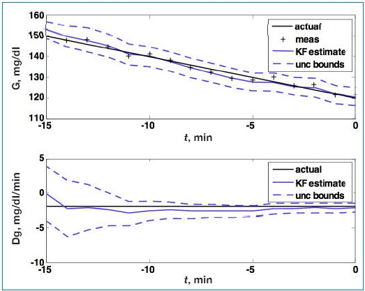
Glucose (G; top) and rate of change of glucose (Dg; bottom). Actual (black), Kalman filter (KF) estimate (blue), and uncertainty (unc) bounds (- - -). The Kalman filter was initialized at t = −15 minutes, with uncertainty in the glucose and rate-of-change states. The estimated error variance improves with measurement (meas) updates. Q = 0.01, R = 4.

Figure 3.

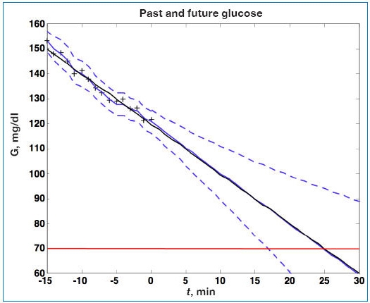
Actual glucose (G; black), measured (+), estimated (blue), and uncertainty bounds (- -). The Kalman filter was initialized at t = −15 minutes. After t = 0 the estimated error variance grows as there are no measurements to improve the estimates.

Facchinetti and colleagues⁴⁹ presented a two-state Kalman filter that has identical behavior to our two-state model shown in Equation (21). Their integrated random walk model is presented in the form

$$\begin{array}{l}{g}_{k+1}=2g_k-g_{k-1}+w_k\hfill \\ y_k=g_k+{\upsilon }_k\hfill \end{array},$$ (29)

which has the state space form

$$\begin{array}{llll}\underset{x_{k+1}}{\underbrace{{\left[\begin{array}{c}{x}_1\\ x_2\end{array}\right]}_{k+1}}}=\underset{\mathbf{\Phi }}{\underbrace{\left[\begin{array}{cc}2& -1\\ 1& 0\end{array}\right]}}\underset{x_k}{\underbrace{{\left[\begin{array}{c}{x}_1\\ x_2\end{array}\right]}_k}}+\underset{{\mathbf{\Gamma }}^w}{\underbrace{\left[\begin{array}{c}1\\ 0\end{array}\right]}}{w}_k\hfill & \hfill & \hfill & \hfill \\ y_k=\underset{C}{\underbrace{\left[\begin{array}{cc}1& 0\end{array}\right]}}\underset{x_k}{\underbrace{{\left[\begin{array}{c}{x}_1\\ x_2\end{array}\right]}_k}}+{\upsilon }_k\hfill & \hfill & \hfill & ,\hfill \end{array}$$ (30)

where the first state is the glucose and the second state is the value of glucose at the previous time step. Although the performance of the resulting Kalman filter is equivalent to results shown in Figures 2 and 3, we feel that our formulation is more natural, as our second state is the rate of change of glucose, which is applied directly to future predictions. Facchinetti and associates⁴⁹ developed a nice procedure for tuning the Kalman filter based on data from individual subjects.

The Kalman filter estimates shown in Figures 2 and 3 are based on a second-order (two-state) model. However, if it is assumed that process noise drives the second derivative of glucose with time, the following third-order (three-state) model can be used:

$$\begin{array}{l}\mathbf{\Phi }=\left[\begin{array}{ccc}1& 1& 0\\ 0& 1& 1\\ 0& 0& 1\end{array}\right],{\mathbf{\Gamma }}^w=\left[\begin{array}{c}0\\ 0\\ 1\end{array}\right],\hfill \\ C=\left[\begin{array}{ccc}1& 0& 0\end{array}\right],x=\left[\begin{array}{c}g\\ d\\ f\end{array}\right],y=G,\hfill \end{array}$$ (31)

where g, d, and f represent glucose, rate of change of glucose, and the second derivative of glucose with respect to time, respectively. The advantage of the three-state model is that it captures dynamics near the maximum (peak) and minimum (valley) values of glucose. While the three-state model yields better estimates for previous and current glucose estimates, Palerm and Bequette⁴⁷ found that the assumption of a constant first derivative (two state) for future predictions led to better performance for multistep-ahead predictions on clinical data than assuming a constant second derivative (three state).

Autoregressive (AR) Model Prediction

Bremer and Gough⁵⁰ applied AR models to blood glucose data available at 10-minute sample times and compared predictions for 10, 20, and 30 minutes ahead. An AR model has the form

$$y_k={\displaystyle \mathbf{\sum }_{i=1}^n{a}_i{y}_{k-i}}+w_k,$$ (32)

where y is the glucose value, w is a white noise sequence, and there are n coefficients, a_i (i.e., the model is nth order). An autoregressive moving average model has a more general form with n a_i coefficients and m c_i coefficients

$$y_k={\displaystyle \mathbf{\sum }_{i=1}^n{a}_i{y}_{k-i}}+{\displaystyle \mathbf{\sum }_{i=0}^{m-1}{c}_i{w}_{k-i}}.$$ (33)

Reifman and colleagues⁵¹ studied a sensor with a sample time of 1 minute and used 2000 data points (2000 minutes) to “train” a 10th-order AR model (n = 10); that is, they fit the 10 model parameters to data. The performance of this model is based on the ability to match 4000 additional minutes of data. They found that a prediction horizon of 30 minutes yields a root mean square error of 22 mg/dl, with a prediction delay. In order to reduce the prediction delay, Gani and colleagues⁵² used a smoothing procedure and regularization to minimize changes in the glucose first derivatives. This approach, with a 30th-order model, reduces the prediction lag compared to the results of Reifman and associates.⁵¹

Sparacino and colleagues⁵³ used an adaptive first-order model, where the parameter is updated at each time step to estimate future glucose values and compared this with a first-order “polynomial-in-time” approach. Zanderigo and associates assessed the accuracy using a continuous glucose error-grid analysis. Sparacino and colleagues provided a tutorial overview of algorithms for continuous glucose monitoring and glucose prediction for use in hypo/hyperglycemic alarms. They noted that a limitation to the approach of Reifman and colleagues⁵¹ is the substantial amount of training data required for estimation of a large number of parameters in a fixed-parameter formulation. Gani and colleagues addressed this criticism by showing that a model could be produced once for a particular individual and then used on other individuals.

Eren-Oruklu and associates^57,58 developed a more general approach, including real-time adaptation of parameters, and found that the best model is second order, with the form

$$y_k=a_1{y}_{k-1}+a_2{y}_{k-1}+w_k+c_1{w}_{k-1},$$ (34)

while Sparacino and colleagues⁵³ used a first-order model

$$y_k=a_1{y}_{k-1}+w_k.$$ (35)

In these studies, model coefficients are estimated recursively, using weighted least squares, where data further in the past have less of an impact than more recent data. That is, the parameters are found to solve the optimization problem

$$\min {\displaystyle \mathbf{\sum }_{i=0}^{N-1}{\mu }^i}{\left(y_{k-i}-{\hat{y}}_{k-i}\right)}^2,$$ (36)

where μ is a “forgetting factor,” with values between 0 and 1. The forgetting factor^57,58 is adapted based on a change detection method that reduces μ during periods of rapid glucose change. Further, statistical process monitoring techniques⁵⁸ (control charts) are used to activate hypoglycemic alarms.

Combined Methods

Recognizing that each of the hypoglycemic prediction methods has strengths and weaknesses, a voting method^40,41 was used to determine when hypoglycemia is likely to occur. The algorithms employed include Kalman filtering,⁴⁷ hybrid adaptive IIR, linear polynomial in time, statistical hypoglycemia prediction,⁴⁴ and a numerical logical algo-rithm. Two of these approaches (linear polynomial in time and statistical hypoglycemia prediction) have been used in a clinical pump shutoff study.⁴²

Artificial Neural Networks (ANN)

Artificial neural networks and other nonlinear models can be used for glucose prediction. Pappada and colleagues⁵⁹ used an ANN, based on CGM and additional patient diary information (meals and insulin infusion), to predict glucose values; they do not propose hypoglycemic prediction alarms, however. A number of different structures and training procedures can be used for artificial neural networks. Kuure-Kinsey and associates⁶⁰ presented a process application of a feed-forward ANN, while Kuure-Kinsey and Bequette⁶¹ showed that a recurrent ANN yields better future predictions. A major disadvantage to nonlinear techniques, such as ANN, is that much training data are needed (for model parameter estimation).

Discussion

Gani and colleagues⁵² stated that a disadvantage to Kalman filtering is that it requires a high-fidelity, first-principles model for meals and physical activity, but it should be clear from Equations (20), (21), and (31) that this is not the case. The two- and three-state models of Equations (21) and (31) are nothing more than basic principles of differential calculus applied to glucose; that is, the two-state model related “distance” (glucose) and “velocity” (rate of change) of glucose, whereas the three-state model relates distance, velocity and “acceleration” (second derivative of glucose). These models are exact, with the only uncertainties being the distribution of process noise (perturbations to either the first or second derivatives of glucose) and sensor noise. A major advantage to the Kalman filtering approach is that it, unlike empirical modeling, does not require much data for parameter estimation. Depending on what is known, or assumed, about the process and sensor noise variances, a single tuning parameter, the Q/R ratio, can be used to change Kalman filter estimator performance.

Blood and Interstitial Fluid Glucose Dynamics and Sensor Lag

Many papers have stressed the importance of the lag between capillary blood and interstitial fluid glucose levels. In practice the interstitial fluid glucose is not measured directly; the subcutaneous sensor current is assumed to be proportional to it. Weinstein and associates⁶² noted that the mean average relative deviation between venous glucose (based on a laboratory reference reading) and sensor glucose is minimized when data are time shifted by 12.6 minutes. Voskanyan and colleagues⁶³ noted that sensor filtering algorithms can add a significant lag when high rates of glucose change are being studied, and the physiological blood/interstitial fluid lag may have been overestimated in several articles based on the Medtronic CGMS.

Keenan and colleagues²⁹ provided an overview of delays in continuous glucose sensor devices. For common transcutaneous sensors on the market, the physiologic lag is 3–12 minutes, the electrochemical sensor lag is 1–2 minutes, and there can be additional lags due to filtering algorithms. In an in vitro study of the Medtronic CGMS, Keenan and associates²⁹ found that a substantial time delay can be induced by the sensor noise filtering algorithm under conditions of glucose rate of change that are not physiologic.

A number of investigators^64,65 have approximated the dynamics between capillary blood glucose and interstitial fluid as a first-order differential equation with the form

$$\frac{dy}{dt}=ay+bg=-\frac{1}{\tau }y+\frac{k}{\tau }g,$$ (37)

where g and y represent perturbations of the capillary blood glucose and sensor signal, respectively, from steady-state (basal) conditions, and k and τ represent the gain and time constant. Schmidtke and colleagues⁶⁴ indicated that τ ranged from 9 to 25 minutes in rats, whereas the dog studies of Rebrin and associates⁶⁵ found that τ ranged from 5 to 12 minutes. Steil and colleagues⁶⁶ studied humans and found τ = 3 minutes. Kulcu and colleagues⁶⁷ found the physiological lag in humans to be approximately 5 minutes.

Consider now the simple simulation presented by Rebrin and associates⁶⁵ for a capillary blood glucose decrease from 200 to 100 mg/dl, where a time constant (lag) of 12 minutes and a gain of 1 are assumed; the sensor sample time is 1 minute. The corresponding interstitial fluid glucose, with sensor noise (standard deviation = 1 mg/dl), is shown in Figure 4. While the measurement noise in Figure 4 does not appear too significant, it does have a strong effect on the ability to estimate blood glucose from subcutaneous measurements, as demonstrated in the simulations that follow.

Figure 4.

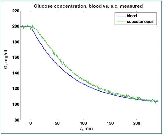
Simulated change in capillary blood glucose (G) and the corresponding interstitial fluid sensor signal. A lag of 12 minutes between capillary blood and interstitial fluid is assumed, and sensor noise with a standard deviation of 1 mg/dl is used. s.c., subcutaneous.

Rebrin and colleagues⁶⁵ presented an intuitive estimation approach by rearranging Equation (37) to solve for blood glucose (g) from the subcutaneous sensor signal (y):

$$\hat{g}=\frac{\frac{dy}{dt}-ay}{b},$$ (38)

where ˆ is used to indicate an estimated value. A finite-differences (FD) approximation for the derivative yields

$$\begin{array}{l}{\stackrel{\mathbf{ˆ}}{\mathit{g}}}_{\mathit{k}}\mathbf{=}\frac{\frac{{\mathit{y}}_{\mathit{k}}\mathbf{-}{\mathit{y}}_{\mathit{k}\mathbf{-}\mathbf{1}}}{\mathbf{\Delta }\mathit{t}}\mathbf{-}\mathit{a}{\mathit{y}}_{\mathit{k}}}{\mathit{b}}\\ {\stackrel{\mathbf{ˆ}}{\mathit{g}}}_{\mathit{k}}\mathbf{=}\mathbf{\left(}\frac{\mathbf{1}}{\mathit{b}\mathbf{\Delta }\mathit{t}}\mathbf{-}\frac{\mathit{a}}{\mathit{b}}\mathbf{\right)}{\mathit{y}}_{\mathit{k}}\mathbf{+}\mathbf{\left(}\mathbf{-}\frac{\mathbf{1}}{\mathit{b}\mathbf{\Delta }\mathit{t}}\mathbf{\right)}{\mathit{y}}_{\mathit{k}\mathbf{-}\mathbf{1}}\mathbf{.}\end{array}$$ (39)

Rebrin and colleagues⁶⁵ noted that this numerical derivative-based approach is very sensitive to measurement noise and also applied a three-point moving average filter to the derivative term. It should be made clear that Medtronic does not use this FD approach for lag compensation in their products; it is used here merely to show the major advantages of optimal estimation-based techniques for this type of problem. The Medtronic patent by Steil and Rebrin³⁰ cites the use of a Weiner filter for lag compensation, but no technical details are provided. The Abbott patent by Feldman and McGarraugh¹⁷ describes a lag compensation procedure identical to Equation (39), when y is a calibrated sensor value (and thus a/b = −1).

Bequette⁶⁸ developed a Kalman filter-based algorithm to compensate for the blood glucose to interstitial fluid transport lag, even when there is substantial sensor noise. A formulation that assumes that the stochastic noise term perturbs the glucose rate of change is shown in the following equation

$$\begin{array}{llll}\left[\begin{array}{c}{s}_{k+1}\\ g_{k+1}\\ d_{k+1}\end{array}\right]=\left[\begin{array}{ccc}\mathbf{\Phi }& \mathbf{\Gamma }& 0\\ 0& 1& 1\\ 0& 0& 1\end{array}\right]\left[\begin{array}{c}{s}_k\\ g_k\\ d_k\end{array}\right]+\left[\begin{array}{c}0\\ 0\\ 1\end{array}\right]w_k\hfill & \hfill & \hfill & \hfill \\ y_k=\left[\begin{array}{ccc}1& 0& 0\end{array}\right]\left[\begin{array}{c}{s}_k\\ g_k\\ d_k\end{array}\right]+{\upsilon }_k\hfill & \hfill & \hfill & ,\hfill \end{array}$$ (40)

where s is the subcutaneous glucose concentration, g is the capillary blood glucose, and d is the rate of change of blood glucose. The time lag of 12 minutes and the gain of 1 result in values of Φ = exp(−Δt/τ) = 0.92 and Γ 1 − Φ = 0.08. The state estimates are obtained solving Equations (22) and (23) as before. For these simulation studies, the steady-state Kalman gain is obtained by iterating Equations (24) and (25) until they converge to constant values.

A comparison of FD with Kalman filter estimates is shown in Figure 5, where the Kalman filter is designed based on Q = 0.005 and R = 1 and on the steady-state Kalman gain (L_ss). Clearly the Kalman filter estimates are insensitive to sensor noise, with the downside of a slight lag in the estimates when glucose begins to decrease. This lag can be reduced by using a larger Q value in the design, with a slight increase in noise sensitivity.

Figure 5.

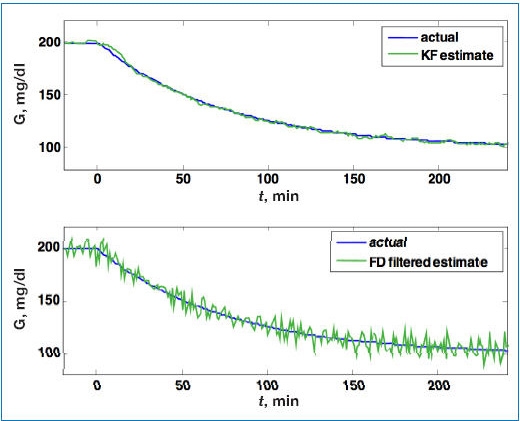
Comparison of estimated blood glucose (G) from a Kalman filter (KF; top), with the FD estimator (bottom), based on the simulated sensor signal in Figure 4. While there is a slight lag immediately after the initial decrease in blood glucose using the Kalman filter, much less noise propagates into the estimate compared to the FD approach.

Another approach that can be used to estimate capillary blood glucose from noisy subcutaneous sensor signals is Phillips–Tikhonov regularization, as shown by Freeland and Bonnecaze.⁶⁹ Essentially their method involves an analytical integration of Equation (37) to the form of

$$y\left(t\right)=y\left(\text{θ}\right)\exp \left(-\left(t-\text{θ}\right)/\tau \right)+{\displaystyle \underset{\text{θ}}{\overset{t}{\int }}\frac{g(\gamma )}{\tau }\exp \left(\left(t-\gamma \right)/\tau \right)d\text{γ,}}$$ (41)

where θ is the initial time for a window of data that includes the current time, t. Discretization and inversion methods are then used to solve for the unknown glucose as a function of time, g(t). This method appears to be more sensitive to measurement noise than Kalman filtering, however.

Discussion

There are a number of limitations to the performance of a blood glucose estimator, no matter which approach is used. One is the dynamic relationship between capillary blood glucose and the subcutaneous sensor signal, which may actually be time varying. Another limitation is the static calibration curve relating the subcutaneous signal to the capillary blood glucose; this is strongly dependent on the quality of the calibration, which is dependent on the glucose meter variability as well as the “human element.”

Signal Dropouts and Related Artifacts

A simple way to detect signal dropouts is to set a bound on allowable measurement changes. That is, a measurement is invalid if

$$\begin{array}{l}\left|y_k-y_{k-1}\right|>\text{δ}\hfill \\ y_k<\epsilon \hfill \end{array},$$ (42)

where δ is a rate-of-change threshold. Because the rate of change is sensitive to noise, consider the use of a Kalman filter, with glucose rate of change as the second state

$${\hat{x}}_{k|k}={\left[\begin{array}{c}\hat{g}\\ \hat{d}\end{array}\right]}_{k|k}.$$ (43)

If $\left|{\hat{d}}_{k|k}\right|>\delta$, then a revised glucose estimate could be ${\hat{g}}_{k|k}={\hat{g}}_{k-1|k-1}\pm \delta$. This prediction could be carried out for j time steps of an invalid signal using

$${\hat{x}}_{k+j|k}={\mathbf{\Phi }}^j{\hat{x}}_{k|k}.$$ (44)

An alarm could be activated after a certain number of steps without a valid signal or when “open-loop” covariances indicate that an individual is possibly entering an unsafe condition.

Bondia and colleagues⁷⁰ discussed the use of support vector machines to detect incorrect measurements; their method is based on retrospective analysis, but note that a real-time approach is desirable. Monitoring techniques for fault detection and abnormal situation management are often used in the chemical process industries, and it is likely that these techniques could be used successfully for CGM fault detection. For example, Juricek and associates⁷¹ presented a Kalman filter-based approach to predict whether a process variable will violate an emergency limit in the future.

It is also standard in the chemical process industries to use redundant measurements to reconcile errors and detect gross errors and failures. Ward and colleagues⁷² proposed a similar idea, but developed a sensor array with four implantable sensors. They used a median-based algorithm to detect when one of the sensor signals is inconsistent with the other sensors.

Conclusions

A concise review of many of the published algorithms proposed for CGM calibration, filtering, hypo- and hyperglycemia prediction, and fault detection has been conducted. A tutorial exposition on the use of Kalman filtering for improved glucose (and rate of change) estimation and prediction is provided. Significant progress needs to be made in sensor fault detection, as well as integration of all of the components into a robust, reliable hardware and software platform.

Abbreviations

ANN

artificial neural networks

AR

autoregressive

CGM

continuous glucose monitoring

CGMS

continuous glucose monitoring system

FD

finite differences

FDA

Food and Drug Administration

FIR

finite impulse response

FSN-CGM

FreeStyle Navigator continuous glucose monitoring

IIR

infinite impulse response

SMBG

self-monitoring blood glucose

Appendix: Simulation Parameters

A1. Linear Decrease in Glucose Example

The simulation shown in Figure 1 is based on a glucose rate of change (slope) of −2 mg/dl/min, starting at 150 mg/dl, with random sensor noise with a standard deviation of 2 mg/dl.

A2. Kalman Filter Applied to Linear Decrease in Glucose Example

Simulation details for Figures 2 and 3 are provided next. The state and measurement variances are

$$\begin{array}{ll}Q={0.1}^2\hfill & {\text{mg}}^2/{\text{dl}}^2/{\text{min}}^2\hfill \\ R=2^2\hfill & {\text{mg}}^2/{\text{dl}}^2.\hfill \end{array}$$

The following initial conditions are used for the state vector and the state covariance

$$\begin{array}{l}{P}_0=\left[\begin{array}{ll}{2}^2\hfill & 0\hfill \\ 0\hfill & 2^2\hfill \end{array}\right]\hfill \\ {\hat{x}}_0=\left[\begin{array}{l}{\hat{g}}_0\hfill \\ {\hat{d}}_0\hfill \end{array}\right]=\left[\begin{array}{l}{y}_0\hfill \\ 0\hfill \end{array}\right]=\left[\begin{array}{c}153.2\\ 0\end{array}\right].\hfill \end{array}$$

Thus there is significant initial uncertainty in the states, as the actual initial condition is

$$x_0=\left[\begin{array}{c}{g}_0\\ d_0\end{array}\right]=\left[\begin{array}{c}150\\ -2\end{array}\right].$$

The Kalman gain (L) at the end of 15 minutes of measurements is

$$L_{k=15}=\left[\begin{array}{l}0.5371\hfill \\ 0.0436\hfill \end{array}\right],$$

which eventually converges to the steady-state Kalman gain of

$$L_{\text{ss}}=\left[\begin{array}{l}0.2716\hfill \\ 0.0427\hfill \end{array}\right].$$

The state covariance matrix of

$$P_{k=15}=\left[\begin{array}{ll}4.6415\hfill & 0.3770\hfill \\ 0.3770\hfill & 0.1025\hfill \end{array}\right]$$

eventually converges to a steady-state value of

$$P_{\text{ss}}=\left[\begin{array}{ll}1.4914\hfill & 0.2343\hfill \\ 0.2343\hfill & 0.0736\hfill \end{array}\right].$$

That is, eventually (with continued measurement updates), variances of the glucose and rate-of-changes estimates are 1.49 and 0.0736 mg²/dl²/min², respectively, yielding long-term confidence intervals of ±1.22 mg/dl and ±0.27 mg/dl/min for glucose and its rate of change.

A3. Estimation of Capillary Blood Glucose from Noisy Subcutaneous Sensor Example

Simulation details for Figures 4 and 5 are presented here. The process covariance, Q = 0.005, and the sensor noise, R = 1 (consistent with the measurement noise variance of 1 mg²/dl²). The steady-state Kalman gain is

$$L_{\text{ss}}=\left[\begin{array}{l}0.2522\hfill \\ 0.7221\hfill \\ 0.0611\hfill \end{array}\right]$$

and the steady-state state covariance matrix is

$$P_{\text{ss}}=\left[\begin{array}{lll}0.3373\hfill & 0.9656\hfill & 0.0818\hfill \\ 0.9656\hfill & 3.4424\hfill & 0.3781\hfill \\ 0.0818\hfill & 0.3781\hfill & 0.064\hfill \end{array}\right].$$

That is, the steady-state variance of the estimate of subcutaneous glucose (measured) is 0.3373 mg²/dl², capillary blood glucose (unmeasured) is 3.4424 mg²/dl², and the rate of change of blood glucose (unmeasured) is 0.064 mg²/dl²/min².

References

- 1.Bequette BW. A critical assessment of algorithms and challenges in the development of an artificial pancreas. Diabetes Technol Ther. 2005;7(1):28–47. doi: 10.1089/dia.2005.7.28. [DOI] [PubMed] [Google Scholar]
- 2.Doyle FJ, 3rd, Jovanovic L, Seborg DE. A tutorial on biomedical process control: glucose control strategies for treating type 1 diabetes mellitus. J Process Control. 2007;17(7):572–576. [Google Scholar]
- 3.Kumareswaran K, Evans ML, Hovorka R. Artificial pancreas: an emerging approach to treat type 1 diabetes. Expert Rev Med Dev. 2009;6(4):401–410. doi: 10.1586/erd.09.23. [DOI] [PubMed] [Google Scholar]
- 4.Cobelli C, Dalla Man C, Sparacino G, Magni L, De Nicolao G, Kovatchev B. Diabetes: models, signals and control. IEEE Rev Biomed Eng. 2010:3. doi: 10.1109/RBME.2009.2036073. In press. [DOI] [PMC free article] [PubMed] [Google Scholar]
- 5.Klonoff DC. Continuous glucose monitoring: roadmap for 21st century diabetes therapy. Diabetes Care. 2005;28(5):1231–1239. doi: 10.2337/diacare.28.5.1231. [DOI] [PubMed] [Google Scholar]
- 6.Klonoff DC. A review of continuous glucose monitoring technology. Diabetes Technol Ther. 2005;7(5):770–775. doi: 10.1089/dia.2005.7.770. [DOI] [PubMed] [Google Scholar]
- 7.JDRF CGM Study Group. JDRF randomized clinical trial to assess the efficacy of real-time continuous glucose monitoring in the management of type 1 diabetes: research design and methods. Diabetes Technol Ther. 2008;10(4):310–321. doi: 10.1089/dia.2007.0302. [DOI] [PubMed] [Google Scholar]
- 8.Skyler JS. Continuous glucose monitoring: an overview of its development. Diabetes Technol Ther. 2009;1(11 Suppl):S5–S10. doi: 10.1089/dia.2009.0045. [DOI] [PubMed] [Google Scholar]
- 9.Kerr D, Fayers K. Continuous real-time glucose monitoring systems: time for a closer look. Pract Diab Int. 2008;25(1):37–41. [Google Scholar]
- 10.Oliver NS, Toumazou C, Cass AE, Johnston DG. Glucose sensors: a review of current and emerging technology. Diab Med. 2009;26(3):197–210. doi: 10.1111/j.1464-5491.2008.02642.x. [DOI] [PubMed] [Google Scholar]
- 11.Cox M. An overview of continuous glucose monitoring systems. J Pediatr Health Care. 2009;23(5):344–347. doi: 10.1016/j.pedhc.2009.06.002. [DOI] [PubMed] [Google Scholar]
- 12.Klonoff D, Bernhardt P, Ginsberg BH, Joseph J, Mastrototaro J, Parker DR, Vesper H, Vigersky R. CLSI document POCT05-A (ISBN 1-56238-685-9) Clinical and Laboratory Standards Institute; 2008. Performance metrics for continuous interstitial glucose monitoring; approved guideline. [Google Scholar]
- 13.Lodwig V, Heinemann L. Continuous glucose monitoring with glucose sensors: calibration and assessment criteria. Diabetes Technol Ther. 2003;5(4):573–587. doi: 10.1089/152091503322250596. [DOI] [PubMed] [Google Scholar]
- 14.Hayter PG, Sharma M, Dunka L, Stout P, Price DA, Horwitz DL, Marhoul J, Vaez-Zadeh S. Performance standards for continuous glucose monitors. Diabetes Technol Ther. 2005;7(5):721–726. doi: 10.1089/dia.2005.7.721. [DOI] [PubMed] [Google Scholar]
- 15.Shiavi R. 3rd ed. Academic Press; 2007. Introduction to applied statistical signal analysis. [Google Scholar]
- 16.Goode PV, Jr, Brauker JH, Kamath AU. System and methods for processing analyte sensor data. United States patent US 6,931,327 B2. 2005 Aug 16; [Google Scholar]
- 17.Feldman BJ, McGarraugh GV. Method of calibrating an analyte-measurement device, and associated methods, devices and systems. United States patent US 7,299,082 B2. 2007 Nov 20; [Google Scholar]
- 18.Ginsberg BH. Factors affecting blood glucose monitoring: sources of errors in measurement. J Diabetes Sci Technol. 2009;3(4):903–913. doi: 10.1177/193229680900300438. [DOI] [PMC free article] [PubMed] [Google Scholar]
- 19.Panteleon A, Rebrin K, Steil GM. The role of the independent variable to glucose sensor calibration. Diabetes Technol Ther. 2003;5(3):401–410. doi: 10.1089/152091503765691901. [DOI] [PubMed] [Google Scholar]
- 20.Choleau C, Klein JC, Reach G, Aussedat B, Demaria-Pesce V, Wilson GS, Gifford R, Ward WK. Calibration of a subcutaneous amperometric glucose sensor. Part 1. Effect of measurement uncertainties on the determination of sensor sensitivity and background current. Biosens Bioelectron. 2002;17(8):641–646. doi: 10.1016/s0956-5663(01)00306-2. [DOI] [PubMed] [Google Scholar]
- 21.Choleau C, Klein JC, Reach G, Aussedat B, Demaria-Pesce V, Wilson GS, Gifford R, Ward WK. Calibration of a subcutaneous amperometric glucose sensor implanted for 7 days in diabetic patients. Part 2. Superiority of the one-point calibration method. Biosens Bioelectron. 2002;17(8):647–654. doi: 10.1016/s0956-5663(01)00304-9. [DOI] [PubMed] [Google Scholar]
- 22.Clark WL, Cox D, Gonder-Frederick LA, Carter W, Pohl SL. Evaluating clinical accuracy of systems for self-monitoring of blood glucose. Diabetes Care. 1987;10(5):622–628. doi: 10.2337/diacare.10.5.622. [DOI] [PubMed] [Google Scholar]
- 23.Aussedat B, Thome´-Duret V, Reach G, Lemmonier F, Klein JC, Hu Y, Wilson GS. A user-friendly method for calibrating a subcutaneous glucose sensor-based hypoglycaemic alarm. Biosens Bioelectron. 1997;12(11):1061–1071. doi: 10.1016/s0956-5663(97)00083-3. [DOI] [PubMed] [Google Scholar]
- 24.King C, Anderson SM, Breton M, Clarke WJ, Kovatchev B. Modeling of calibration effectiveness and blood-to-interstitial glucose dynamics as potential confounders of the accuracy of continuous glucose sensors during hyperinsulinemic clamp. J Diabetes Sci Technol. 2007;1(3):317–322. doi: 10.1901/jaba.2007.1-317. [DOI] [PMC free article] [PubMed] [Google Scholar]
- 25.DirectNet Study Group. Evaluation of factors affecting CGMS calibration. Diabetes Technol Ther. 2006;8(1):318–325. doi: 10.1089/dia.2006.8.318. [DOI] [PMC free article] [PubMed] [Google Scholar]
- 26.Poitout V, Moatti-Sirat D, Reach G, Zhang Y, Wilson GS, Lemonnier F, Klein JC. A glucose monitoring system for on line estimation in man of blood glucose concentration using a miniaturized glucose sensor implanted in the subcutaneous tissue and a wearable control unit. Diabetologia. 1993;36(7):658–663. doi: 10.1007/BF00404077. [DOI] [PubMed] [Google Scholar]
- 27.Mastrototaro JJ, Gross TM, Shin JJ. Glucose monitor calibration methods. United States patent US 6,424,847. 2002 Jul 23; [Google Scholar]
- 28.Shin JJ, Holtzclaw KR, Dangui ND, Kanderian S, Jr, Mastrototaro JJ, Hong PI. Real time self-adjusting calibration algorithm. United States patent US 6,895,263 B2. 2005 May 17; [Google Scholar]
- 29.Keenan DB, Mastrototaro JJ, Voskanyan G, Steil GM. Delays in minimally invasive continuous glucose monitoring devices: a review of current technology. J Diabetes Sci Technol. 2009;3(5):1207–1214. doi: 10.1177/193229680900300528. [DOI] [PMC free article] [PubMed] [Google Scholar]
- 30.Steil G, Rebrin K. Closed-loop system for controlling insulin infusion. United States patent US 7,354,420 B2. 2008 Apr 8; [Google Scholar]
- 31.Knobbe EJ, Buckingham B. The extended Kalman filter for continuous glucose monitoring. Diabetes Technol Ther. 2005;7(1):15–27. doi: 10.1089/dia.2005.7.15. [DOI] [PubMed] [Google Scholar]
- 32.Knobbe EJ, Lim WL, Buckingham BA. Method and apparatus for real-time estimation of physiological parameters. United States patent US 6,575,905 B2. 2003 Jun 10; [Google Scholar]
- 33.Bequette BW, Palerm CC, Willis JP, Desemone J. Incorporation of glucose meter uncertainty in the calibration of continuous glucose sensors. Diabetes Technol Ther. 2005;7(2):366–367. [Google Scholar]
- 34.Kuure-Kinsey M, Palerm CC, Bequette BW. A dual-rate Kalman filter for continuous glucose monitoring. Proc. IEEE EMB Conference; 2006. pp. 63–66. [DOI] [PubMed] [Google Scholar]
- 35.Heise T, Koschinsky T, Heinemann L, Lodwig V. Hypoglycemia warning signal and glucose sensors: requirements and concepts. Diabetes Technol Ther. 2003;5:563–571. doi: 10.1089/152091503322250587. [DOI] [PubMed] [Google Scholar]
- 36.Buckingham B. Clinical overview of continuous glucose monitoring. J Diabetes Sci Technol. 2008;2(2):300–306. doi: 10.1177/193229680800200223. [DOI] [PMC free article] [PubMed] [Google Scholar]
- 37.Noujaim SE, Horwitz D, Sharma M, Marhoul J. Accuracy requirements for a hypoglycemia detector: an analytical model to evaluate the effects of bias, precision, and the rate of glucose change. J Diabetes Sci Technol. 2007;1(5):652–668. doi: 10.1177/193229680700100509. [DOI] [PMC free article] [PubMed] [Google Scholar]
- 38.Brauker J. Continuous glucose sensing: future technology developments. Diabetes Technol Ther. 2009;1(11 Suppl):S25–S36. doi: 10.1089/dia.2008.0137. [DOI] [PubMed] [Google Scholar]
- 39.McGarraugh G, Bergenstal R. Detection of hypoglycemia with continuous interstitial and traditional blood glucose monitoring using the Freestyle Navigator continuous glucose monitoring system. Diabetes Technol Ther. 2009;11(3):145–150. doi: 10.1089/dia.2008.0047. [DOI] [PubMed] [Google Scholar]
- 40.Cameron FM, Niemeyer G, Palerm CC, Dassau E, Doyle FJ, 3rd, Lee H, Bequette BW, Chase HP, Buckingham BA. Early detection of hypoglycemia combining multiple predictive methods on retrospective clinical continuous glucose monitoring data. J Diabetes Sci Technol. 2008;2(2):A19. [Google Scholar]
- 41.Dassau E, Cameron FM, Lee H, Bequette BW, Doyle FJ, 3rd, Niemeyer G, Chase P, Buckingham BA. Real-time hypoglycemia prediction using continuous glucose monitoring (CGM), a safety net to the artificial pancreas. Diabetes. 2008;57(Suppl):A13. doi: 10.2337/dc09-1487. [DOI] [PMC free article] [PubMed] [Google Scholar]
- 42.Buckingham B, Cobry E, Clinton P, Gage V, Caswell K, Kunselman E, Cameron F, Chase HP. Preventing hypoglycemia using predictive alarm algorithms and insulin pump suspension. Diabetes Technol Ther. 2009;11(2):93–97. doi: 10.1089/dia.2008.0032. [DOI] [PMC free article] [PubMed] [Google Scholar]
- 43.Choleau C, Dokladal P, Klein JC, Ward WK, Wilson GS, Reach G. Prevention of hypoglycemia using risk assessment with a continuous glucose monitoring system. Diabetes Care. 2002;51(11):3263–3273. doi: 10.2337/diabetes.51.11.3263. [DOI] [PubMed] [Google Scholar]
- 44.Cameron F, Niemayer G, Gundy-Burlet K, Buckingham B. Statistical hypoglycemia prediction. J Diabetes Sci Technol. 2008;2(4):612–621. doi: 10.1177/193229680800200412. [DOI] [PMC free article] [PubMed] [Google Scholar]
- 45.Dunn TC, Jayalakshmi Y, Kurnik RT, Lesho MJ, Oliver JJ, Potts RO, Tamada JA, Waterhouse SR, Wei CW. Method and device for predicting physiological values. United States patent US 6,653,091 B1. 2003 Nov 25; [Google Scholar]
- 46.Palerm CC, Willis JP, Desemone J, Bequette BW. Hypoglycemia prediction and detection using optimal estimation. Diabetes Technol Ther. 2005;7(1):3–14. doi: 10.1089/dia.2005.7.3. [DOI] [PubMed] [Google Scholar]
- 47.Palerm CC, Bequette BW. Hypoglycemia detection and prediction using continuous glucose monitoring–a study on hypoglycemic clamp data. J Diabetes Sci Technol. 2007;1(5):624–629. doi: 10.1177/193229680700100505. [DOI] [PMC free article] [PubMed] [Google Scholar]
- 48.Stengel RF. New York: Dover; 1994. Optimal control and estimation. [Google Scholar]
- 49.Facchinetti A, Sparacino G, Cobelli C. IEEE Trans Biomed Eng. 2010. An on-line self-tuneable method to denoise CGM sensor data; p. 57. In press. [DOI] [PubMed] [Google Scholar]
- 50.Bremer T, Gough DA. Is blood glucose predictable from previous values? A solicitation for data. Diabetes. 1999;48(3):445–451. doi: 10.2337/diabetes.48.3.445. [DOI] [PubMed] [Google Scholar]
- 51.Reifman J, Rajaraman S, Gribok A, Ward WK. Predictive monitoring for improved management of glucose levels. J Diabetes Sci Technol. 2007;1(4):478–486. doi: 10.1177/193229680700100405. [DOI] [PMC free article] [PubMed] [Google Scholar]
- 52.Gani A, Gribok AV, Rajaraman S, Ward WK, Reifman J. Predicting subcutaneous glucose concentration in humans: data-driven glucose modeling. IEEE Trans Biomed Eng. 2009;56(2):246–254. doi: 10.1109/TBME.2008.2005937. [DOI] [PubMed] [Google Scholar]
- 53.Sparacino G, Zanderigo F, Corazza S, Maran A, Facchinetti A, Cobelli C. Glucose concentration can be predicted ahead in time from continuous glucose monitoring sensor time series. IEEE Trans Biomed Eng. 2007;54(5):931–937. doi: 10.1109/TBME.2006.889774. [DOI] [PubMed] [Google Scholar]
- 54.Zanderigo F, Sparacino G, Kovatchev BP, Cobelli C. Glucose prediction algorithms from continuous monitoring data: assessment of accuracy via continuous glucose-error grid analysis. J Diabetes Sci Technol. 2007;1(5):645–651. doi: 10.1901/jaba.2007.1-645. [DOI] [PMC free article] [PubMed] [Google Scholar]
- 55.Sparacino G, Facchinetti A, Maran A, Cobelli Continuous glucose monitoring time series and hypo/hyperglycemia prevention: requirements, methods, open problems. Curr Diabetes Rev. 2008;4(3):181–192. doi: 10.2174/157339908785294361. [DOI] [PubMed] [Google Scholar]
- 56.Gani A, Gribok AV, Lu Y, Ward WK, Vigersky RA, Reifman J. Universal glucose models for predicting subcutaneous glucose concentration in humans. IEEE Trans Inf Tech Biomed. 2010;14(1):157–165. doi: 10.1109/TITB.2009.2034141. [DOI] [PubMed] [Google Scholar]
- 57.Eren-Oruklu M, Cinar A, Quinn L, Smith D. Estimation of future glucose concentrations with subject-specific recursive linear models. Diabetes Technol Ther. 2009;11(4):243–253. doi: 10.1089/dia.2008.0065. [DOI] [PMC free article] [PubMed] [Google Scholar]
- 58.Eren-Oruklu M, Cinar A, Quinn L. Hypoglycemia prediction with subject-specific recursive time-series models. J Diabetes Sci Technol. 2010;4(1):25–33. doi: 10.1177/193229681000400104. [DOI] [PMC free article] [PubMed] [Google Scholar]
- 59.Pappada SM, Camero BD, Rosman PM. Development of a neural network for prediction of glucose concentration in type 1 diabetes patients. J Diabetes Sci Technol. 2008;2(5):792–801. doi: 10.1177/193229680800200507. [DOI] [PMC free article] [PubMed] [Google Scholar]
- 60.Kuure-Kinsey M, Cutright R, Bequette BW. Computationally efficient neural predictive control based on a feedforward architecture. Ind Eng Chem Res. 2006;45(25):8575–8582. [Google Scholar]
- 61.Kuure-Kinsey M, Bequette BW. Improved nonlinear predictive control performance using recurrent neural networks. Proceedings of the 2008 American Control Conference; Seattle, Washington. pp. 4197–4202. [Google Scholar]
- 62.Weinstein RL, Schwartz S, Brazg RL, Bugler JR, Peyser TA, McGarraugh GV. Accuracy of the 5-day FreeStyle Navigator continuous glucose monitoring system. Diabetes Care. 2007;30(3):1125–1130. doi: 10.2337/dc06-1602. [DOI] [PubMed] [Google Scholar]
- 63.Voskanyan G, Keenan DB, Mastrototaro JJ, Steil GM. Putative delays in interstitial fluid (ISF) glucose kinetics can be attributed to the glucose sensing systems used to measure them rather than the delay in ISF glucose itself. J Diabetes Sci Technol. 2007;1(5):639–644. doi: 10.1177/193229680700100507. [DOI] [PMC free article] [PubMed] [Google Scholar]
- 64.Schmidtke DW, Freeland AC, Heller A, Bonnecaze R. Measurement and modeling of the transient difference between blood and subcutaneous glucose concentrations in the rat after injection of insulin. Proc Natl Acad Sci U S A. 1998;95(1):294–299. doi: 10.1073/pnas.95.1.294. [DOI] [PMC free article] [PubMed] [Google Scholar]
- 65.Rebrin K, Steil GM, Van Antwerp WP, Mastrototaro JJ. Subcutaneous glucose predicts plasma glucose independent of insulimplications for continuous monitoring. Am J Physiol. 1999;277(3 Pt 1):E561–E571. doi: 10.1152/ajpendo.1999.277.3.E561. [DOI] [PubMed] [Google Scholar]
- 66.Steil GM, Rebrin K, Mastrototaro J, Bernaba B, Saad MF. Determination of plasma glucose during rapid glucose excursions with a subcutaneous glucose sensor. Diabetes Technol Ther. 2003;5(1):27–31. doi: 10.1089/152091503763816436. [DOI] [PubMed] [Google Scholar]
- 67.Kulcu E, Tamada JA, Reach G, Potts RO, Lesho MJ. Physiological differences between interstitial glucose and blood glucose measured in human subjects. Diabetes Care. 2003;26(8):2405–2409. doi: 10.2337/diacare.26.8.2405. [DOI] [PubMed] [Google Scholar]
- 68.Bequette BW. Optimal estimation applications to continuous glucose monitoring. Proceedings of the 2004 American Control Conference; 2004. pp. 958–962. [Google Scholar]
- 69.Freeland AC, Bonnecaze RT. Inference of blood glucose concentrations from subcutaneous glucose concentrations: applications to glucose biosensors. Ann Biomed Eng. 1999;27(4):525–537. doi: 10.1114/1.196. [DOI] [PubMed] [Google Scholar]
- 70.Bondia J, Tarin C, Garcia-Gabin W, Esteve E, Fernandez-Real JM, Ricart W, Vehi J. Using support vector machines to detect therapeutically incorrect measurements by the MiniMed CGMS. J Diabetes Sci Technol. 2008;2(4):622–629. doi: 10.1177/193229680800200413. [DOI] [PMC free article] [PubMed] [Google Scholar]
- 71.Juricek BC, Seborg DE, Larimore WE. Predictive monitoring for abnormal situation management. J Process Control. 2001;11:111–128. [Google Scholar]
- 72.Ward WK, Casey HM, Quinn MJ, Federiuk IF, Wood MD. A fully implantable subcutaneous glucose sensor array: enhanced accuracy from multiple sensing units and a median-based algorithm. Diabetes Technol Ther. 2003;5(6):943–952. doi: 10.1089/152091503322640980. [DOI] [PubMed] [Google Scholar]